PHYSICS of TRANSPORT and TRAFFIC PHENOMENA in BIOLOGY:
from molecular motors and cells to organisms

Abstract

Traffic-like collective movements are observed at almost all levels of biological systems. Molecular motor proteins like, for example, kinesin and dynein, which are the vehicles of almost all intra-cellular transport in eukayotic cells, sometimes encounter traffic jam that manifests as a disease of the organism. Similarly, traffic jam of collagenase MMP-1, which moves on the collagen fibrils of the extracellular matrix of vertebrates, has also been observed in recent experiments. Novel efforts have been made to utilize some uni-cellular organisms as “micro-transporters”. Traffic-like movements of social insects like ants and termites on trails are, perhaps, more familiar in our everyday life. Experimental, theoretical and computational investigations in the last few years have led to a deeper understanding of the generic or common physical principles involved in these phenomena. In this review we critically examine the current status of our understanding, expose the limitations of the existing methods, mention open challenging questions and speculate on the possible future directions of research in this interdisciplinary area where physics meets not only chemistry and biology but also (nano-)technology.

I Introduction

Motility is the hallmark of life. From intracellular molecular transport and crawling of amoebae to the swimming of fish and flight of birds, movement is one of life’s central attributes. All these ”motile” elements generate the forces required for their movements by actively converting some other forms of energy into mechanical energy. However, in this review we are interested in a special type of collective movement of these motile elements. What distinguishes a traffic-like movement from all other forms of movements is that traffic flow takes place on “tracks” and “trails” (like those for trains and street cars or like roads and highways for motor vehicles) for the movement of the motile elements. From now onwards, the term “element” will mean the motile element under consideration.

We are mainly interested in the general principles and common trends seen in the mathematical modeling of collective traffic-like movements at different levels of biological organization. We begin at the lowest level, starting with intracellular biomolecular motor traffic on filamentary rails and end our review by discussing the collective movements of social insects (like, for example, ants and termites) and vertebrates on trails. Some examples of motile elements and the corresponding tracks are shown in fig.1.

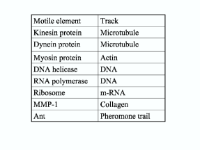
Figure 1: Examples of motile elements and the corresponding tracks.

I.1 Different types of traffic in biology

Now we shall give a few examples of the traffic-like collective phenomena in biology to emphasize some dynamical features of the tracks which makes biological traffic phenomena more exotic as compared to vehicular traffic. In any modern society, the most common traffic phenomenon is that of vehicular traffic. The changes in the roads and highway networks take place over periods of years (depending on the availability of funds) whereas a vehicle takes a maximum of a few hours for a single journey. Therefore, for all practical purposes, the roads can be taken to be independent of time while studying the flow of vehicular traffic. In sharp contrast, the tracks and trails, which are the biological analogs of roads, can have nontrivial dependence on time during the typical travel time of the motile elements. We give a few examples of such traffic.

$\bullet$ Time-dependent track whose length and shape can be affected by the motile element: Microtubules, a class of filamentary proteins, serve as tracks for two superfamilies of motor proteins called kinesins and dyneins howard ; schliwa ; hackney . Interestingly, microtubules are known to exhibit an unusual polymerization-depolymerization dynamics even in the absence of motor proteins. Moreover, in some circumstances, the motor proteins interact with the microtubule tracks so as to influence their length as well as shape; one such situation arises during cell division (the process is called mitosis).

$\bullet$ Time-dependent track/trail created and maintained by the motile element: A DNA helicase patel ; crampton unwinds a double-stranded DNA and uses one of the single strands thus opened as the track for its own translocation. Ants are known to create the trails by dropping a chemical which is generically called pheromone wilson . Since the pheromone gradually evaporates, the ants keep reinforcing the trail in order to maintain the trail networks.

$\bullet$ Time-dependent track destroyed by the motile element: A class of enzymes, called MMP-1, degrades their tracks formed by collagen fibrils nagase ; whittaker .

Our aim is to present a critical overview of the common trends in the mathematical modelling of these traffic-like phenomena. Although the choice of the physical examples and modelling strategies are biased by our own works and experiences, we put these in a broader perspective by relating these with works of other research groups.

This review is organized as follows: the general physical principles and the methods of modelling traffic-like collective phenomena are discussed in sections II-VI while specific examples are presented in the remaining sections. A summary of the various theoretical approaches followed so far in given in section II. The totally asymmetric simple exclusion process (TASEP), which lies at the foundation of the theoretical formalism that we have used successfully in most of our own works so far, has been described separately in section III. The Brownian ratchet mechanism, an idealized generic mechanism of directed, albeit noisy, movement of single molecular motors, is explained in section IV. Traffic of ribosomes, a class of nucleotide-based motors, is considered in section V. Intracellular traffic of cytoskeletal motors is discussed in detail in section VI while those of matrix metalloproteases in the extra-cellular matrix is summarized in section VII. Models of traffic of cells, ants and humans on trails are sketched in sections VIII, IX and X. The main conclusions regarding the common trends of modelling the traffic-like collective phenomena in diverse systems over a wide range of length scales are summarized in section XI.

II Different types of theoretical approaches

First of all, the theoretical approaches can be broadly divided into two categories: (I) “Individual-based” and (II) “Population-based”. The individual-based models describe the dynamics of the individual elements explicitly. Just as “microscopic” models of matter are formulated in terms of molecular constituents, the individual-based models of transport are also developed in terms of the constituent elements. Therefore, the individual-based models are often referred to as “microscopic” models. In contrast, in the population-based models individual elements do not appear explicitly and, instead, one considers only the population densities (i.e., number of individual elements per unit area or per unit volume). The spatio-temporal organization of the elements are emergent collective properties that are determined by the responses of the individuals to their local environments and the local interactions among the individual elements. Therefore, in order to gain a deep understanding of the collective phenomena, it is essential to investigate the linkages between these two levels of biological organization.

Usually, but not necessarily, space and time are treated as continua in the population-based models and partial differential equations (PDEs) or integro-differential equations are written down for the time-dependent local collective densities of the elements. The individual-based models have been formulated following both continuum and discrete approaches. In the continuum formulation of the Lagrangian models, differential equations describe the individual trajectories of the elements.

II.1 Population-based approaches

Suppose $\rho(\vec{x},t)$ is the local density of the population of the motile elements at the coarse-grained location $\vec{x}$ at time $t$. If the elements are conserved, one can write down an equation of continuity for $\rho(\vec{x},t)$:

$$\frac{\partial\rho}{\partial t}+\vec{\nabla}\cdot\vec{J}=0.$$ (1)

where $\vec{J}$ is the current density corresponding to the population density $\rho$. In addition, depending on the nature of the motile elements and their environment, it may be possible to write an analogue of the Navier-Stokes equation for the local dynamical variable $\vec{v}(\vec{x},t)$. However, in this review we shall focus almost exclusively on works carried out following individual-based approaches.

II.2 Individual-based approaches

For developing an individual-based model, one must first specify the state of each individual element. The dynamical laws governing the time-evolution of the system must predict the state of the system at a time $t+\Delta t$, given the corresponding state at time $t$. The change of state should reflect the response of the system in terms of movement of the individual elements.

$\bullet$ Langevin equation:

One possible framework for the mathematical formulation of such models is the deterministic Newton’s equations for individual elements; each element is modelled as a “particle” subjected to some “effective forces” arising out of its interaction with the other elements. In addition, the elements may also experience viscous drag and some random forces (“noise”) that may be caused by the surrounding medium. In that case, instead of the Newton’s equation, one can use a Langevin equation coffey . In case the element is an organism that can think and take decision, capturing inter-element interaction via effective forces becomes a difficult problem.

For a particle of mass $M$ and instantaneous velocity $v$, the Langevin equation describing its motion in one-dimensional space is written as

$$M\frac{dv}{dt}=F_{\text{ext}}-\Gamma v+F_{br}(t)$$ (2)

where $F_{\text{ext}}$ is the external force acting on the particle, and $F_{br}(t)$ is the random force (noise) while the second term on the right hand side represents the viscous drag on the particle. In order that the average velocity satisfies the Newton equation for a particle in a viscous medium, we further assume that

$$\langle\xi(t)\rangle=0.$$ (3)

and

$$\langle\xi(t)\xi(t^{\prime})\rangle=2DT\delta(t-t^{\prime})$$ (4)

where, $\xi=F_{br}/M$ and, at this level of description, $D$ is a phenomenological parameter. The prefactor $2$ on the right hand side of equation (4) has been chosen for convenience.

An alternative, but equivalent approach is to write down what is now generally referred to as a Fokker-Planck equation risken . In this approach, one deals with a deterministic partial differential equation for a probability density. For example, suppose $P(\vec{r},\vec{v};t|\vec{r}_{0},\vec{v}_{0})$ be the conditional probability that, at time $t$, the motile element is located at $\vec{r}$ and has velocity $\vec{v}$, given that its initial (i.e., at time $t=0$) position and velocity were $\vec{r}_{0},\vec{v}_{0}$. Since the total probability integrated over all space and all velocities is conserved (i.e,, does not change with time), the probability density $P$ satisfies an equation of continuity. The probability current density gets contribution not only from a diffusive motion of the motile elements but also a drift caused by the external force.

Often it turns out that real forces (i.e., forces arising from real physical interactions) alone cannot account for the observed dynamics of the motile elements; in such situations, “social forces” have been incorporated in the equation of motion mogil3 ; gueron2 . However, a priori justification of the forms of such social forces is extremely difficult. It is also worth pointing out that, in contrast to passive Brownian particles, the motile agents are active Brownian particles schweitzer .

$\bullet$ Hybrid approaches:

Suppose a set of “particles”, each of which represents a motile element, move in a potential field $U[\sigma(x)]$, where the potential at any arbitrary location $x$ is determined by the local density $\sigma(x)$ of the molecules of a chemical used by the elements for communication among themselves. In the case of ants, for example, such chemicals are generically called “pheromone”. Consequently, each “particle” experiences an “inertial”force $\vec{F}(x)=-\nabla U(x)$. Each “particle” is also assumed to be subjected to a “frictional force” where “friction” merely parametrizes the tendency of an element to continue in a given direction: a smaller “friction” implies that the element’s velocity persists for a longer time in a given direction. The motion for the “particles” is assumed to be governed by the Langevin equation

$$\ddot{x}=-\gamma{\dot{x}}-\nabla U[\sigma(x)]+\eta(t)$$ (5)

where $\eta(t)$ is a Gaussian white noise with the statistical properties

$$\langle\eta(t)\rangle=0$$ (6)

and

$$\langle\eta(t)\eta(t^{\prime})\rangle=\frac{1}{\beta}\delta(t-t^{\prime})$$ (7)

The strength $1/\beta$ of the noise determines the degree of determinacy with which the particle would follow the gradient of the local potential; the larger the value of $\beta$ the stronger is the tendency of the particle to follow the potential gradient.

Thus, the movement of an element may be described as the noisy motion of a particle in an “energy landscape”. However, this energy landscape is not static but evolves in response to the motion of the particle as each particle drops a chemical signal (pheromone) at its own location at a rate $g$ per unit time. Assuming that pheromone can diffuse in space with a diffusion constant $D$ and evaporate at a rate $\kappa$, the equation governing the pheromone field, in one-dimension, is given by

$$\frac{\partial\sigma(x,t)}{\partial t}=D\frac{\partial^{2}\sigma(x,t)}{\partial x^{2}}+g\rho(x)-\kappa\sigma(x,t)$$ (8)

where $\rho(x)$ is the local density of the particles at $x$. In order to proceed further, one has to assume a specific form of the function $U[\sigma(x)]$; one possible form assumed in the case of ants rauch is

$$U[\sigma(x)]=-\ln\biggl{(}1+\frac{\sigma}{1+\delta\sigma}\biggr{)}$$ (9)

where $1/\delta$ is called the capacity.

$\bullet$ Stochastic cellular automata:

Numerical solution of the Newton-like or Langevin-like equations require discretization of both space and time. Therefore, the alternative discrete formulations may be used from the beginning. In recent years many individual-based models, however, have been formulated on discretized space and the temporal evolution of the system in discrete time steps are prescribed as dynamical update rules using the language of cellular automata (CA) wolfram ; chopard or lattice gas (LG) marro . Since each of the individual elements may be regarded as an agent, the CA and LG models are someties also referred to as agent-based models pnas . There are some further advantages in modeling biological systems with CA and LG. Biologically, it is quite realistic to think in terms of the way each individual motile element responds to its local environment and the series of actions they perform. The lack of detailed knowledge of these behavioral responses is compensated by the rules of CA. Usually, it is much easier to devise a reasonable set of logic-based rules, instead of cooking up some effective force for dynamical equations, to capture the behaviour of the elements. Moreover, because of the high speed of simulations of CA and LG, a wide range of possibilities can be explored which would be impossible with more traditional methods based on differential equations. Most of the models we review in this article are based on CA and LG; this modelling strategy focusses mostly on generic features of the system. The average number of motile elements that arrive at (or depart from) a fixed detector site on the track per unit time interval is called the flux. One of the most important transport properties is the relation between the flux and the density of the motile elements; a graphical representation of this relation is usually referred to as the fundamental diagram. If the motile elements interact mutually only via their steric repulsion their average speed $v$ would decrease with increasing density because of the hindrance caused by each on the following elements. On the other hand, for a given density $c$, the flux $J$ is given by $J=cv(c)$, where $v(c)$ is the corresponding average speed. At sufficiently low density, the motile elements are well separated from each other and, consequently, $v(c)$ is practically independent of $c$. Therefore, $J$ is approximately proportional to $c$ if $c$ is very small. However, at higher densities the increase of $J$ with $c$ becomes slower. At high densitits, the sharp decrease of $v$ with $c$ leads to a decrease, rather than increase, of $J$ with increasing $c$. Naturally, the fundamental diagram of such a system is expected to exhibit a maxium at an intermediate value of the density.

III Asymmetric simple exclusion processes

The asymmetric simple exclusion process (ASEP) gunterrev is a simple particle-hopping model. In the ASEP particles can hop (with some probability or rate) from one lattice site to a neighbouring one, but only if the target site is not already occupied by another particle. “Simple Exclusion” thus refers to the absence of multiply occupied sites. Generically, it is assumed that the motion is “asymmetric” such that the particles have a preferred direction of motion.

For a full definition of a model, it is necessary to specify the order in which the local rule described above is to be applied to the sites. The most common update types are random-sequential dynamics and parallel dynamics. In the random-sequential case, sites are chosen in random order and then updated. In contrast, updating for the parallel case is done in a synchronous manner; here all the sites are updated at once.

Most often the one-dimensional case is studied, where particles move along a linear chain of $L$ sites. This is rather natural for many applications, e.g. for modelling highway traffic css ; mahnke . If motion is allowed in only one direction (e.g. ”to the right”), the corresponding model is sometimes called Totally Asymmetric Simple Exclusion Process (TASEP). The probability of motion from site $j$ to site $j+1$ will be denoted by $p$; in the simplest case, where all the sites are treated on equal footing, $p$ is assumed to be independent of the position of the particle.

For such driven diffusive systems the boundary conditions turn out to be crucial. If periodic boundary conditions are imposed, i.e., the sites $1$ and $L$ are made nearest-neibours of each other, all the sites are treated on the same footing. For this system the fundamental diagram has been derived exactly both in the cases of parallel and random-sequential updating rules css ; these are shown graphically in fig.2.

Figure 2: Fundamental diagrams of the TASEP with periodic boundary conditions and (a) random-sequential updating (solid curve) (b) parallel updating (dashed curve), both for $p=0.75$.

If the boundaries are open, then a particle can enter from a reservoir and occupy the leftmost site ($j=1$), with probability $\alpha$, if this site is empty. In this system a particle that occupies the rightmost site ($j=L$) can exit with probability $\beta$.

The ASEP has been studied extensively in recent years and is now well understood (see e.g. evansAlten ; gunterrev and references therein). In fact its stationary state for different dynamics can be obtained exactly derrida93 ; schdom ; rsss ; ERS ; degier . It shows an interesting phase diagram (see Fig. 3) and is the prototype for so-called boundary-induced phase transitions krug .

  

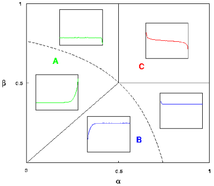
Figure 3: Processes allowed in the ASEP (left); Phase diagram of the ASEP for parallel dynamics (right) and $p=0.75$. The insets show the typical shape of the density profiles in the corresponding region. The broken line indicates points with a flat density profile.

Fig. 3 shows the generic form of the phase diagram obtained by varying the boundary rates $\alpha$ and $\beta$. One can distinguish three phases, namely (A) a low-density phase ($\alpha<\beta,\alpha_{c}(p)$), (B) a high-density phase ($\beta<\alpha,\beta_{c}(p)$) and (C) a maximal-current phase ($\alpha>\alpha_{c}(p)$ and $\beta>\beta_{c}(p)$). The appearance of these three phases can easily be understood. In the low-density phase the current depends only on the input rate $\alpha$. The input is less efficient than the transport in the bulk of the system or the output and therefore dominates the behaviour of the whole system. In the high-density phase the output is the least efficient part of the system. Therefore the current depends only on $\beta$. In the maximal current phase, input and output are more efficient than the transport in the bulk of the system. Here the current has reached the largest possible value corresponding to the maximum of the fundamental diagram of the periodic system.

Mean-field theory macdonald predicts the existence of a shock or domain wall that separates a macroscopic low-density region at the start-end of the chain from a macroscopic high-density region at the stop-end. The exact solution derrida93 ; schdom , on the other hand, gives a linear increasing density profile. These two results do not contradict each other since the sharp domain wall, due to current fluctuations, performs a random walk along the lattice. The mean-field result therefore corresponds to a snapshot at a given time whereas the exact solution averages over all possible positions of the shock.

In Kolo98 a nice physical picture has been developed which explains the structure of the phase diagram not only qualitatively, but also (at least partially) quantitatively. It remains correct even for more sophisticated models popkov . It relates the phase boundaries to properties of the periodic system which can be derived from the fundamental diagram, namely the so-called shock velocity $v_{s}=\frac{J(\rho^{+})-J(\rho^{-})}{\rho^{+}-\rho^{-}}$ and the collective velocity $v_{c}=\frac{\partial J(\rho)}{\partial\rho}$. $v_{s}$ is the velocity of a ’domain-wall’ which in nonequilibrium systems denotes an object connecting two possible stationary states. Here these stationary states have densities $\rho^{+}$ and $\rho^{-}$, respectively. The collective velocity $v_{c}$ describes the velocity of the center-of-mass of a local perturbation in a homogeneous, stationary background of density $\rho$. The phase diagram of the open system is then completely determined by the fundamental diagram of the periodic system through an extremal-current principle popkov2 and therefore independent of the microscopic dynamics of the model.

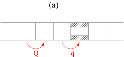
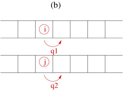
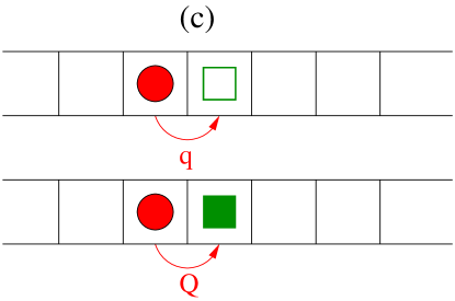
Figure 4: Schematic representation of the different types of randomness in particle-hopping models. In (a) the randomness is associated with the track; the hopping probability $q$ at the bottleneck (partially hatched region) is smaller than the normal hopping probability $Q$, In (b) the randomness is associated with the particles; $q_{1}$ and $q_{2}$ being the time-independent hopping probabilities of the particles $i$ and $j$, respectively. In (c) the randomness arises from the coupling of the dynamics of the hopping particles (filled circle) with another species of particles that represent specific type of signal molecules; the two possible states of the latter are represented by open and filled squares.

III.1 Modelling randomness in ASEP-type models

At least three different types of randomness of the hopping rates have been considered so far in the context of the ASEP-type models janowsky ; tripathy ; goldspeer ; krugdis ; evansdis ; ktitarev ; igloi .

(a) First, the randomness may be associated with the track on which the motile elements move janowsky ; tripathy ; goldspeer ; igloi ; typical examples are the bottlenecks created, in intra-cellular transport in neurons, by tau, a microtubule-associated protein mandeltau1 ; mandeltau2 . The inhomogeneities of some DNA and m-RNA strands can be well approximated as random kafri and, hence, the randomess of hopping of the motile elements on the nucleotide-based tracks. As shown schematically in fig.4(a), normal hopping probability at unblocked sites is $Q$ whereas that at the bottleneck is $q$ ($q<Q$). This type of randomness in the hopping probabilities, which may be treated as quenched (i.e., time-independent or “frozen”) defect of the track, leads to interesting phase-segregation phenomena (see css for a review).

(b) The second type of randomness is associated with the hopping motile elements krugdis ; evansdis ; ktitarev ; igloi , rather than with the track. For example, the normal hopping probabilities of the motile elements may vary randomly from one element to another (see fig.4(b)), e.g., in randomly mutated kinesins traffic ; hirotaked ; the hopping rate of each motile element is, however, “quenched”, i.e., independent of time. In this case, the system is known to be exhibit coarsening of queues of the motile elements and the phenomenon has some formal similarities with Bose-Einstein condensation (reviewed in css ). Note that in case of the randomness of type (a), the hopping probability depends only on the spatial location on the track, independent of the identity of the hopping motile element. On the other hand, in the case of randomness of type (b), the hopping probability depends on the hopping motile element, irrespective of its spatial location on the track.

(c) In contrast to the two types of randomness ((a) and (b)) considered above, the randomness in the hopping probabilities of the motile elements in some situations arises from the coupling of their dynamics with that of another non-conserved dynamical variable. For example, the hopping probability of a motile element may depend on the presence or absence of a specific type of signal molecule in front of it (see fig.4(c)); such situations arise in traffic of ants whose movements are strongly dependent on the presence or absence of pheromone on the trail ahead of them. Therefore, in such models with periodic boundary conditions, a given motile element may hop from the same site, at different times, with different hopping probabilities.

IV Generic mechanisms of single molecular motor

Two extremely idealized mechanisms of motility of single-motors have been developed in the literature. The power-stroke mechanism is analogous to the power strokes that drive macrscopic motors. On the other hand, the Brownian ratchet mechanism is unique to the microscopic molecular motors.

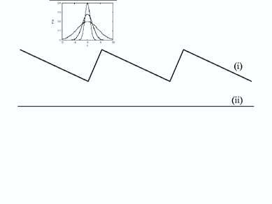
Figure 5: The two forms of the time-dependent potential used for implementing the Brownian ratchet mechanism. (Copyright: Indrani Chowdhury; reproduced with permission).

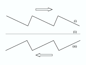
Figure 6: The direction of the motion of the particle in a Brownian ratchet, is determined by the form of the spatial asymmetry of the potential in each period when observed over times much longer than the time period of switching between the two forms of the potential. (Copyright: Indrani Chowdhury; reproduced with permission).

Let us now consider a Brownian particle subjected to a time-dependent potential, in addition to the viscous drag (or, frictional force). The potential switches between the two forms (i) and (ii) shown in fig.5. The sawtooth form (i) is spatially periodic where each period has an asymmetric shape. In contrast, the form (ii) is flat so that the particle does not experience any external force imposed on it when the potential has the form (ii). Note that, in the left part of each well in (i) the particle experiences a rightward force whereas in the right part of the same well it is subjected to a leftward force. Moreover, the spatially averaged force experienced by the particle in each well of length $\ell$ is

$$\langle F\rangle=-\frac{1}{\ell}\int_{0}^{\ell}\biggl{(}\frac{\partial U}{\partial x}\biggr{)}dx=U(0)-U(\ell)=0$$ (10)

because of the spatially periodic form of the potential (i). What makes this problem so interesting is that, in spite of vanishing average force acting on it, the particle can still exhibit directed, albeit noisy, rightward motion.

In order to understand the underlying physical principles, let us assume that initially the potential has the shape (i) and the particle is located at a point on the line that corresponds to the bottom of a well. Now the potential is switched off so that it makes a transition to the form (ii). Immediately, the free particle begins to execute a Brownian motion and the corresponding Gaussian profile of the probability distribution begins to spread with the passage of time. If the potential is again switched on before the Gaussian profile gets enough time for spreading beyond the original well, the particle will return to its original initial position. But, if the period during which the potential remains off is sufficiently long, so that the Gaussian probability distribution has a non-vanishing tail overlapping with the neighbouring well on the right side of the original well, then there is a small non-vanishing probability that the particle will move forward towards right by one period when the potential is switched on. In the case of cytoskeleton-based motors like kinesin and dynein, this energy is supplied by the hydrolysis of ATP molecules to ADP; thus, the mechanical movement is coupled to a chemical reaction.

In this mechanism, the particle moves forward not because of any force imposed on it but because of its Brownian motion. The system is, however, not in equilibrium because energy is pumped into it during every period in switching the potential between the two forms. In other words, the system works as a rectifier where the Brownian motion, in principle, could have given rise to both forward and backward movements of the particle in the multiples of $\ell$, but the backward motion of the particle is suppressed by a combination of (a) the time dependence and (b) spatial asymmetry (in form (i)) of the potential. In fact, the direction of motion of the particle can be reversed by replacing the potential (i) by the potential (iii) shown in fig.6. The spatial asymmetry of the sawtooth potential arises from the polar nature of the microtubule and actin filamentary tracks.

The mechanism of directional movement discussed above is called a Brownian ratchet julicher ; reimann . The concept of Brownian ratchet was popularized by Feynman through his lectures feynman although, historically, it was introduced by Smoluchowski smolurat .

IV.1 Modelling defects and disorder in Brownian ratchets

Effects of quenched (i.e., time-independent) disorder on the properties of Brownian ratchets have been considered by several authors harms ; marchesoni ; family ; kafri . Quenched disorder can arise in Brownian ratchets, for example, from
(i) random variation of the heights (or depths) of the sawtooth potential from one site to another where all the sawteeth have the same type of asymmetry,
(i) a random mixture of forward and reversed sawteeth where the heights of all the sawteeth is identical. The nature of disorder in real molecular motors, even if driven by a Brownian-ratchet mechanism, may be a combination of these two types of idealized disorder.

Suppose $\omega$ is the frequency of both the transitions from (i) to (ii) and (ii) to (i) forms of the potential. Also, let $P_{D}$ be the probability of finding a defect, i.e., a reversed sawtooth in case (ii). In that case, the effective drift and effective diffusion coefficient exhibit three different regions on the $P_{D}-\omega$ phase diagram harms including some anomalous behaviour.

V Intracellular transport: nucleotide-based motors

Helicases and polymerases are the two classes of nucleotide-based motors that have been the main focus of experimental investigations. In this section, we discuss only the motion of the ribosome along the m-RNA track. Historically, this problem is one of the first where TASP-like model was successfully applied to a biological system.

The synthesis of proteins and polypetids in a living cell is a complex process. Special machines, so-called ribosomes, translate the genetic information ‘stored’ in the messenger-RNA (mRNA) into a program for the synthesis of a protein. mRNA is a long (linear) molecule made up of a sequence of triplets of nucleotides; each triplet is called a codon. The genetic information is encoded in the sequence of codons. A ribosome, that first gets attached to the mRNA chain, “reads” the codons as it moves along the mRNA chain, recruits the corresponding amino acids and assembles these amino acids in the sequence so as to synthesize the protein for which the “construction plan” was stored in the mRNA. After executing the synthesis as per the plan, it gets detached from the mRNA. Thus, the process of “translation” of genetic information stored in mRNA consists of three steps: (i) initiation: attachment of a ribosome at the “start” end of the mRNA, (ii) elongation: of the polypeptide (protein) as the ribosome moves along the mRNA, and (iii) termination: ribosome gets detached from the mRNA when it reaches the “stop” codon.

Let us denote each of the successive codons by the successive sites of a one-dimensional lattice where the first and the last sites correspond to the start and stop codons. The ribosomes are much bigger (20-30 times) than the codons. Therefore, neighbouring ribosomes attached to the same mRNA can not read the same information or overtake each other. In other words, any given site on the lattice may be covered by a single ribosome or none. Let us represent each ribosome by a rigid rod of length $L_{r}$. If the rod representing the ribosome has its left edge attached to the i-th site of the lattice, it is allowed to move to the right by one lattice spacing, i.e., its left edge moves to the site $i+1$ provided the site $i+L_{r}$ is empty. In the special case $L_{r}=1$ this model reduced to the TASEP. Although the model was originally proposed in the late sixties macdonald , significant progress in its analytical treatment for the general case of arbitrary $L_{r}$ could be made only three decades later; even the effects of quenched disorder has also been considered in the recent literature shaw1 ; shaw2 ; shaw3 ; lakatos1 ; lakatos2 .

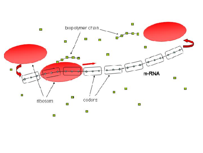
Figure 7: The process of biopolymerization: Ribosomes attach to mRNA and read the construction plan for a biopolymer which is stored in the genetic code formed by the sequence of codons. None of the codons can be read by more than one ribosome simultaneously.

As mentioned above, a ribosom is much bigger than a base triplet. However, modifying the ASEP by taking into account particles that occupy more than one lattice site does not change the structure of phase diagram macdonald . Physically this can be understood from the domain-wall picture and the extremal-current principle gunterrev ; schdom .

VI Intracellular transport: cytoskeleton-based motors

Intracellular transport is carried by molecular motors which are proteins that can directly convert the chemical energy into mechanical energy required for their movement along filaments constituting what is known as the cytoskeleton howard ; schliwa . Three superfamilities of these motors are kinesin, dynein and myosin. Members of the majority of the familities have two heads whereas only a few families have single-headed members. Most of the kinesins and dyneins are like porters in the sense that these move over long distances along the filamentary tracks without getting completely detached; such motors are called processive. On the other hand, the conventional myosins and a few unconventional ones are nonprocessive; they are like rowers. But, a few families of unconventional myosins are processive.

These cytoskeleton-based molecular motors play crucially important biological functions in axonal transport in neurons, intra-flagellar transport in eukaryotic flagella, etc. The relation between the architectural design of these motors and their transport function has been investigated both experimentally and theoretically for quite some time osterrev ; fisher ; astu1 .

However, in this review we shall focus mostly on the effects of mutual interactions (competition as well as cooperation) of these motors on their collective spatio-temporal organisation and the biomedical implications of such organisations. Often a single microtubule (MT) is used simultaneously by many motors and, in such circumstances, the inter-motor interactions cannot be ignored. Fundamental understanding of these collective physical phenomena may also expose the causes of motor-related diseases (e.g., Alzheimer’s disease) traffic ; hirotaked ; mandeld ; goldstein thereby helping, possibly, also in their control and cure. The bio-molecular motors have opened up a new frontier of applied research- “bio-nanotechnology”. A clear understanding of the mechanisms of these natural machines will give us clue as to the possible design principles that can be utilized to synthesize artificial nanomachines.

Derenyi and collaborators derenyi1 ; derenyi2 developed one-dimensional models of interacting Brownian motors, each of which is subjected to a time-dependent potential of the form shown in fig.5. They modelled each motor as a rigid rod and formulated the dynamics through Langevin equations of the form (2) for each such rod assuming the validity of the overdamped limit; the mutual interactions of the rods were incorporated through the mutual exclusion. However, in this section we shall focus attention on those models where the dynamics is formulated in terms of “rules” for undating in discrete time steps.

VI.1 TASEP-like generic models of molecular motor traffic

The model considered by Aghababaie et al.menon1 is not based on TASEP, but its dynamics is a combination of Brownian ratchet and update rules in discrete time steps. More precisely, this model is a generalization of TASEP, rather than TASEP, where the hopping probabilities are obtained from the local potential which itself is time-dependent and is assumed to have the form shown in fig.5.

In this model, the filamentary track is discretized in the spirit of the particle-hopping models described above and the motors are represented by field-driven particles; no site can accomodate more than one particle at a time. Each time step consists of either an attempt of a particle to hop to a neighbouring site or an attempt that can result in switching of the potential from flat to sawtooth form or vice-versa. Both forward and backward movement of the particles are possible and the hopping probability of every particle is computed from the instantaneous local potential. However, neither attachment of new particles nor complete detachment of existing particles were allowed.

The fundamental diagram of the model menon1 , computed imposing periodic boundary conditions, is very similar to those of TASEP. This observation indicates that further simplification of the model proposed in ref.menon1 is possible to develope a minimal model for interacting molecular motors. Indeed, the detailed Brownian ratchet mechanism, which leads to a noisy forward-directed movement of the field-driven particles in the model of Aghababaie et al. menon1 , is replaced in some of the more recent theoretical models lipo1 ; lipo2 ; lipo3 ; lipo4 ; lipo5 ; lipo6 ; lipo7 ; frey ; santen1 ; santen2 ; popkov1 by a TASEP-like probabilitic forward hopping of self-driven particles. In these simplied versions, none of the particles is allowed to hop backward and the forward hopping probability is assumed to capture most of the effects of biochemical cycle of the enzymatic activity of the motor. The explicit dynamics of the model is essentially an extension of that of the asymmetric simple exclusion processes (ASEP) sz ; gunterrev (see section III) that includes, in addition, Langmuir-like kinetics of adsorption and desorption of the motors.

$\bullet$ Model proposed by Parmeggiani et al.

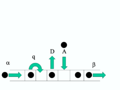
Figure 8: A schematic description of the TASEP-like model introduced in ref.frey for molecular motor traffic. Just as in TASEP, the motors are allowed to hop forward, with probability $q$. In addition, the motors can also get “attached” to an empty lattice site, with probability $A$, and “detached” from an occupied site, with probability $D$ from any site except the end points; the rate of attachment at the entry point on the left is $\alpha$ while that at the exit point on the right is $\beta$.

In the model of Parmeggiani et al. frey , the molecular motors are represented by particles whereas the sites for the binding of the motors with the cytoskeletal tracks (e.g., microtubules) are represented by a one-dimensional discrete lattice. Just as in TASEP, the motors are allowed to hop forward, with probability $q$, provided the site in front is empty. However, unlike TASEP, the particles can also get “attached” to an empty lattice site, with probability $A$, and “detached” from an occupied site, with probability $D$ (see fig.8) from any site except the end points. The state of the system was updated in a random-sequential manner.

Carrying out Monte-Carlo simulations of the model, applying open boundary conditions, Parmeggiani et al.frey demonstrated a novel phase where low and high density regimes, separated from each other by domain walls, coexist santen1 ; santen2 . Using a mean-field theory (MFT), they interpreted this spatial organization as traffic jam of molecular motors. This model has interesting mathematical properties sutapa which are of fundamental interest in statistical physics but are beyond the scope of this review.

$\bullet$ Model proposed by Klumpp et al.

Figure 9: A schematic description of the TASEP-like model introduced in ref.lipo1 for molecular motor traffic in a tubular geometry that mimics axonal transport. The thick axial line represents the microtubule track whereas the thin lines surrounding it merely indicate the non-directed diffusive channels of transport along the tube.

A cylindrical geometry of the model system (see fig.9) was considered by Lipowsky, Klumpp and collaborators lipo1 ; lipo2 ; lipo3 ; lipo4 ; lipo5 ; lipo6 ; lipo7 to mimic the microtubule tracks in typical tubular neurons. The microtubule filament was assumed to form the axis of the cylinder whereas the free space surrounding the axis was assumed to consist of $N_{ch}$ channels each of which was discretized in the spirit of lattice gas models. They studied concentration profiles and the current of free motors as well as those bound to the filament by imposing a few different types of boundary conditions. This model enables one to incorporate the effects of exchange of populations between two groups, namely, motors bound to the axial filament and motors which move diffusively in the cylinder. They have also compared the results of these investigations with the corresponding results obtained in a different geometry where the filaments spread out radially from a central point (see fig.10).

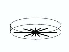
Figure 10: A schematic description of the TASEP-like model introduced in ref.lipo7 for intra-cellular molecular motor traffic in the radial geometry that mimics an aster.

$\bullet$ Model proposed by Klein et al.

It is well known that, in addition to generating forces and carrying cargoes, cytoskeletal motors can also depolymerize the filamentary track on which they move processively. A model for such filament depolymerization process has been developed by Klein et al.klein by extending the model of intra-cellular traffic proposed earlier by Parmeggiani et al. frey .

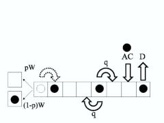
Figure 11: A schematic description of the model suggested by Klein et al. klein for motor induced depolymerization of cytoskeletal filaments. The lattice site at the tip of a filament is removed with a probability $W$ per unit time provided it is occupied by a motor; the motor remains attached to the newly exposed tip of the filament with probability $p$ (or remains bound with the removed site with probability $1-p$). The other symbols and procsses are identical to those shown in fig.8.

The model of Klein et al.klein is shown schematically in fig. 11. The novel feature of this model, in contrast to the similar models frey ; lipo7 ; santen1 of intracellular transport, is that the lattice site at the tip of a filament is removed with a probability $W$ per unit time provided it is occupied by a motor; the motor remains attached to the newly exposed tip of the filament with probability $p$ (or remains bound with the removed site with probability $1-p$). Thus, $p$ may be taken as a measure of the processivity of the motors. This model clearly demonstrated a dynamic accumulation of the motors at the tip of the filament arising from the processivity; a motor which was bound to the depolymerizing monomer at the tip of the filament is captured by the monomer at the newly exposed tip.

$\bullet$ Model proposed by Kruse and Sekimoto:

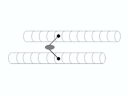
Figure 12: Schematic representation of Kruse and Sekimito’s model sekimoto for the motor-induced sliding of two cytoskeletal filaments. The cylinders represent the two filamentary tracks. The dark circles represent the two heads of a motor which are capable of binding on two binding sites on the two filaments provided the two binding sites are closest neighbours of each other. Each head can move forward following a TASEP-like rule and every movement of this type causes sliding of the two filaments by one single unit.

Kruse and Sekimoto sekimoto proposed a particle-hopping model for motor-induced relative sliding of two filamentary motor tracks. The model is shown schematically in fig.12. Each of the two-headed motors is assumed to consist of two particles connected to a common neck and are capable of binding with two filaments provided the two binding sites are closest neighbours as shown in the figure. Each particle can move forward following a TASEP-like rule and every movement of this type causes sliding of the two filaments by one single unit. The most important result of this investigation is that the average relative velocity of the filaments is a non-monotonic function of the concentration of the motors.

VI.2 Traffic of interacting single-headed motors KIF1A

The models of intracellular traffic described so far are essentially extensions of the asymmetric simple exclusion processes (ASEP) sz ; gunterrev that includes Langmuir-like kinetics of adsorption and desorption of the motors. In reality, a motor protein is an enzyme whose mechanical movement is loosely coupled with its biochemical cycle. In a recent work nishietal , we have considered specifically the single-headed kinesin motor, KIF1A okada1 ; okada2 ; okada3 ; Nitta ; unpub ; the movement of a single KIF1A motor was modelled earlier with a Brownian ratchet mechanism julicher ; reimann . In contrast to the earlier models frey ; santen1 ; popkov1 ; lipo7 of molecular motor traffic, which take into account only the mutual interactions of the motors, our model explicitly incorporates also the Brownian ratchet mechanism of individual KIF1A motors, including its biochemical cycle that involves adenosine triphosphate(ATP) hydrolysis.

The ASEP-like models successfully explain the occurrence of shocks. But since most of the bio-chemistry is captured in these models through a single effective hopping rate, it is difficult to make direct quantitative comparison with experimental data which depend on such chemical processes. In contrast, the model we proposed in ref. nishietal incorporates the essential steps in the biochemical processes of KIF1A as well as their mutual interactions and involves parameters that have one-to-one correspondence with experimentally controllable quantities.

The biochemical processes of kinesin-type molecular motors can be described by the four states model shown in Fig. 13 okada1 ; Nitta : bare kinesin (K), kinesin bound with ATP (KT), kinesin bound with the products of hydrolysis, i.e., adenosine diphosphate(ADP) and phosphate (KDP), and, finally, kinesin bound with ADP (KD) after releasing phosphate. Recent experiments okada1 ; Nitta revealed that both K and KT bind to the MT in a stereotypic manner (historically called “strongly bound state”, and here we refer to this mechanical state as “state 1”). KDP has a very short lifetime and the release of phosphate transiently detaches kinesin from MT Nitta . Then, KD re-binds to the MT and executes Brownian motion along the track (historically called “weakly bound state”, and here referred to as “state 2”). Finally, KD releases ADP when it steps forward to the next binding site on the MT utilizing a Brownian ratchet mechanism, and thereby returns to the state K.

Figure 13: The biochemical and mechanical states of a single KIF1A motor. In the chemical states on the left of the dotted line, KIF1A binds to a fixed position on the MT (state 1), while in those on the right KIF1A diffuses along the MT track (state 2). At the transition from state 1 to 2, KIF1A detaches from the MT.

Thus, in contrast to the earlier ASEP-like models, each of the self-driven particles, which represent the individual motors KIF1A, can be in two possible internal states labelled by the indices $1$ and $2$. In other words, each of the lattice sites can be in one of three possible allowed states (Fig. 14): empty (denoted by $0$), occupied by a kinesin in state $1$, or occupied by a kinesin in state $2$.

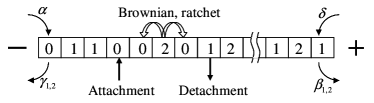
Figure 14: A 3-state model for molecular motors moving along a MT. 0 denotes an empty site, 1 is K or KT and 2 is KD. Transition from 1 to 2, which corresponds to hydrolysis, occurs within a cell whereas movement to the forward or backward cell occurs only when motor is in state 2. At the minus and plus ends the probabilities are different from those in the bulk.

For the dynamical evolution of the system, one of the $L$ sites is picked up randomly and updated according to the rules given below together with the corresponding probabilities (Fig. 14):

$${\rm Attachment:}\,\,\,\,\,0\to 1\,\,\,{\rm with}\,\,\omega_{a}dt$$ (11)

$${\rm Detachment:}\,\,\,\,1\to 0\,\,\,{\rm with}\,\,\ \omega_{d}dt$$ (12)

$${\rm Hydrolysis:}\,\,\,\,\,1\to 2\,\,\,{\rm with}\,\,\omega_{h}dt$$ (13)

$${\rm Ratchet:}\,\,\,\,\,\left\{\begin{array}[]{c}2\to 1\,\,\,{\rm with}\,\,\omega_{s}dt\\ 20\to 01\,\,\,{\rm with}\,\,\omega_{f}dt\end{array}\right.$$ (16)

$${\rm Brownian\ motion:}\,\,\,\,\,\left\{\begin{array}[]{c}20\to 02\,\,\,{\rm with}\,\,\omega_{b}dt\\ 02\to 20\,\,\,{\rm with}\,\,\omega_{b}dt\end{array}\right.$$ (19)

The probabilities of detachment and attachment at the two ends of the MT may be different from those at any bulk site. We chose $\alpha$ and $\delta$, instead of $\omega_{a}$, as the probabilities of attachment at the left and right ends, respectively. Similarly, we took $\gamma_{1}$ and $\beta_{1}$, instead of $\omega_{d}$, as probabilities of detachments at the two ends (Fig. 14). Finally, $\gamma_{2}$ and $\beta_{2}$, instead of $\omega_{b}$, are the probabilities of exit of the motors through the two ends by random Brownian movements.

It is possible to relate the rate constants $\omega_{f}$, $\omega_{s}$ and $\omega_{b}$ with the corresponding physical processes in the Brownian ratchet mechanism of a single KIF1A motor. Suppose, just like models of flashing ratchets julicher ; reimann , the motor “sees” a time-dependent effective potential which, over each biochemical cycle, switches back and forth between (i) a periodic but asymmetric sawtooth like form and (ii) a constant. The rate constant $\omega_{h}$ in our model corresponds to the rate of the transition of the potential from the form (i) to the form (ii). The transition from (i) to (ii) happens soon after ATP hydrolysis, while the transition from (ii) to (i) happens when ATP attaches to a bare kinesinokada1 . The rate constant $\omega_{b}$ of the motor in state $2$ captures the Brownian motion of the free particle subjected to the flat potential (ii). The rate constants $\omega_{s}$ and $\omega_{f}$ are proportional to the overlaps of the Gaussian probability distribution of the free Brownian particle with, respectively, the original well and the well immediately in front of the original well of the sawtooth potential.

Good estimates for the parameters of the model could be extracted by analyzing the empirical data nishietal . For example, $\omega_{d}\simeq 0.0001$ ms^-1 is independent of the kinesin concentration. On the other hand, $\omega_{a}$, which depends on the kinesin concentration, could be in the range $0.0001$ ms${}^{-1}\leq\omega_{a}\leq 0.01$ ms^-1. Similarly, $\omega_{b}\simeq 0.6$ ms^-1, $\omega_{s}\simeq 0.145$ ms^-1, $\omega_{f}\simeq 0.055$ ms^-1 and $0\leq\omega_{h}\leq 0.25$ ms^-1.

Let us denote the probabilities of finding a KIF1A molecule in the states $1$ and $2$ at the lattice site $i$ at time $t$ by the symbols $r_{i}$ and $h_{i}$, respectively. In mean-field approximation the master equations for the dynamics of motors in the bulk of the system are given by

$$\frac{dr_{i}}{dt} = \omega_{a}(1-r_{i}-h_{i})-\omega_{h}r_{i}-\omega_{d}r_{i}+\omega_{s}h_{i}+\omega_{f}h_{i-1}(1-r_{i}-h_{i}),$$ (20)

$$\frac{dh_{i}}{dt} = -\omega_{s}h_{i}+\omega_{h}r_{i}-\omega_{f}h_{i}(1-r_{i+1}-h_{i+1})$$ (21)

$$-\omega_{b}h_{i}(2-r_{i+1}-h_{i+1}-r_{i-1}-h_{i-1})+\omega_{b}(h_{i-1}+h_{i+1})(1-r_{i}-h_{i}).$$

The corresponding equations for the boundaries are also similar unpub .

ATP (mM)	$\omega_{h}$ (1/ms)	$v$ (nm/ms)	$D/v$ (nm)	$\tau$ (s)
$\infty$	0.25	0.201	184.8	7.22
0.9	0.20	0.176	179.1	6.94
0.3375	0.15	0.153	188.2	6.98
0.15	0.10	0.124	178.7	6.62

Table 1: Predicted transport properties from our model nishietal in the low-density limit for four different ATP concentrations. $\tau$ is calculated by averaging the intervals between attachment and detachment of each KIF1A.

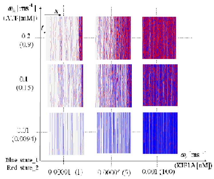
Figure 15: Phase diagram of our model nishietal in the $\omega_{h}-\omega_{a}$ plane, with the corresponding values for ATP and KIF1A concentrations given in brackets. These quantities are controllable in experiment. The boundary rates are $\alpha=\omega_{a},\beta_{1,2}=\omega_{d},\gamma_{1,2}=\delta=0$. The position of the immobile shock depends on both ATP and KIF1A concentrations.

Assuming that each time step of updating corresponds to 1 ms of real time, we performed simulations upto 1 minute. In the limit of low density of the motors we have computed, for example, the mean speed of the kinesins, the diffusion constant and mean duration of the movement of a kinesin on a microtubule from simulations of our model (see table 1); these are in excellent quantitative agreement with the corresponding empirical data from single molecule experiments.

Using this model we have also calculated the flux of the motors in the mean field approximation imposing periodic boundary conditions. Although the system with periodic boundary conditions is fictitious, the results provide good estimates of the density and flux in the corresponding system with open boundary conditions.

In contrast to the phase diagrams in the $\alpha-\beta$-plane reported by earlier investigators frey ; santen1 ; lipo7 , we have drawn the phase diagram of our model in the $\omega_{a}-\omega_{h}$ plane (see fig.15) by carrying out extensive computer simulations for realistic parameter values of the model with open boundary conditions. The phase diagram shows the strong influence of hydrolysis on the spatial distribution of the motors along the MT. For very low $\omega_{h}$ no kinesins can exist in state 2; the kinesins, all of which are in state 1, are distributed rather homogeneously over the entire system. In this case the only dynamics present is due to the Langmuir kinetics. At a small, but finite, rate $\omega_{h}$ both the density profiles $\rho_{j}^{1}$ and $\rho_{j}^{2}$ of kinesins in the states 1 and 2 exhibit a localized shock. Interestingly, the shocks in these two density profiles always appear at the same position. Moreover, the position of the immobile shock depends on the concentration of the motors as well as that of ATP; the shock moves towards the minus end of the MT with the increase of the concentration of kinesin or ATP or both (Fig. 15).

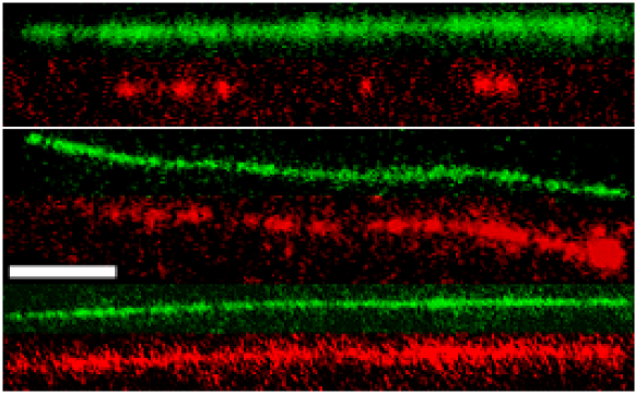
Figure 16: Formation of comet-like accumulation of kinesin at the end of MT. Fluorescently labeled KIF1A (red) was introduced to MT (green) at 10 pM (top), 100 pM (middle) and 1000 pM (bottom) concentrations along with 2 mM ATP. The length of the white bar is 2$\mu m$.

The formation of the shock has been established by our direct experimental evidence. The “comet-like structure”, shown in the middle of Fig. 16, is the collective pattern formed by the red fluorescent labelled kinesins where a domain wall separates the low-density region from the high-density region. The position of the domain wall depends on both ATP and KIF1A concentrations. Our findings on the domain wall are in qualitative agreement with the corresponding experimental observations.

VII Extracellular transport: collagen-based motors

The extracellular matrix (ECM) nagase of vertebrates is rich in collagen. Monomers of collagen form a triple-helical structure which self-assemble into a tightly packed periodic organization of fibrils. Cells residing in tissues can secret matrix metalloproteases (MMPs), a special type of enzymes that are capable of degrading macromolecular constituents of the ECM. The most notable among these enzymes is MMP-1 that is known to degrade collagen. The collagen fibril contains cleavage sites which are spaced at regular intervals of $300$ nm. The collagenase MMP-1 cleaves all the three $\alpha$ chains of the collagen monomer at a single site.

Figure 17: Schematic representation of the two-dimensional burnt bridge model of MMP-1 dynamics. Each triangle represents a MMP-1 and the erased segments represent the “degraded” segments of the collagen fibril.

Breakdown of the ECM forms an essential step in several biological processes like, for example, embryonic development, tissue remodelling, etc. nagase . Malfunctioning of MMP-1 has been associated with wide range of diseases whittaker . Therefore, an understanding of the MMP-1 traffic on collagen fibrils can provide deeper insight into the mechanism of its operation which, in turn, may give some clue as to the strategies of control and cure of diseases caused by the inappropriate functions of these enzymes.

VII.1 Phenomenology of MMP-1 dynamics

Saffarian et al. saffarian used a technique of two-photon excitation fluorescence correlation spectroscopy to measure the correlation function corresponding to the MMP-1 moving along the collagen fibrils. The measured correlation function strongly indicated that the motion of the MMP-1 was not purely diffusive, but a combination of diffusion and drift. In other words, the “digestion” of a collagen fibril occurs when a MMP-1 executes a biased diffusion processively (i.e., without detachment) along the fibril. They also demonstrated that inactivation of the enzyme eliminates the bias but the diffusion remains practically unaffected. They claimed that the energy required for the active motor-like transport of the MMP-1 comes from the proteolysis (i.e., degradation) of the collagen fibrils.

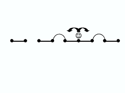
Figure 18: Schematic representation of the one-dimensional burnt bridge model of MMP-1 dynamics proposed in ref.blumen . The thick straight lines cannot be burnt whereas the thin arches can get burnt by the random walker (see the text for details of the dynamics). The erased links represent the burnt bridges.

Saffarian et al. saffarian also carried out computer simulations of a two-dimensional model of the MMP-1 dynamics on collagen fibrils; this model is a generalization of the one-dimensional “burnt bridge model” introduced earlier by Mai et al. blumen . (We shall discuss this model in the next subsection). By comparing the results of these simulations with their experimental observations, Saffarian et al. they concluded that the observed biased diffusion of the MMP-1 on collagen fibrils can be described quite well by a Brownian ratchet mechanism julicher ; reimann .

VII.2 A stochastic burnt-bridge model of MMP-1 dynamics

A one-dimensional “burnt-bridge” model was developed by Mai et al. blumen to demonstrate a novel mechanism of directed transport of a Brownian particle. The model is sketched schematically in fig.18. A “particle” performs a random walk on a semi-infinite one-dimensional lattice that extends from the origin to $+\infty$. Each site of the lattice is connected to the two nearest neighbour sites by links; a fraction $c$ of these links are called “bridges” and these are prone to be burnt by the random walker. A bridge is burnt, with probability $p$, if the random walker either crosses it from left to right or attempts to cross if from right to left blumen ; antal . In either case, if the bridge is actually burnt, the walker stays on the right of the burnt bridge and cannot cross it any more. The hindrance against leftward motion, that is created by the burnt bridges, is responsible for the overall rightward drift of the random walker.

Mai et al.blumen studied the dependence of the average drift velocity $v$ on the parameters $p$ and $c$ by computer simulation. They also derived approximate analytical forms of these dependences in the two limits $p\ll 1$ and $p\simeq 1$ using a continuum approximation.

Almost every event of crossing of a bridge from left to right or attempt of crossing from right to left burns the bridge in the limit $p\simeq 1$. Whenever the walker burns a bridge, it can take the right edge of the burnt bridge as the new origin. Thus, every event of burning of a bridge defines a new segment of the lattice having a burnt bridge at its left end and a intact bridge at its right end. The random walker performs its diffusive movement in the segment such that there is a reflecting boundary for the random walker at the left end of the segment and an absorbing boundary at the right end of the segment. If the bridges were equispaced, each of these segments will have a length $\ell=1/c$. Therefore, $\tau$, the time taken to cross the distance $\ell$ will be given by $\ell^{2}=2D\tau$ and, hence, the corresponding speed of the walker $v=\ell/\tau=2D/\ell=2cD$. Mai et al. argued that if the bridges are intially distributed randomly, the average speed will be reduced to $v=cD$. Thus, in the limit $p\rightarrow 1$, $v\propto c$. In contrast, in the limit $p\ll 1$, they found $v\propto\sqrt{pc}$.

VIII Cellular traffic

A Mycoplasma mobile (MB) bacterium is an uni-cellular organism. Each of the pear-shaped cells of this bacterium is about $700$ nm long and has a diameter of about $250$ nm at the widest section. Each bacterium can move fast on glass or plastic surfaces using a gliding mechanism.

In a recent experiment hiratsuka narrow linear channels were constructed on lithographic substrates. The channels were typically $500$ nm wide and $800$ nm deep. Note that each chennel was approximately twice as wide as the width of a single MB cell (see the sketch on the left side of the fig.19). The channels were so deep that none of the individual MB cells was able to climb up the tall walls of the channels and continued moving along the bottom edge of the walls of the cannels. In the absence of direct contact interaction with other bacteria, each individual MB cell was observed to glide, without changing direction, at an average speed of a few microns per second.

When two MB cells made a contact approaching each other from opposite directions within the same channel, one of the two cells gave way and moved to the adjacent lane. However, in a majority of the cases, two cells approaching each other from the opposite directions simply passed by as if nothing had happened; this is because of the fact that the width of the chennel is roughly twice that of the individual MB cell. Moreover, when two cells moving in the same direction within a channel collided with each other, the faster cell moved to the adjacent lane after the collision.

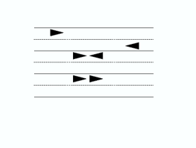
Figure 19: Schematic description of the traffic flow of Mycoplasma (represented by the triangles) in (a) the expertment of Hiratsuka et al. (b) the single-channel model of Vartak et al. vartak . The width of each channel in both (a) and (b) is just enough to allow the passage of two cells side by side. Both uni-directional and bi-directional traffic are possible.

Hiratsuka et al.hiratsuka attached micron-sized beads on the MB cells using biochemical technique and demonstrated that the average speed of each MB cell remained practically unaffected by the load it was carrying. In contrast to the nonliving motile elements discussed in all the preceedings sections, the cells are the functional units of life. Therefore, the MB cells have the potential for use in applied research and technology as “micro-transporters”. More recently, the unicellular biflagellated algae Chlamydomonas reinhardtii (CR), which are known to be phototactic swimmers, have been shown to be even better cadidates as “micro-transporter” as these can attain average speeds that is about two orders of magnitude higher than what was possible with MB cells weibel . However, to our knowledge, the effects of mutual interactions of the CR cells on their average speed at higher densities has not been investigated.

IX Traffic in social insect colonies: ants and termites

From now onwards, in this review we shall study traffic of multi-cellular organisms. We begin with the simpler (and smaller) organisms and, then, consider those of organisms with larger sizes and more complex physiology in the next section.

Termites, ants, bees and wasps are the most common social insects, although the extent of social behavior, as compared to solitary life, varies from one sub-species to another wilson . The ability of the social insect colonies to function without a leader has attracted the attention of experts from different disciplines bonabu97 ; anderson02 ; huang ; bonabu98 ; theraulaz03 ; gautrais ; keshet94 ; theraulazetal . Insights gained from the modeling of the colonies of such insects are finding important applications in computer science (useful optimization and control algorithms) dorigo , communication engineering bona00 , artificial “swarm intelligence” bonabeau and micro-robotics krieger as well as in task partitioning, decentralized manufacturing anderson99a ; anderson99b ; anderson99c ; anderson00a ; anderson01 ; anderson00b and management meyer .

In this section we consider only ants as the collective terrestrial movements of these have close similarities with the other traffic-like phenomena considered here. When observed from a sufficiently long distance the movement of ants on trails resemble the vehicular traffic observed from a low flying aircraft.

Ants communicate with each other by dropping a chemical (generically called pheromone) on the substrate as they move forward wilson ; camazine ; mikhailov . Although we cannot smell it, the trail pheromone sticks to the substrate long enough for the other following sniffing ants to pick up its smell and follow the trail. This process is called chemotaxis wilson .

Rauch et al.rauch developed a continuum model, following a hybrid of the individual-based and population-based approaches in terms of an effective energy landscape. They wrote one set of stochastic differential equations for the positions of the ants and another set of PDEs for the local densities of pheromone. Both this model and the CA model introduced by Watmough and Edelstein-Keshet watmough were intended to address the question of formation of the ant-trail networks by foraging ants.

Couzin and Franks couzin developed an individual based model that not only addressed the question of self-organized lane formation but also elucidated the variation of the flux of the ants with two important parameters of the model. The “internal angle” $\alpha$ may be interpreted as angle of local visual field or that of olfactory perception, or tactile range of the antennae of the individual ants. Moreover, each individual ant is assumed to turn away from others within these zones by, at most, an angle $\theta_{a}\Delta t$ in time $\Delta t$.

Imposing periodic boundary conditions, Couzin and Franks couzin computed the flux of ants in their model by computer simulations. The flux was found to be a nonmonotinic function of both $\alpha$ and $\theta_{a}$. At low $\alpha$, ants cannot detect others ahead whereas at high $\alpha$ they spend most of their time avoiding others even through collisions with others may be unlikely; both these reduce the flux considerably. Similarly, at low $\theta_{a}$ ants cannot turn sufficiently rapidly to avoid collision whereas at high $\theta$ they change their direction quickly so that not many move in the same direction at any time. Thus, only in the intermediate range of values of $\alpha$ and $\theta_{a}$, the ants are optimally sensitive. Therefore, the flux exhibits a maximum both as a function of $\alpha$ and as a function of $\theta_{a}$.

In the recent years, we have developed discrete models that are not intended to address the question of the emergence of the ant-trail activewalker , but focus on the traffic of ants on a trail which has already been formed. We have developed models of both unidirectional and bidirectional ant-traffic by generalizing the totally asymmetric simple exclusion process (TASEP) derrida1 ; derrida2 ; gunterrev with parallel dynamics by taking into account the effect of the pheromone.

IX.1 Model of single-lane uni-directional ant-traffic

In our model of uni-directional ant-traffic the ants move according to a rule which is essentially an extension of the TASEP dynamics. In addition, a second field is introduced which models the presence or absence of pheromones (see Fig. 20). The hopping probability of the ants is now modified by the presence of pheromones. It is larger if a pheromone is present at the destination site. Furthermore, the dynamics of the pheromones has to be specified. They are created by ants and free pheromones evaporate with probability $f$ per unit time. Assuming periodic boundary conditions, the state of the system is updated at each time step in two stages (see Fig. 20). In stage I ants are allowed to move while in stage II the pheromones are allowed to evaporate. In each stage the stochastic dynamical rules are applied in parallel to all ants and pheromones, respectively.

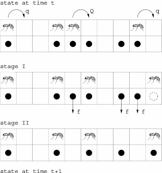
Figure 20: Schematic representation of typical configurations of the uni-directional ant-traffic model. The symbols $\bullet$ indicate the presence of pheromone. This figure also illustrates the update procedure. Top: Configuration at time $t$, i.e. before stage I of the update. The non-vanishing probabilities of forward movement of the ants are also shown explicitly. Middle: Configuration after one possible realisation of stage I. Two ants have moved compared to the top part of the figure. The open circle with dashed boundary indicates the location where pheromone will be dropped by the corresponding ant at stage II of the update scheme. Also indicated are the existing pheromones that may evaporate in stage II of the updating, together with the average rate of evaporation. Bottom: Configuration after one possible realization of stage II. Two drops of pheromones have evaporated and pheromones have been dropped/reinforced at the current locations of the ants.

(a)

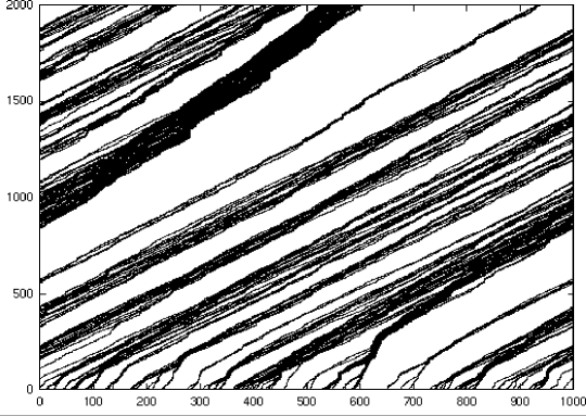
(b)

Figure 21: Snapshots of the spatial configurations demonstrating coarsening of the clusters of ants (a) in the early stages and (b) in the late stages of time evolution starting from random initial condition. The position of each ant is denoted by a black dot. A horizontal row of dots on such space-time plots denotes the positions of the ants (i.e., a snapshot of the system) at a given instant of time; an upper row corresponds to the snapshot at a later time.

Stage I: Motion of ants
An ant in a site cannot move if the site immediately in front of it is also occupied by another ant. However, when this site is not occupied by any other ant, the probability of its forward movement to the ant-free site is $Q$ or $q$, depending on whether or not the target site contains pheromone. Thus, $q$ (or $Q$) would be the average speed of a free ant in the absence (or presence) of pheromone. To be consistent with real ant-trails, we assume $q<Q$, as presence of pheromone increases the average speed.

Stage II: Evaporation of pheromones
Trail pheromone is volatile. So, pheromone secreted by an ant will gradually decay unless reinforced by the following ants. In order to capture this process, we assume that each site occupied by an ant at the end of stage I also contains pheromone. On the other hand, pheromone in any ‘ant-free’ site is allowed to evaporate; this evaporation is also assumed to be a random process that takes place at an average rate of $f$ per unit time.

The total amount of pheromone on the trail can fluctuate although the total number $N$ of the ants is constant because of the periodic boundary conditions. In the two special cases $f=0$ and $f=1$ the stationary state of the model becomes identical to that of the TASEP with hopping probability $Q$ and $q$, respectively.

One interesting phenomenon observed in the simulations is coarsening. At intermediate time usually several non-compact clusters are formed (Fig. 21(a)). However, the velocity of a cluster depends on the distance to the next cluster ahead. Obviously, the probability that the pheromone created by the last ant of the previous cluster survives decreases with increasing distance. Therefore clusters with a small headway move faster than those with a large headway. This induces a coarsening process such that after long times only one non-compact cluster survives (Fig. 21(b)). A similar behaviour has been observed also in the bus-route model loan ; cd . If the system evolves from a random initial condition at $t=0$, then during coarsening of the cluster, its size $R(t)$ at time $t$ is given by $R(t)\sim t^{1/2}$ loan ; cd .

  

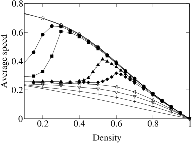
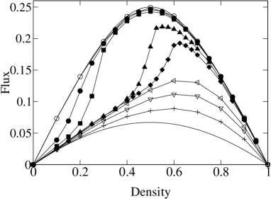
Figure 22: The variation of the average speed (left) and flux (right) of the ants with their density on trail.

In vehicular traffic, usually, the inter-vehicle interactions tend to hinder each other’s motion so that the average speed of the vehicles decreases monotonically with increasing density. In contrast, in our model of uni-directional ant-traffic the average speed of the ants varies non-monotonically with their density over a wide range of small values of $f$ because of the coupling of their dynamics with that of the pheromone (see fig.22). This uncommon variation of the average speed gives rise to the unusual dependence of the flux on the density of the ants in our uni-directional ant-traffic model (see fig.22). Furthermore, the flux is no longer particle-hole symmetric.

IX.2 Model of single-lane bi-directional ant-traffic

The single-lane model of uni-directional ant traffic, which we have discussed above, has been extended kunwar to capture the essential features of bi-directional ant-traffic in some special situations like, for example, on hanging cables (see fig.23).

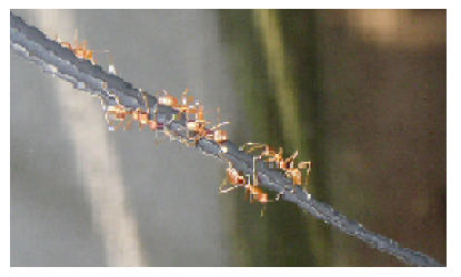
Figure 23: A snapshot of an ant-trail on a hanging cable. It can be regarded as strictly one-dimensional. But, nevertheless, traffic flow in opposite directions is possible as two ants, which face each other on the upper side of the cable, can exchange their positions if one of them, at least temporarily, switches over to the lower side of the cable.

initial	final	rate
RL	RL	$1-K$
	LR	$K$
RP	RP	$(1-f)(1-Q)$
	R0	$f(1-Q)$
	0R	$fQ$
	PR	$(1-f)Q$
R0	R0	$1-q$
	0R	$fq$
	PR	$(1-f)q$

initial	final	rate
PR	PR	$1-f$
	0R	$f$
P0	P0	$1-f$
	00	$f$
PP	PP	$(1-f)^{2}$
	P0	$f(1-f)$
	0P	$f(1-f)$
	00	$f^{2}$

Figure 24: Nontrivial transitions and their transition rates in the PRL model kunwar . Transitions from initial states $PL$, $0L$ and $0P$ are not listed. They can be obtained from those for $LP$, $L0$ and $P0$, respectively, by replacing $R\leftrightarrow L$ and, then, taking the mirror image.

In our model the right-moving (left-moving) particles, represented by $R$ ($L$), are never allowed to move towards left (right); these two groups of particles are the analogs of the outbound and nest-bound ants in a bi-directional traffic on the same trail. Thus, no U-turn is allowed. In addition to the TASEP-like hopping of the particles onto the neighboring vacant sites in the respective directions of motion, the $R$ and $L$ particles on nearest-neighbour sites and facing each other are allowed to exchange their positions, i.e., the transition $RL\overset{K}{\to}~{}~{}LR$ takes place, with the probability $K$. This might be considered as a minimal model for the motion of ants on a hanging cable as shown in Fig.23. When a outbound ant and a nest-bound ant face each other on the upper side of the cable, they slow down and, eventually, pass each other after one of them, at least temporarily, switches over to the lower side of the cable. Similar observations have been made for normal ant-trails where ants pass each other after turning by a small angle to avoid head-on collision couzin ; burd2 . In our model, as commonly observed in most real ant-trails, none of the ants is allowed to overtake another moving in the same direction.

We now introduce a third species of particles, labelled by the letter $P$, which are intended to capture the essential features of pheromone. The $P$ particles are deposited on the lattice by the $R$ and $L$ particles when the latter hop out of a site; an existing $P$ particle at a site disappears when a $R$ or $L$ particle arrives at the same location. The $P$ particles cannot hop but can evaporate, with a probability $f$ per unit time, independently from the lattice. None of the lattice sites can accomodate more than one particle at a time.

The state of the system is updated in a random-sequential manner. Because of the periodic boundary conditions, the densities of the $R$ and the $L$ particles are conserved. In contrast, the density of the $P$ particles is a non-conserved variable. The distinct initial states and the corresponding final states for pairs of nearest-neighbor sites are shown in fig.24 together with the respective transition probabilties.

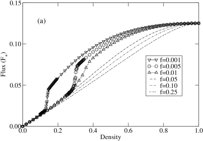
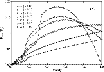
Figure 25: The fundamental diagrams in the steady-state of the PRL model kunwar for several different values of (a) $f$ (for $\phi=0.5$) and (b) $\phi$ (for $f=0.001$). The other common parameters are $Q=0.75,q=0.25$, $K=0.5$ and $M=1000$. Non-monotonic variation of the average speeds of the ants with their density on the trail gives rise to the unusual shape of the fundamental diagrams.

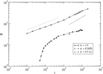
Figure 26: Average size of the cluster $R$ in the PRL model kunwar is plotted against time $t$ for $\phi=1.0$, and $\phi=0.5$, both for the same total density $c=0.2$; the other common parameters being $Q=0.75$, $q=0.25$, $K=0.50$, $f=0.005$, $M=4000$.

Suppose $N_{+}$ and $N_{-}=N-N_{+}$ are the total numbers of $R$ and $L$ particles, respectively. For a system of length $M$ the corresponding densities are $c_{\pm}=N_{\pm}/M$ with the total density $c=c_{+}+c_{-}=N/M$. Of the $N$ particles, a fraction $\phi=N_{+}/N=c_{+}/c$ are of the type $R$ while the remaining fraction $1-\phi$ are $L$ particles. The corresponding fluxes are denoted by $J_{\pm}$. In both the limits $\phi=1$ and $\phi=0$ this model reduces to the model reported in ref.cgns ; ncs and reviewed in section IX.A, which was motivated by uni-directional ant-traffic and is closely related to the bus-route models loan ; cd .

One unusual feature of this PRL model is that the flux does not vanish in the dense-packing limit $c\rightarrow 1$. In fact, in the full-filling limit $c=1$, the exact non-vanishing flux $J_{+}=Kc_{+}c_{-}=J_{-}$ at $c_{+}+c_{-}=c=1$ arises only from the exchange of the $R$ and $L$ particles, irrespective of the magnitudes of $f,Q$ and $q$.

In the special case $Q=q=:q_{h}$ the hopping of the ants become independent of pheromone. This special case of the PRL model is identical to the AHR model arndt with $q_{-}=0=\kappa$. A simple mean-field approximation (MFA) yields the estimates

$$J_{\pm}\simeq c_{\pm}\biggl{[}q_{h}(1-c)+Kc_{\mp}\biggr{]}$$ (22)

irrespective of $f$, for the fluxes $J_{\pm}$ at any arbitrary $c$. We found that the results of MFA agree reasonably well with the exact values of the flux rajewsky for all $q_{h}\geq 1/2$ but deviate more from the exact values for $q_{h}<1/2$, indicating the presence of stronger correlations at smaller values of $q_{h}$.

For the generic case $q\neq Q$, the flux in the PRL model depends on the evaporation rate $f$ of the $P$ partcles. In Fig. 25 we plot the fundamental diagrams for wide ranges of values of $f$ (in Fig. 25(a)) and $\phi$ (in Fig. 25(b)), corresponding to one set of hopping probabilities. First, note that the data in figs. 25 are consistent with the physically expected value of $J_{\pm}(c=1)=Kc_{+}c_{-}$, because in the dense packing limit only the exchange of the oppositely moving particles contributes to the flux. Moreover, the sharp rise of the flux over a narrow range of $c$ observed in both Fig. 25 (a) and (b) arise from the nonmonotonic variation of the average speed with density, an effect which was also observed in our earlier model for uni-directional ant traffic cgns ; ncs .

In the special limits $\phi=0$ and $\phi=1$, this model reduces to our single-lane model of unidirectional ant traffic; therefore, in these limits, over a certain regime of density (especially at small $f$), the particles are expected cgns ; ncs to form “loose” (i.e., non-compact) clusters ncs . Therefore, in the absence of encounter with oppositely moving particles, $\tau_{\pm}$, the coarsening time for the right-moving and left-moving particles would grow with system size as $\tau_{+}\sim\phi^{2}M^{2}$ and $\tau_{-}\sim(1-\phi)^{2}M^{2}$.

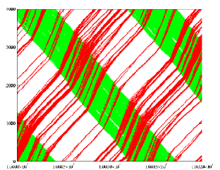
Figure 27: Space-time plot of the PRL model for $Q=0.50$, $q=0.25$, $f=0.005$, $c=0.2$, $\phi=0.3$, $K=1.0$ and $M=4000$. The black and grey dots represent the right-moving and left-moving ants, respectively.

In the PRL model with periodic boundary conditions, the oppositely moving ‘loose” clusters “collide” against each other periodically where the time gap $\tau_{g}$ between the successive collisions increases linearly with the system size following $\tau_{g}\sim M$; we have verified this scaling relation numerically (see the typical space-time diagram in fig.27). During a collision each loose cluster “shreds” (i.e., cuts into pieces) the oppositely moving cluster; both clusters shred the other equally if $\phi=1/2$. However, for all $\phi\neq 1/2$, the minority cluster suffers more severe shredding than that suffered by the majority cluster because each member of a cluster contributes in the shredding of the oppositely moving cluster. In small systems the “shredded” clusters get opportunity for significant re-coarsening before getting shredded again in the next encounter with the oppositely moving particles. But, in sufficiently large systems, shredded appearance of the clusters persists. However, we observed practically no difference in the fundamental diagrams for $M=1000$ and $M=4000$.

Following the methods of ref.cd , we have computed $R(t)$ starting from random initial conditions. The data (Fig. 26(a)) corresponding to $\phi=1$ are consistent with the asymptotic growth law $R(t)\sim t^{1/2}$. In sharp contrast, for $\phi=0.5$, $R(t)$ saturates to a much smaller value (Fig. 26(b)) that is consistent with highly shredded appearance of the corresponding clusters.

Thus, coarsening and shredding phenomena compete against each other and this competition determines the overall spatio-temporal pattern. Therefore, in the late stage of evolution, the system settles to a state where, because of alternate occurrence of shredding and coarsening, the typical size of the clusters varies periodically. Moreover, we find that, for given $c$ and $\phi$, increasing $K$ leads to sharper speeding up of the clusters during collision so long as $K$ is not much smaller than $q$. Both the phenomena of shredding and speeding during collisions of the oppositely moving loose clusters arise from the fact that, during such collisions, the domainant process is the exchange of positions, with probability $K$, of oppositely-moving ants that face each other.

IX.3 Model of two-lane bi-directional ant-traffic

It is possible to extend the model of uni-directional ant-traffic to a minimal model of two-lane bi-directional ant-traffic jscn . In such models of bi-directional ant-traffic the trail consists of two lanes of sites. These two lanes need not be physically separate rigid lanes in real space. In the initial configuration, a randomly selected subset of the ants move in the clockwise direction in one lane while the others move counterclockwise in the other lane. The numbers of ants moving in the clockwise direction and counterclockwise in their respective lanes are fixed, i.e. ants are allowed neither to take U-turn.

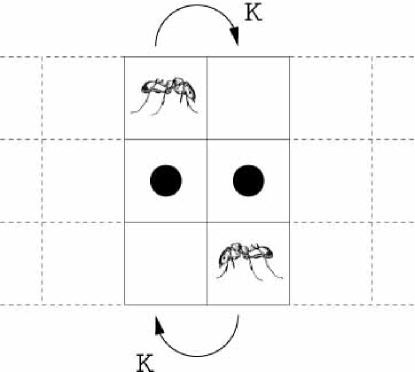
Figure 28: A typical head-on encounter of two oppositely moving ants in the model of bi-directional ant-traffic jscn ; the corresponding hopping probability is denoted by $K$. This process does not have any analog in the model of uni-directional ant-traffic.

a

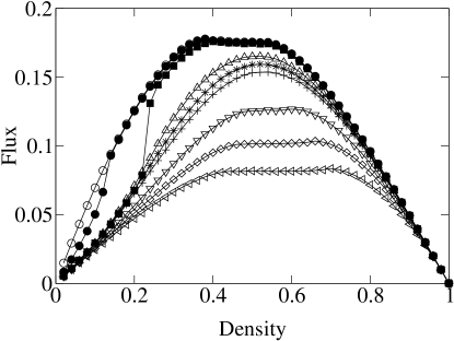
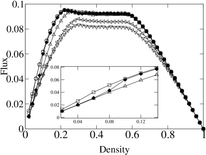
Figure 29: Fundamental diagrams of the model for bi-directional traffic jscn for the cases $q<K<Q$ (left) and $K<q<Q$ (right) for several different values of the pheromone evaporation probability $f$. The densities for both directions are identical and therefore only the graphs for one directions are shown. The parameters in the left graph are $Q=0.75,q=0.25$ and $K=0.5$. The symbols $\circ$, $\bullet$, $\blacksquare$, $\bigtriangleup$, $\ast$, $+$, $\bigtriangledown$, $\Diamond$ and $\triangleleft$ correspond, respectively, to $f=0,0.0005,0.005,0.05,0.075,0.10,0.25,0.5$ and $1$. The parameters in the right graph are $Q=0.75,q=0.50$ and $K=0.25$. The symbols $\circ$, $\square$, $\blacklozenge$, $\bigtriangleup$, $\triangleleft$ and $\bigtriangledown$ correspond, respectively, to $f=0,0.0005,0.005,0.05,0.5$ and $1$. The inset in the right graph is a magnified re-plot of the same data, over a narrow range of density, to emphasize the fact that the unusual trend of variation of flux with density in this case is similar to that observed in the case $q<K<Q$ (left). The lines are merely guides to the eye. In all cases curves plotted with filled symbols exhibit non-monotonic behaviour in the speed-density relation.

The rules governing the dropping and evaporation of pheromone in the model of bi-directional ant-traffic are identical to those in the model of uni-directional traffic. The common pheromone trail is created and reinforced by both the outbound and nestbound ants. The probabilities of forward movement of the ants in the model of bi-directional ant-traffic are also natural extensions of the similar situations in the uni-directional traffic. When an ant (in either of the two lanes) does not face any other ant approaching it from the opposite direction the likelihood of its forward movement onto the ant-free site immediately in front of it is $Q$ or $q$, respectively, depending on whether or not it finds pheromone ahead. Finally, if an ant finds another oncoming ant just in front of it, as shown in Fig. 28, it moves forward onto the next site with probability $K$. Since ants do not segregate in perfectly well defined lanes, head-on encounters of oppositely moving individuals occur quite often although the frequency of such encounters and the lane discipline varies from one species of ants to another. In reality, two ants approaching each other feel the hindrance, turn by a small angle to avoid head-on collision couzin and, eventually, pass each other. At first sight, it may appear that the ants in our model follow perfect lane discipline and, hence, unrealistic. However, that is not true. The violation of lane discipline and head-on encounters of oppositely moving ants is captured, effectively, in an indirect manner by assuming $K<Q$. But, a left-moving (right-moving) ant cannot overtake another left-moving (right-moving) ant immediately in front of it in the same lane. It is worth mentioning that even in the limit $K=Q$ the traffic dynamics on the two lanes would remain coupled because the pheromone dropped by the outbound ants also influence the nestbound ants and vice versa.

Fig. 29 shows fundamental diagrams for the two relevant cases $q<K<Q$ and $K<q<Q$ and different values of the evaporation probability $f$ for equal densities on both lanes. In both cases the unusual behaviour related to a non-monotonic variation of the average speed with density as in the uni-directional model can be observed jscn .

An additional feature of the fundamental diagram in the bi-directional ant-traffic model is the occurrence of a plateau region. This plateau formation is more pronounced in the case $K<q<Q$ than for $q<K<Q$ since they appear for all values of $f$. Similar plateaus have been observed earlier janowsky ; tripathy in models related to vehicular traffic where randomly placed bottlenecks slow down the traffic in certain locations along the route.

The experimental data available initially burd1 ; burd2 were not accurate enough to test the predictions mentioned above. However, more accurate recent data burd3 exhibit non-monotonic variation of the average speed with density thereby confirming our theoretical prediction.

One of the interesting open questions, which requires careful modelling, is as follows: how does a forager ant, which gets displaced from a trail, decides the correct direction on rejoining the trail? More specifically, an ant carrying food should be nest-bound when it rejoins the trail to save time and to minimize the risk of an encounter with a predator. In other words, do the pheromone trails have some “polarity” (analogous to the polarity of microtubules and actin, the filamentary tracks on which the cytoskeletal motors move)? On the basis of recent experimental observations, it has been claimed ratnieks1 that the trail geometry gives rise to an effective polarity of the ant trails. However, other mechanisms for polarity of the trails are also possible.

X Pedestrian traffic on trails

Although there are some superficial similarities between the trafic-like collective phenomena in ant-trails and the pedestrian traffic on trails, there are also some crucial differences. At present, there are very few models which can account for all the observed phenomena in completely satisfactory manner.

X.1 Collective phenomena

We present only a brief overview of the collective effects and self-organization; for a more comprehensive discussion, see ref.dhrev ; PedeProc .

Jamming: At large densities various kinds of jamming phenomena occur, e.g. when the flow is limited by a door or narrowing. Therefore, this kind of jamming does not depend strongly on the microscopic dynamics of the particles, but is typical for a bottleneck situation. It is important for practical applications, especially evacuation simulations. Furthermore, in addition to the flow reduction, effects like arching panic ; arching , known from granular materials, play an important role. Jamming also occurs where two groups of pedestrians mutually block each other.

Lane formation: In counterflow, i.e. two groups of people moving in opposite directions, a kind of spontaneous symmetry breaking occurs (see Fig. 30a). The motion of the pedestrians can self-organize in such a way that (dynamically varying) lanes are formed where people move in just one direction social . In this way, strong interactions with oncoming pedestrians are reduced and a higher walking speed is possible.

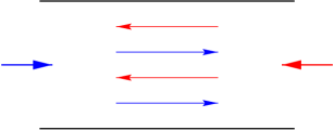
a)     b) 

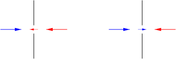
Figure 30: Patterns observed in counterflow. a) Lane formation in a narrow corridor. b) Oscillations of the flow direction at a door.

Oscillations: In counterflow at bottlenecks, e.g. doors, one can observe oscillatory changes of the direction of motion. Once a pedestrian is able to pass the bottleneck it becomes easier for others to follow in the same direction until somebody is able to pass (e.g. through a fluctuation) the bottleneck in the opposite direction (see Fig. 30b).

Patterns at intersections: At intersections various collective patterns of motion can be formed. Short-lived roundabouts make the motion more efficient since they allow for a “smoother” motion.

Panics: In panic situations, many counter-intuitive phenomena can occur. In the faster-is-slower effect panic a higher desired velocity leads to a slower movement of a large crowd. Understanding such effects is extremely important for evacuations in emergency situations.

X.2 Modelling Pedestrian Dynamics

Several different approaches for modelling the dynamics of pedestrians have been proposed, either based on a continuous representation of space or on a grid.

The earliest models of pedestrian dynamics belonged to the population-based approaches and took inspiration from hydrodynamics or gas-kinetic theory hydro ; hhydro ; hughes1 ; hughes2 . However, it turned our hhydro that several important differences to normal fluids are important, e.g. the anisotropy of interactions or the fact that pedestrians usually have an individual preferred direction of motion.

Later several individual-based approaches in continuous space and time have been proposed. In the social force models (see e.g. dhrev ; social and references therein) and other similar approaches TM95 pedestrians are treated as particles subject to repulsive forces induced by the social behaviour of the individuals. This leads to (coupled) equations of motion similar to Newtonian mechanics. There are, however, important differences since, e.g., in general the third law (“actio = reactio”) is not fulfilled. Furthermore a two-dimensional variant of the optimal-velocity model OV has also been suggested.

Active walker models activewalker ; trail have been used to describe the formation of human or animal trails etc. Here the walker leaves a trace by modifying the underground on his path. This modification is real in the sense that it could be measured in principle. For trail formation, vegetation is destroyed by the walker.

In chopard2 a kind of mesoscopic approach inspired by lattice gas models droz has been suggested. Thus the exclusion principle is relaxed and the dynamics is based on a collision-propagation scheme.

Most cellular automaton models for pedestrian dynamics proposed are rather simple fukui ; nagatani ; hubert and can be considered as two-dimensional generalizations of the ASEP (see Sec. III). However, these models are not able to reproduce all the collective effects described in the preceeding subsection. The same is true for more sophisticated discrete models gipps ; bolay .

In the following we discuss a promising new approach, the floor field model ourpaper ; ourpaper2 ; friction ; discrete , for the description of pedestrian dynamics in more detail which is takes inspiration from the ant trail model of Sec. IX. The interaction in this model is implemented as ’virtual chemotaxis’ which allows to translate a long-ranged spatial interaction into a local interaction with “memory”. Guided by the phenomenon of chemotaxis the interactions between pedestrians are thus local and allow for computational efficiency.

X.3 Floor field cellular automaton model

Pedestrians are modelled as particles that move on a two-dimensional lattice of cells. Each cell can be occupied by at most one particle which reflects that the interactions between them are repulsive for short distances (’private sphere’). Particles can move to one of the neighbouring cells based on certain transition probabilities that are are determined by three factors: (1) the desired direction of motion, (2) interactions with other pedestrians, and (3) interactions with the infrastructure (walls, doors, etc.).

First of all, basic transition probabilities are determined which reflect the preferred walking direction and speed of each individual in the form of a matrix of preferences $M$ which can be related to the preferred velocity vector and its fluctuations ourpaper .

Next interactions between pedestrians are taken into account. The exclusion principle accounts for the fact that one likes to keep a minimal distance from others. However, for larger distances the interaction is assumed to be attractive to capture the advantage in following the predecessor. This is implemented by virtual chemotaxis. Moving particles create a ”pheromone” at the cell which they leave, thus creating a kind of trace, the dynamic floor field $D$. It has its own dynamics given by diffusion and decay ourpaper which leads to a dilution and finally the vanishing of the trace after some time.

For a unified description another floor field is introduced, the static floor field $S$. It is constant and takes into account the interactions with the infrastructure, e.g. preferred areas, walls and other obstacles.

The transition probabilities given by the matrix of preference $M_{ij}$ are now modified by the strengths of the floor fields $D_{ij}$ and $S_{ij}$ in the target cell $(i,j)$; the details are given in ref.ourpaper . Due to the use of parallel dynamics it might happen that two (or more) pedestrians choose the same target cell. Such a situation is called a conflict. Due to hard-core exclusion, at most one persons can move. Introducing a friction parameter $\mu$ friction , with probability $\mu$ all pedestrians remain at their site, i.e. nobody is allowed to move. With probability $1-\mu$ one of the individuals is chosen randomly and allowed to move to the target cell. The effects of $\mu>0$ are similar to those arising from a moment of hesitation when people are about to collide and try to avoid the collision.

The details of the update rules can be found in ourpaper ; friction ; this floor field model has been able to reproduce the empirically observed phenomena listed earlier in this section. Another interesting phenomenon which has been studied successfully using the floor field model is the evacuation from a large space with only one exit ourpaper2 ; friction . However, this is beyond the scope of this review as we restrict our attention here mostly on traffic-like flow properties. Nevertheless the application of such models in the planning stages of large buildings, ships or aircrafts has become increasingly important over the last years. The simplicity and realism of the models allows to optimize evacuation and egress processes already in an early stage of the construction without the necessity of performing potentially dangerous experiments.

XI Summary and conclusion

Because of restrictions imposed by the allowed length of the review, we have excluded several biological traffic phenomena where, to our knowledge, very little progress has been made so far in theoretical modelling of the processes. These include, for example,
(i) bidirectional transport along microtubules where the same cargo moves along the same microtubule track using sets of opposing motors welte ; gross ;
(ii) self-organized patterns like, for example, asters and vortices, which have been in several in-vitro experiments nedlec and model calculations kardar ; sunil ; zimmer

In this article we have reviewed our current understanding of traffic-like collective phenomena in living systems starting from the smallest level of intra-cellular transport and ending at the largest level of traffic of pedestrians. So far as the theoretical methods are concerned, we have restricted our attention to those works where the language of cellular automata or extensions of TASEP has been used. The success of this modelling strategy has opened up a new horizon and, we hope, we have provided a glimpse of the exciting frontier.

Acknowledgements: It is our great pleasure to thank Yasushi Okada, Alexander John and Ambarish Kunwar for enjoyable collaborations on the topics discussed in this review. We are indebted to many colleagues for illuminating discussions although we are unable to mention all the names because of space limitations.

References

- (1) J. Howard, Mechanics of Motor Proteins and the Cytoskeleton, (Sinauer Associates, 2001) .
- (2) M. Schliwa (ed.), Molecular Motors, (Wiley-VCH, 2002).
- (3) D.D. Hackney and F. Tamanoi, The Enzymes, vol.XXIII, Energy Coupling and Molecular Motors (Elsevier, 2004).
- (4) M.K. Levin, in ref.schliwa .
- (5) D.J. Crampton and C.C. Richardson, in ref.hackney .
- (6) E.O. Wilson, The Insect Societies (Belknap, Cambridge, USA, 1971); B. Hölldobler and E.O. Wilson, The Ants (Belknap, Cambridge, USA, 1990)
- (7) H. Nagase and J. F. Woessner, J. Biol. Chem. 274, 21491 (1999).
- (8) M. Whittaker and A. Ayscough, Celltransmisions 17, 3 (2001).
- (9) W.T. Coffey, Yu. P. Kalmykov and J.T. Waldron, The Langevin Equation 2nd edn. (World Scientific, 2004).
- (10) H. Risken, The Fokker-Planck Equation, (Springer 1984).
- (11) A. Mogilner, L. Edelstein-Keshet, L. Bent and A. Spiros, J. Math. Biol. 47, 353 (2003).
- (12) S. Gueron, S.A. Levin and D.I. Rubenstein, J. Theor. Biol. 182, 85 (1996).
- (13) F. Schweitzer: Brownian Agents and Active Particles, Springer Series in Synergetics (Springer 2003).
- (14) E.M. Rauch, M. M. Millonas and D.R. Chialvo, Phys. Lett. A 207, 185 (1995).
- (15) S. Wolfram, Theory and Applications of Cellular Automata (World Sci., 1986); A New Kind of Science (Wolfram Research Inc., 2002)
- (16) B. Chopard and M. Droz, Cellular Automata Modeling of Physical Systems (Cambridge University Press, 1998).
- (17) J. Marro and R. Dickman, Nonequilibrium Phase Transitions in Lattice Models (Cambridge University Press, 1999).
- (18) V. Grimm, Ecological modeling, 115, 129 (1999); S. F. Railsback, Ecological modeling 139, 47 (2001); J. Odell, J. Object Technol. 1, 35 (2002); See also the special issue of the Proc. Natl. Acad. Sci. May 14, 2002, Supplement 3.
- (19) G.M. Schütz: Exactly Solvable Models for Many-Body Systems, in C. Domb and J.L. Lebowitz (eds.), Phase Transitions and Critical Phenomena, Vol. 19 (Academic Press, 2001).
- (20) D. Chowdhury, L. Santen, and A. Schadschneider, Phys. Rep. 329, 199 (2000); A. Schadschneider, Physica A 313, 153 (2002).
- (21) R. Mahnke, J. Kaupuzs and I. Lubashevsky, Phys. Rep. 408, 1 (2005).
- (22) M.R. Evans and R.A. Blythe, Physica A313, 110 (2002).
- (23) B. Derrida, M.R. Evans, V. Hakim and V. Pasquier, J. Phys. A 26, 1493 (1993).
- (24) G. Schütz and E. Domany, J. Stat. Phys.72, 277 (1993).
- (25) N. Rajewsky, L. Santen, A. Schadschneider and M. Schreckenberg, J. Stat. Phys. 92, 151 (1998).
- (26) M.R. Evans, N. Rajewsky and E.R. Speer, J. Stat. Phys. 95, 45 (1999).
- (27) J. de Gier and B. Nienhuis, Phys. Rev. E 59, 4899 (1999).
- (28) J. Krug, Phys. Rev. Lett. 67, 1882 (1991)
- (29) C. MacDonald, J. Gibbs, and A. Pipkin, Biopolymers 6, 1 (1968); C. MacDonald and J. Gibbs, Biopolymers 7, 707 (1969)
- (30) A.B. Kolomeisky, G. Schütz, E.B. Kolomeisky and J.P. Straley, J. Phys. A 31, 6911 (1998)
- (31) V. Popkov, L. Santen, A. Schadschneider and G.M. Schütz: J. Phys. A34, L45 (2001)
- (32) V. Popkov and G. Schütz, Europhys. Lett. 48, 257 (1999)
- (33) S.A. Janowsky and J.L. Lebowitz, Phys. Rev. A 45, 618 (1992)
- (34) G. Tripathi and M. Barma, Phys. Rev. Lett. 78 3039 (1997).
- (35) S. Goldstein and E.R. Speer, Phys. Rev. E 58, 4226 (1998).
- (36) J. Krug and P.A. Ferrari, J. Phys. A 29, L465 (1996).
- (37) M.R. Evans, Europhys. Lett. 36, 13 (1996); J. Phys. A 30, 5669 (1997).
- (38) D. Ktitarev, D. Chowdhury and D.E. Wolf, J. Phys. A 30, L221 (1997).
- (39) R. Juhasz, L. Santen and F. Igloi, Phys. Rev. Lett. 94, 10601 (2005), cond-mat/0507197.
- (40) A. Ebneth, R. Godemann, K. Stamer, S. Illenberger, B. Trinczek, E.M. Mandelkow and E. Mandelkow, J. Cell Biol. 143, 777 (1998).
- (41) K. Stamer, R. Vogel, E. Thies, E. Mandelkow and E.M. Mandelkow, J. Cell Biol. 156, 1051 (2002).
- (42) Y. Kafri, D.K. Lubensky and D. R. Nelson, Biophys. J. 86, 3373 (2004).
- (43) F. Jülicher, A. Ajdari, and J. Prost, Rev. Mod. Phys. 69, 1269 (1997).
- (44) P. Reimann, Phys. Rep. 361, 57-265 (2002).
- (45) R.P. Feynman, The Feynman Lectures on Physics, vol.1 (Addison-Wesley, 1963).
- (46) M. Smoluchowski, Physik. Z. 13, 1069 (1912).
- (47) T. Harms and R. Lipowsky, Phys. Rev. Lett. 79, 2895 (1997).
- (48) F. Marchesoni, Phys. Rev. E 56, 2492 (1997).
- (49) M.N. Popescu, C.M. Arizmendi, A.L. Salas-Brito and F. Family, Phys. Rev. Lett. 85, 3321 (2000).
- (50) L.B. Shaw, R.K.P. Zia and K.H. Lee, Phys. Rev. E 68, 021910 (2003).
- (51) L.B. Shaw, J. P. Sethna and K.H. Lee, Phys. Rev. E 70, 021901 (2004).
- (52) L.B. Shaw, A.B. Kolomeisky and K.H. Lee, J. Phys. A 37, 2105 (2004).
- (53) G. Lakatos and T. Chou, J. Phys. A 36, 2027 (2003).
- (54) T. Chou and G. Lakatos, Phys. Rev. Lett. 93, 198101 (2004).
- (55) G. Oster and H. Wang, in ref.schliwa .
- (56) M.E. Fisher and A.B. Kolomeisky, Proc. Natl. Acad. Sci. 98, 7748 (2001).
- (57) R.D. Astumian, Appl. Phys. A 75, 193 (2002).
- (58) M. Aridor and L.A. Hannan, Traffic 1, 836 (2000); 3, 781 (2002).
- (59) N. Hirokawa and R. Takemura, Trends in Biochem. Sci. 28, 558 (2003)
- (60) E. Mandelkow and E.M. Mandelkow, Trends in Cell Biol. 12, 585 (2002).
- (61) L.S. Goldstein, Proc. Natl. Acad. Sci. 98, 6999 (2001); Neuron 40, 415-425 (2003). 28, 558 (2003); Curr. Op. Neurobiol. 14, 564-573 (2004).
- (62) I. Derenyi and T. Vicsek, Phys. Rev. Lett. 75, 374 (1995).
- (63) I. Derenyi and A. Ajdari, Phys. Rev. E 54, R5 (1996).
- (64) Y. Aghababaie, G.I. Menon and M. Plischke, Phys. Rev. E 59, 2578 (1999).
- (65) R. Lipowksy, S. Klumpp, and Th. M. Nieuwenhuizen, Phys. Rev. Lett. 87, 108101 (2001).
- (66) Th. M. Nieuwenhuizen, S. Klumpp, and R. Lipowksy, Europhys. Lett. 58, 468 (2002).
- (67) S. Klumpp and R. Lipowksy, J. Stat. Phys. 113, 233 (2003).
- (68) S. Klumpp and R. Lipowksy, Europhys. Lett. 66, 90 (2004).
- (69) Th. M. Nieuwenhuizen, S. Klumpp, and R. Lipowksy, Phys. Rev. E 69, 061911 (2004).
- (70) S. Klumpp, Th. M. Nieuwenhuizen, and R. Lipowksy, Biophys. J. 88, 3118 (2005).
- (71) R. Lipowksy and S. Klumpp, Physica A 352, 53 (2005).
- (72) A. Parmeggiani, T. Franosch, and E. Frey, Phys. Rev. Lett. 90, 086601 (2003); Phys. Rev. E 70, 046101 (2004).
- (73) M.R. Evans, R. Juhasz, and L. Santen, Phys. Rev. E 68, 026117 (2003).
- (74) R. Juhasz and L. Santen, J. Phys. A 37, 3933 (2004).
- (75) V. Popkov, A. Rakos, R.D. Williams, A.B. Kolomeisky, and G.M. Schütz, Phys. Rev. E 67, 066117 (2003).
- (76) S. Mukherji and S.M. Bhattacharjee, J. Phys. A 38, L285 (2005).
- (77) B. Schmittmann and R.P.K. Zia, in C. Domb and J.L. Lebowitz (eds.), Phase Transitions and Critical Phenomena, Vol. 17 (Academic Press, 1995).
- (78) G.A. Klein, K. Kruse, G. Cuniberti and F. Jülicher, Phys Rev. Lett. 94, 108102 (2005).
- (79) K. Kruse and K. Sekimoto, Phys. Rev. E 66, 031904 (2002).
- (80) K. Nishinari, Y. Okada, A. Schadschneider and D. Chowdhury, Phys. Rev. Lett. 95, 118101 (2005).
- (81) Y. Okada and N. Hirokawa, Science 283, 1152 (1999).
- (82) Y. Okada and N. Hirokawa, Proc. Natl. Acad.Sci. USA 97, 640 (2000).
- (83) Y. Okada, H. Higuchi, and N. Hirokawa, Nature, 424, 574 (2003).
- (84) R. Nitta, M. Kikkawa, Y. Okada, and N. Hirokawa, Science 305, 678 (2003).
- (85) Y. Okada, K. Nishinari, D. Chowdhury, A. Schadschneider, and N. Hirokawa (to be published).
- (86) S. Saffarian, I. E. Collier, B.L. Marmer, E.L. Elson and G. Goldberg, Science 306, 108 (2004).
- (87) J. Mai, I.M. Sokolov and A. Blumen, Phys. Rev. E 64, 011102 (2001).
- (88) T. Antal and P.L. Krapivsky, cond-mat/0504652.
- (89) Y. Hiratsuka, M. Miyata and T. Q. P. Uyeda, Biochem. Biophys. Res. Commun. 331, 318 (2005).
- (90) A. Vartak et al. to be published.
- (91) D. B. Weibel, P. Garstecki, D. Ryan, W. R. DiLuzio, M. Mayer, J. E. Seto and G. M. Whitesides, Proc. Nat. Acad. Sci. USA, 102, 11963 (2005).
- (92) E. Bonabeau, G. Theraulaz, J.L. Deneubourg, S. Aron and S. Camazine, Trends in Ecol. Evol. 12, 188 (1997)
- (93) C. Anderson, G. Theraulaz and J.L. Deneubourg, Insect. Sociaux 49, 99 (2002)
- (94) Z. Huang and J.H. Fewell, Trends in Ecol. Evol. 17, 403 (2002).
- (95) E. Bonabeau, Ecosystems 1, 437 (1998).
- (96) G. Theraulaz, J. Gautrais, S. Camazine and J.L. Deneubourg, Phil. Trans. Roy. Soc. Lond. A 361, 1263 (2003).
- (97) J. Gautrais, G. Theraulaz, J.L. Deneubourg and C. Anderson, J. Theor. Biol. 215, 363 (2002).
- (98) L. Edelstein-Keshet, J. Math. Biol. 32, 303 (1994).
- (99) G. Theraulaz, E. Bonabeau, S.C. Nicolis, R.V. Sole, V. Fourcassie, S. Blanco, R. Fournier, J.L. Joly, P. Fernandez, A. Grimal, P. Dalle and J.L. Deneubourg, Proc. Natl.Acad. Sci. 99, 9645 (2002).
- (100) M. Dorigo, G. di Caro and L.M. Gambardella, Artificial Life 5(3), 137 (1999); Special issue of Future Generation Computer Systems dedicated to ant-algorithms (2000).
- (101) E. Bonabeau, M. Dorigo and G. Theraulaz, Nature 400, 39 (2000).
- (102) E. Bonabeau, M. Dorigo and G. Theraulaz, Swarm Intelligence: From Natural to Artificial Intelligence (Oxford University Press, 1999).
- (103) M.J.B. Krieger, J.B. Billeter and L. Keller, Nature 406, 992 (2000).
- (104) F.L.W. Ratnieks and C. Anderson, Insectes Sociaux 46, 95 (1999).
- (105) C. Anderson and F.L.W. Ratnieks, Am. Nat. 154, 521 (1999).
- (106) F.L.W. Ratnieks and C. Anderson, Am. Nat. 154, 536 (1999).
- (107) C. Anderson and F.L.W. Ratnieks, Insectes Sociaux 47, 198 (2000).
- (108) C. Anderson and D.W. McShea, Biol. Rev. 76, 211 (2001).
- (109) C. Anderson and F.L.W. Ratnieks, in: Complexity and complex systems in industry, eds. I.P. McCarthy and T. Rakotobe-Joel, (University of Warwick, U.K.), 92 (2000).
- (110) E. Bonabeau and C. Meyer, Harvard Business Review (May), 107 (2001).
- (111) S. Camazine, J.L. Deneubourg, N. R. Franks, J. Sneyd, G. Theraulaz, E. Bonabeau: Self-organization in Biological Systems (Princeton University Press, 2001).
- (112) A.S. Mikhailov and V. Calenbuhr, From Cells to Societies: Models of Complex Coherent Action (Springer, 2002).
- (113) J. Watmough and L. Edelstein-Keshet, J. Theor. Biol. 176, 357 (1995).
- (114) I.D. Couzin and N.R. Franks, Proc. Roy Soc. London B 270, 139 (2003).
- (115) D. Helbing, F. Schweitzer, J. Keltsch, P. Molnar: Phys. Rev. E56, 2527 (1997)
- (116) B. Derrida, Phys. Rep. 301, 65 (1998)
- (117) B. Derrida and M.R. Evans, in: Nonequilibrium Statistical Mechanics in One Dimension, ed. V. Privman (Cambridge University Press, 1997)
- (118) O.J. O’Loan, M.R. Evans, M.E. Cates, Europhys. Lett. 42, 137 (1998); Phys. Rev. E58, 1404 (1998).
- (119) D. Chowdhury, R.C. Desai, Eur. Phys. J. B15, 375 (2000)
- (120) A. Kunwar, D. Chowdhury, A. Schadschneider and K. Nishinari, submitted for publication.
- (121) M. Burd and N. Aranwela, Insect. Sociaux 50, 3 (2003).
- (122) D. Chowdhury, V. Guttal, K. Nishinari, A. Schadschneider, J. Phys. A:Math. Gen. 35, L573 (2002)
- (123) K. Nishinari, D. Chowdhury, A. Schadschneider, Phys. Rev. E 67, 036120 (2003)
- (124) P. F. Arndt, T. Heinzel and V. Rittenberg, J. Phys. A 31, L45 (1998); J. Stat. Phys. 97, 1 (1999).
- (125) N. Rajewsky, T. Sasamoto and E.R. Speer, Physica A 279, 123 (2000).
- (126) A. John, A. Schadschneider, D. Chowdhury and K. Nishinari, J. Theor. Biol. 231, 279 (2004).
- (127) M. Burd, D. Archer, N. Aranwela and D.J. Stradling, Am. Nat. 159, 283 (2002).
- (128) M. Burd et al. (2005) unpublished.
- (129) D. E. Jackson, M. Holcombe and F.L.W. Ratnieks, Nature, 432, 907 (2004).
- (130) D. Helbing: Rev. Mod. Phys. 73, 1067 (2001)
- (131) M. Schreckenberg, S.D. Sharma (Ed.): Pedestrian and Evacuation Dynamics, Springer 2001
- (132) D. Helbing, I. Farkas, T. Vicsek: Nature 407, 487 (2000)
- (133) D.E. Wolf and P. Grassberger (Editors): Friction, Arching, Contact Dynamics, (World Scientific, 1997)
- (134) D. Helbing, P. Molnar: Phys. Rev. E51, 4282 (1995)
- (135) L.F. Henderson: Transp. Res. 8, 509 (1974)
- (136) D. Helbing: Complex Systems 6, 391 (1992)
- (137) R. Hughes: Math. Comp. Simul. 53, 367 (2000)
- (138) R. Hughes: Transp. Res. B 36, 507 (2001)
- (139) P. Thompson and E. Marchant: Fire Safety Journal 24, 131 (1995)
- (140) A. Nakayama, K. Hasebe, Y. Sugiyama: Phys. Rev. E71, 036121 (2005)
- (141) D. Helbing, J. Keltsch, P. Molnar: Nature 388, 47 (1997)
- (142) S. Marconi, B. Chopard: In Cellular Automata, Lect. Notes Comp. Sc. 2493, 231 (2002)
- (143) B. Chopard, M. Droz: Cellular automata Modeling of Physical Systems, Cambridge University Press (1998)
- (144) M. Fukui and Y. Ishibashi: J. Phys. Soc. Jpn. 68, 2861 (1999)
- (145) M. Muramatsu and T. Nagatani: Physica A275, 281 (2000)
- (146) H. Klüpfel, T. Meyer-König, J. Wahle and M. Schreckenberg: in Theory and Practical Issues on Cellular Automata, S. Bandini, T. Worsch (Eds.), Springer (2000)
- (147) P.G. Gipps and B. Marksjös: Math. and Comp. in Simulation 27, 95 (1985)
- (148) K. Bolay: Diploma Thesis, Stuttgart University (1998)
- (149) C. Burstedde, K. Klauck, A. Schadschneider, J. Zittartz: Physica A295, 507 (2001)
- (150) A. Kirchner, A. Schadschneider: Physica A312, 260 (2002)
- (151) A. Kirchner, K. Nishinari, A. Schadschneider: Phys. Rev. E67, 056122 (2003)
- (152) A. Kirchner, H. Klüpfel, K. Nishinari, A. Schadschneider, M. Schreckenberg: J. Stat. Mech.: Theor. Exp., P10011 (2004)
- (153) M.A. Welte, Curr. Biol. 14, R525 (2004).
- (154) S.P. Gross, Phys. Biol. 1, R1 (2004).
- (155) F.J. Nedlec, T. Surrey, A.C. maggs and S. Leibler, Nature 389, 305 (1997); T. Surrey, F. Nedlec, S. Leibler and E. Karsenti, Science 292, 1167 (2001); F. Nedlec, T. Surrey and E. Karsenti, Curr. Op. Cell Biol. 15, 118 (2003).
- (156) H. Y. Lee and M. Kardar, Phys. Rev. E 64, 056113 (2001).
- (157) S. Sankararaman, G. I. Menon and P.B. Sunil Kumar, Phys. Rev. E 70, 031905 (2004).
- (158) F. Ziebert and W. Zimmermann, cond-mat/0502236 (2005).