physics/0509016

CARE/ELAN Document-2005-013

CLIC Note 639

KEK Preprint 2005-60

LAL 05-94

September 2, 2005

Conceptual Design of a Polarised Positron Source Based on Laser Compton Scattering
— A Proposal Submitted to Snowmass 2005 —

Sakae Araki, Yasuo Higashi, Yousuke Honda, Yoshimasa Kurihara, Masao Kuriki,

Toshiyuki Okugi, Tsunehiko Omori, Takashi Taniguchi, Nobuhiro Terunuma, Junji Urakawa

(KEK, Ibaraki, Japan)

X. Artru, M. Chevallier

(IPN, Lyon, France)

V. Strakhovenko

(BINP, Novosibirsk, Russia)

Eugene Bulyak, Peter Gladkikh

(NSC KIPT, Kharkov, Ukraine)

Klaus Mönig

(DESY, Zeuthen, Germany & LAL, Orsay, France)

Robert Chehab, Alessandro Variola, Fabian Zomer

(LAL, Orsay, France)

Susanna Guiducci, Pantaleo Raimondi

(INFN, Frascati, Italy)

Frank Zimmermann

(CERN, Geneva, Switzerland)

Kazuyuki Sakaue, Tachishige Hirose, Masakazu Washio

(Waseda University, Tokyo, Japan)

Noboru Sasao, Hirokazu Yokoyama

(Kyoto University, Kyoto, Japan)

Masafumi Fukuda, Koichiro Hirano, Mikio Takano

(NIRS, Chiba, Japan)

Tohru Takahashi, Hiroki Sato

(Hiroshima University, Hiroshima, Japan)

Akira Tsunemi

(Sumitomo Heavy Industries Ltd., Tokyo, Japan)

Jie Gao

(IHEP, Beijing, China)

Viktor Soskov

(IHEP, P.N. Lebedev Physical Institute, Russian Academy of Sciences, Moscow)

Abstract

We describe a scheme for producing polarised positrons at the ILC from polarised X-rays created by Compton scattering of a few-GeV electron beam off a ${\rm CO}_{2}$ or YAG laser. This scheme is very energy effective using high finesse laser cavities in conjunction with an electron storage ring.

1 Introduction

 

At the ILC there exists a well motivated physics case to have not only the electron beam, but also the positron beam polarised [1]. Up to now two ideas to produce polarised positrons have been studied in detail. Both schemes first produce polarised photons which are then converted into polarised positrons in a thin target. In the first scheme the polarised positrons are produced in a helical undulator by the high energy electron beam upstream of the interaction point [2]. In the second scheme the photons are produced by Compton scattering of a 6 GeV electron beam off a ${\rm CO}_{2}$ laser [3].

The undulator scheme seems technically easier. However it requires the electron linac to be fully operational before positrons can be produced and it adds an additional energy spread of 0.15% to the electron beam. Also some important problems like the vacuum in the undulator and radiation on the beampipe inside the undulator still need to be solved. For the Compton scattering solution a high current electron beam needs to be produced and a complicated high power laser scheme is needed. However the positron polarisation can be switched easily by switching the laser polarisation and the reachable degree of polarisation is in principle higher than for the undulator scheme.

In this note some ideas are presented on how the time structure of the ILC could be utilised to produce polarised positrons by Compton scattering of an electron beam in a storage ring and a laser resonator. R&D for technical improvements toward an high finesse resonator (Gain$>10000$, see appendix A) would obviuosly strongly reduce the cost and the complexity of the proposed design.

This note is meant as a basis for first discussions with accelerator experts to understand if this scheme is possible at all.

1.1 Basics of Compton scattering

The kinematics and cross section of Compton scattering is governed by the variable

$$x=\frac{4E_{b}\omega_{0}}{m^{2}c^{4}}\cos^{2}{\frac{\alpha}{2}}\simeq 0.019\left[\frac{E_{b}}{{\,\mathrm{Ge\kern-1.00006ptV}}}\right]\left[\frac{\mu m}{\lambda}\right],$$

representing the scaled squared centre of mass energy of the electron-photon system. $E_{b}$ denotes the electron beam energy and $\omega_{0}$ the energy of the laser photons. $\alpha$ is the crossing angle of the electron beam and the laser. The maximum energy of the scattered photons is given by $E_{\gamma}<x/(x+1)E_{b}$. Relevant $x$ values for polarised positron production are $x={\cal O}(0.01)$.

Since Compton scattering conserves parity, the total and differential cross section cannot depend on the individual electron and laser polarisations, but only on their product ${\cal P}_{e}\lambda_{\gamma}$.

Figure 1 shows the total cross section as a function of $x$ and the photon energy spectrum for $x=0.01$ for ${\cal P}_{e}\lambda_{\gamma}=0$ and ${\cal P}_{e}\lambda_{\gamma}=-1$. The $x$ dependence of the cross section in the relevant range is small and the polarisation dependence almost negligible. The photon spectrum shows two peaks at zero and at maximum energy.

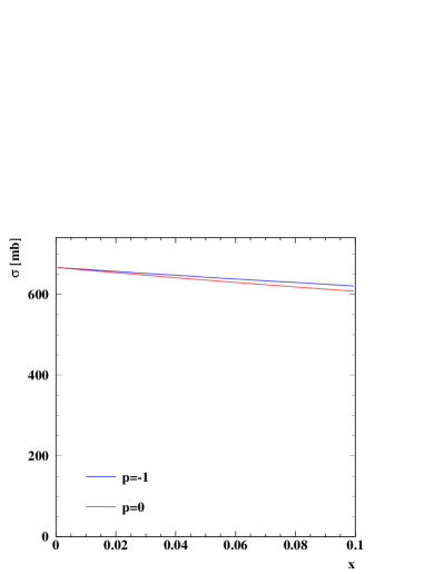
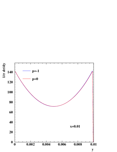
Figure 1: Total Compton cross section (left) and photon energy spectrum (right) for different electron/laser polarisation. P denotes the product of the two polarisations, y denotes the photon energy scaled to the beam energy.

The scattered photon polarisation depends on the laser and electron polarisation separately and is shown in figure 2 as a function of the photon energy for ${\cal P}_{e}\lambda_{\gamma}=-1$ The dependence on the electron polarisation is very small at small $x$ so that there is no need for electron polarisation in the storage ring. For a highly polarised laser very high $\gamma$ polarisation can be achieved at high energy. Since also the polarisation transfer to the positron in the pair production works best at high energy transfer the high energy positrons will be highly polarised.

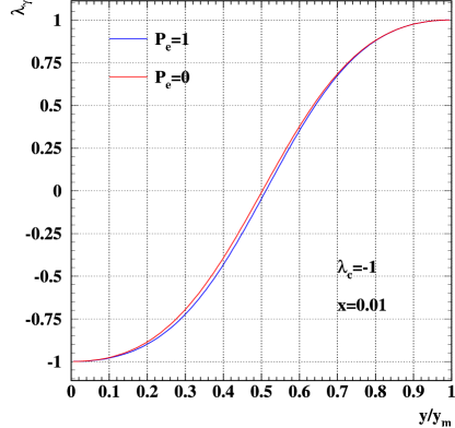
Figure 2: Photo polarisation as a function of $x$ for 100% laser polarisation and different electron polarisations

1.2 The laser cavity scheme

In the damping ring the $e^{+}$ are stored with a much smaller distance than in the main accelerator. In this note it will be assumed that a distance of 3 ns is possible. This bunch spacing can also be used for the positron production. It might thus be possible to store the electrons for the Compton scattering in a storage ring with 1 m bunch spacing and collide them in one or few points with a laser cavity. The length of this storage ring is arbitrary too a large extent. The photons are converted into positrons in a thin target and the positrons are captured in the same way as in the other schemes. The positrons are then accumulated in the damping ring or in a special accumulator ring. If it is technically possible accumulation in the damping ring saves the cost of the extra accumulator ring. However in this case the time between two trains needs to be shared between positron accumulation and damping. A sketch of the proposed scheme is shown in figure 3. If the full time can be used for positron generation each bunch can receive positrons from about 20000 beam-laser interactions.

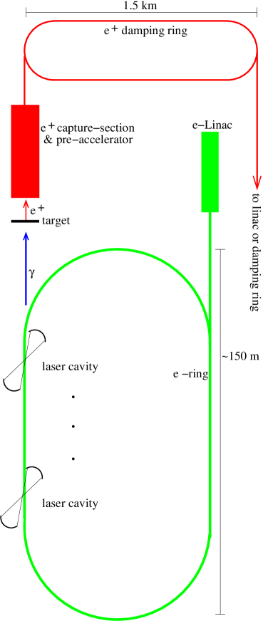
Figure 3: Principle scheme of the proposed system

For the laser cavity two concepts will presented, wither a solid state laser, like Nd:Yag with a wavelength of $\lambda=1.06\mu\mathrm{m}$ or a ${\rm CO}_{2}$ laser with a wavelength of $\lambda=10.6\mu\mathrm{m}$. For identical laser parameters the ${\rm CO}_{2}$ has ten times more photons/pulse than the Nd:Yag, however in practice the Nd:Yag laser can be focused to a significantly smaller spot size. Furthermore the Nd:Yag laser technology is better suited to develop high finesse resonators to improve the photon intensity. Also the Compton ring energy needs to be higher in the ${\rm CO}_{2}$ version to obtain the same scattered photon energy.

2 Compton Ring Design and Simulation of Compton Scattering

 

2.1 Necessary frame parameters

Necessary frame parameters of the Compton Rings (CR) are given and listed in Table 1. CR should be capable to emit $1.39\times 10^{10}$ gamma-quanta within the energy range $23.2\ldots 29$ MeV per bunch passed through the interaction section.

Table 1: List of parameters of Compton rings

parameter	CO2	YAG
Electron energy (GeV)	4.1	1.3
Electron bunch charge (nC)	10	10
RF frequency (MHz)	650	650
Hor beam size at IP, rms ($\mu$m)	25	25
Ver beam size at IP, rms ($\mu$m)	5	5
Bunch length at IP, rms (mm)	5	5
Laser photon energy (eV)	0.116	1.164
Laser radius at IP, rms ($\mu$m )	25	5
Laser pulse width, rms (mm)	0.9	0.9
Laser pulse power / cavity (mJ)	210	592
Number of laser cavities (IPs)	30	30
Crossing angle (degrees)	8	8

Remarks to the table:

The transverse bunch dimensions at the interaction points (IPs) are consistent with the horizontal emittance $0.5$ nm rad, the coupling $0.02$, and $\beta_{x,z}$–function values $1.25$ m and $2.5$ m, respectively. The bunch length is not directly employed in the calculations.

2.2 Brief review of laser–electron interactions

To estimate feasibility of Compton ring, here a brief classification of photon–electron interaction is presented.

Electron–photon interactions mainly governed by two parameters: (i) the density of photons (field strength in classical electrodynamics), and (ii) the energy of each laser photon (frequency in classical electrodynamics). We will refer to the first parameter as the parameter of nonlinearity, to the second as the quantumness (essentially quantum description of the process).

For the Compton ring it is expedient to present the parameter of nonlinearity (see [4, 5]) as

$$\xi^{2}=2\lambdabar_{\mathrm{C}}r_{0}\lambda N=\frac{3}{4\alpha\pi}\sigma_{\mathrm{C}}\lambda_{\mathrm{las}}N_{\mathrm{las}}\approx 32.7\times N_{X}\;.$$ (1)

Here $\alpha$ is the fine-structure constant, $r_{0}$ the classical electron radius, $N_{X}$ number of gammas scattered by each electron in the bunch when travelling over a wavelength of laser radiation.

Thus, the radiation begins to transform into the synchrotron spectrum if the electron scatters more than 3 quanta per 100 laser wavelengths.The linear Compton (Thomson) scattering takes place when $\xi^{2}\ll 1$.

Quantum effects – recoil of the electron when scattering off the laser photon which lead to change the cross section and spectrum – are governed by the parameter

$$a=2(1+\cos\varphi)\frac{\gamma E_{\mathrm{las}}}{m_{e}c^{2}}=\frac{E_{X}^{\mathrm{max}}}{E_{\mathrm{beam}}}\;.$$ (2)

If $a\ll 1$ then no quantum effects such as decreasing of the cross section and of the energy of scattered gamma-ray quantum are appeared.

2.3 Estimations

Generation of the required amount of gamma–ray quanta imposes certain demands upon number of laser photons scattered off the electron per a passage through all 30 IPs (IPs section): Each of $6.24\times 10^{10}$ should in average scatter off $0.223$ of gamma–ray quanta with the energy within $23.2\ldots 29$ MeV interval. Since the total length of all IPs is $30\times 0.9\times 2.5=67.7$ mm $\approx 6770$ wavelengths of CO2 laser $\lambda\approx 10\,\mu$m, then the condition of linear Compton scattering fulfils. For the case considered – $E_{X}=29$ MeV, $E_{\mathrm{beam}}=4.1$ GeV – the parameter $a\approx 10^{-2}\ll 1$. Thus, the conditions for the linear Compton (see, e.g., Thomson [6]) are fully satisfied.

For the linear Compton spectrum, within the energy interval of $23.2\ldots 29$ MeV there emitted are $0.248$ of the total number of photons. The required number of photons is bigger than estimated above, about $0.9$ of gammas per electron’s passage through IPs section. Nevertheless, the conditions for linear Compton scattering are still satisfied with good margins.

The spectrum of collimated gamma rays in small-angle approximation (see [7]) is presented in Fig.4. The collimator was adjusted to cut out gammas with energy below $23.2$ for the ideal case of parallel electron trajectories and zero energy spread.

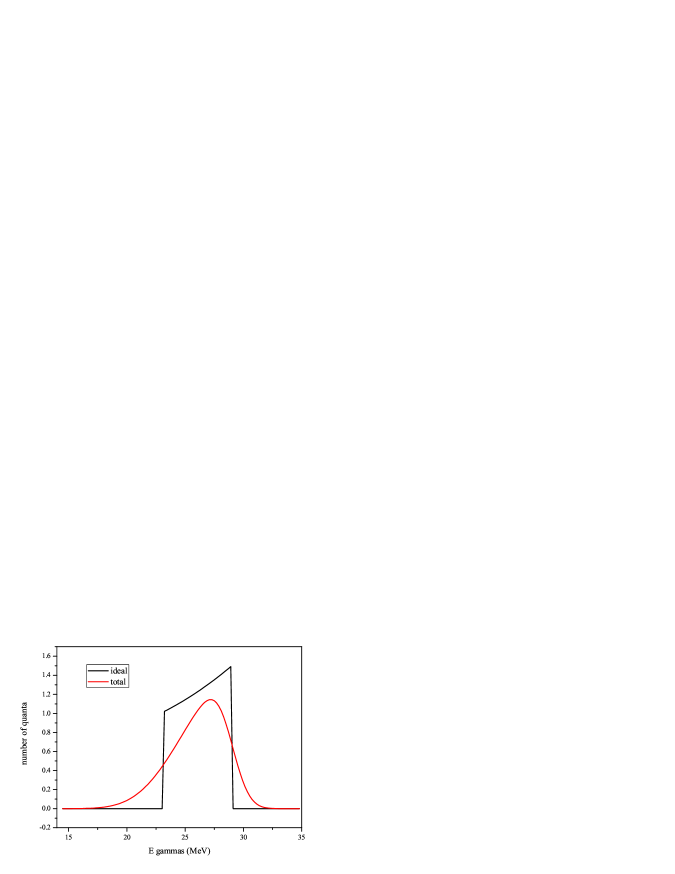
Figure 4: Collimated spectra of gammas. Black curve for the ideal case, red for simulated

2.4 Compton ring dynamics

Statistical properties of the bunches circulating in Compton storage rings are mainly governed by the synchrotron radiation and scattering of laser photons off the electrons.

Being statistically independent, these two processes establish the stationary properties of the bunches – emittances, squared energy spread $s^{2}$, or squared bunch length $\sigma_{y}^{2}$ – as (see [8])

$$s^{2}=\frac{s_{s}^{2}\Delta E_{s}+s_{X}^{2}\Delta E_{X}}{\Delta E_{s}+\Delta E_{X}}\;,$$ (3)

where $s_{X}=\left.\Delta E_{\mathrm{beam}}\right/E_{\mathrm{beam}}$ is the partial Compton energy spread (rms).

The squared partial Compton energy spread and rms bunch length read

$$s_{x}^{2} = \frac{E_{X}^{\mathrm{max}}}{6E_{\mathrm{beam}}}\;;$$ (4)

$$\sigma_{y}^{2} = \frac{\alpha_{1}E_{X}^{\mathrm{max}}hw^{2}}{12\pi eV_{\mathrm{rf}}}\;,$$ (5)

with $w\equiv c\left/f_{\mathrm{rf}}\right.$ being the width of rf bucket (for 650 MHz $w=0.461$ m), $\alpha_{1}$ the linear momentum compaction factor. As it should be emphasised, the partial Compton energy spread for a given spectrum is determined only by the energy of circulating electrons.

Energy loss of the electron for the rings under consideration is $\Delta E_{X}=0.9\times 29/2=11.2$ MeV per passage (or turn).

Synchrotron losses depend on the radius of curvature $\rho$ in the bending magnets and the energy of electrons. The radius of curvature is

$$\rho=\frac{E_{\mathrm{beam}}}{0.3B}$$

where $\rho$ in meters, $B$ is the dipole field strength in Tesla, $E_{\mathrm{beam}}$ the energy of electrons in GeV. Energy losses $\Delta E$ (in keV) per turn is

$$\Delta E_{s}=\frac{88.5E^{4}}{\rho}=26.55BE_{\mathrm{beam}}^{3}\,.$$

Hence, for $E_{\mathrm{beam}}=4.1$ GeV and $B=0.63377$ Tesla every electron looses $1.160$ MeV/turn which is sufficiently smaller as compared with the Compton losses ($11.2$ MeV/turn, see above). The beam dynamics in CO2 ring will be laser-dominated, the rms steady–state energy spread (4) $\left.\Delta E_{\mathrm{beam}}\right/E_{\mathrm{beam}}=3.43\times 10^{-2}$. Hence, to provide stable lossless circulation of the beam, a low–compaction optics is almost mandatory [9].

For the listed in Table 1 parameters and the extremely low compaction optics (see [10]), $\alpha_{1}=2\times 10^{-6}$, the partial Compton stationary bunch length is $4.85$ mm. Computation of steady–state yield for CO2 ring with $\alpha_{1}=2\times 10^{-6}$ and other parameters from Table 1 by an analytical code based on (3) for all three degrees of freedom results in following: the yield per electron passage through IPs is $0.43$, the bunch length $4.53$ mm, the horizontal emittance reduced down to $8.64\times 10^{-11}$ rad m. Thus, number of $(23.2\dots 29)$ MeV gammas is $6.2346\times 10^{9}$.

Summarising the feature of steady–state regime of Compton ring operation, it has to be stated that this regime is unacceptable due to the following reasons:

1. very high RF voltage is required to provide stable motion: if average energy losses per turn exceeds RF amplitude, the RF bucket vanishes, see eq. (6) for $q\leq 1$;

2. even if RF voltage is high enough, fluctuations in number and energy of emitted gammas results in very short beam life time (i.e. high quantum losses);

3. and even the short life time could be regarded as tolerable, bunch lengthening up to the steady–state will reduce the gamma yield below demands.

2.5 Pulsed mode: basic idea

Consider a ring with very low synchrotron number $Q_{s}$ such that the inverse to it – the period of synchrotron oscillations – much exceeds the temporal length of gamma burst $T_{X}$: $T_{X}\ll 1/Q_{s}$. Under such condition we can consider the bunch as free, moving in the phase plane straight with constant velocity. (Transformation of the energy spread into the bunch length takes at least a quarter of the synchrotron period.) Interactions of the bunch with the laser pulse (recoils) result in Brownian dispersion and offset along the momentum axis $p$ (here and below $p$ is relative deviation of the energy of electron $E_{e}$ from the synchronous $p\equiv(E_{e}-E_{\mathrm{beam}})/E_{\mathrm{beam}}$): The dispersion and offset after $n$–th turn are $\sigma_{p}^{2}(n)=n\left<\Delta p^{2}\right>$ and $S_{\mathrm{dr}}=n\left<\Delta p\right>$, respectively. The offset is caused by drift due to the fact that any interaction of the electron with a laser pulse results decreasing $p$.

Thus, if we set a bunch at the location in the phase space where the phase velocity directs vertically (along $p$–axis) and is equal to the drift velocity opposite to it, then the bunch during the burst will not change location of its centre-of-weight and length.

The scheme will be improved if the curvature of phase trajectories at the initial bunch location is low, which can be attained for the nonlinear ring optics with sufficient cubic term in the phase slip factor.

2.6 Simulations

Simulations were performed with a code intended for modelling the longitudinal dynamics in Compton rings with nonlinear compaction [11]. The code represents a turn constructed from 4 sections:

1. IPs – a particle can experience a series of random kicks, probability of which conforms with the particle phase coordinate $\phi$ and 3-D Gaussian distributed photon population in laser pulse; the random amplitude of the kick obeys the linear Compton spectrum.

2. SL – losses due to synchrotron radiation: every particle experiences the regular kick with amplitude proportional to the particle instant energy $p$.

3. DRIFT – the phase of the particle advances as $\phi_{f}=\phi_{i}+\kappa_{1}p+\kappa_{2}p^{2}+\kappa_{3}p^{3}$ ($\kappa_{j}$ are the normalised phase slip factors).

4. RF – zero–length harmonic rf cavity: every particle receives a kick with amplitude depending of its phase, $p_{f}=p_{i}-U_{\mathrm{rf}}\sin\phi$.

5. STAT – in–flight statistics of the bunch.

The particle in the bunch is represented by the flat zero–length disk with 2-Dim density distribution.

First simulations were performed to validate basic idea of the pulsed mode. The simulations have proved our expectations true.

Then simulations of the both CO2 and YAG rings were performed. For each of the rings two optics were chosen: a conventional linear (‘lin’) and a low–alpha nonlinear (‘nl’) with compaction factors like [10]. The quadratic compaction factors, $\alpha_{2}$, were chosen to provide zero value to the quadratic phase slip factors $\kappa_{2}$, see [12]. For every optics, the initial position of the bunch in the phase plane were being set manually to attain about a maximal average yield over the given number of turns.

Results are summarised in Table 2.

Table 2: Results of simulations

parameter	CO2 con	CO2 nl	YAG con	YAG nl
Linear comp $\alpha_{1}$	$1\times 10^{-4}$	$2\times 10^{-6}$	$1\times 10^{-4}$	$2\times 10^{-6}$
NL comp $\alpha_{2}$	$-2\times 10^{-4}$	$-4\times 10^{-6}$	$-2\times 10^{-4}$	$-4\times 10^{-6}$
NL comp $\alpha_{3}$	$0$	$2\times 10^{-3}$	$0$	$2\times 10^{-3}$
RF voltage ( MV )	20	20	20	20
Harmonic number	$1408$	$1408$	$600$	$600$
Turns laser on	$50$	$50$	$100$	$100$
Aver. gammas/electron	$0.39$	$1.24$	$0.21$	$0.94$
[23.2-29] MeV gam/pulse	$5.65\times 10^{9}$	$1.78\times 10^{10}$	$3.0\times 10^{9}$	$1.36\times 10^{10}$

There were not lost particles for the both rings in $4500$-turns operating cycle with the first 50 or 100 turns with the laser on.

It should be pointed out that the maximal theoretical yields for the given geometry – the crossing angle, transversal dimensions of the bunch and all dimensions of the laser pulse are $2.78\times 10^{10}$ (CO2) and $3.04\times 10^{10}$ (YAG).

Number of scattered quanta per electron per passage through IP obtained from simulations is presented in Fig.5.

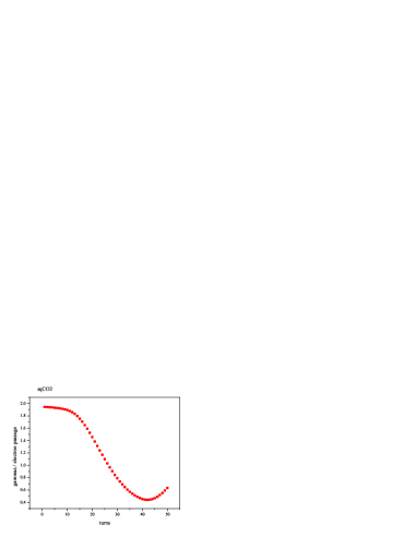
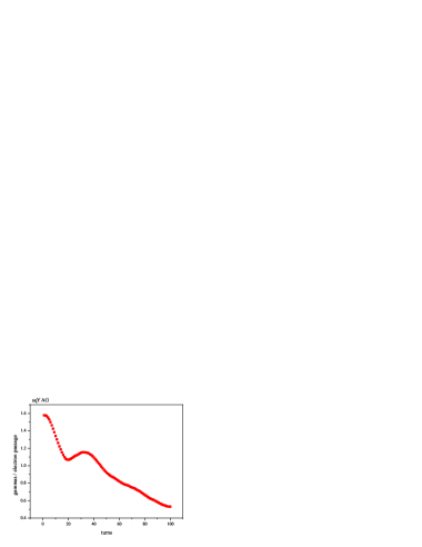
Figure 5: Yield vs turn, nonlinear rings. Left – CO2, right – YAG

Nonlinear dependence of the yield on time occurs due to deviation of the bunch centre of weight, as presented in Fig.6.

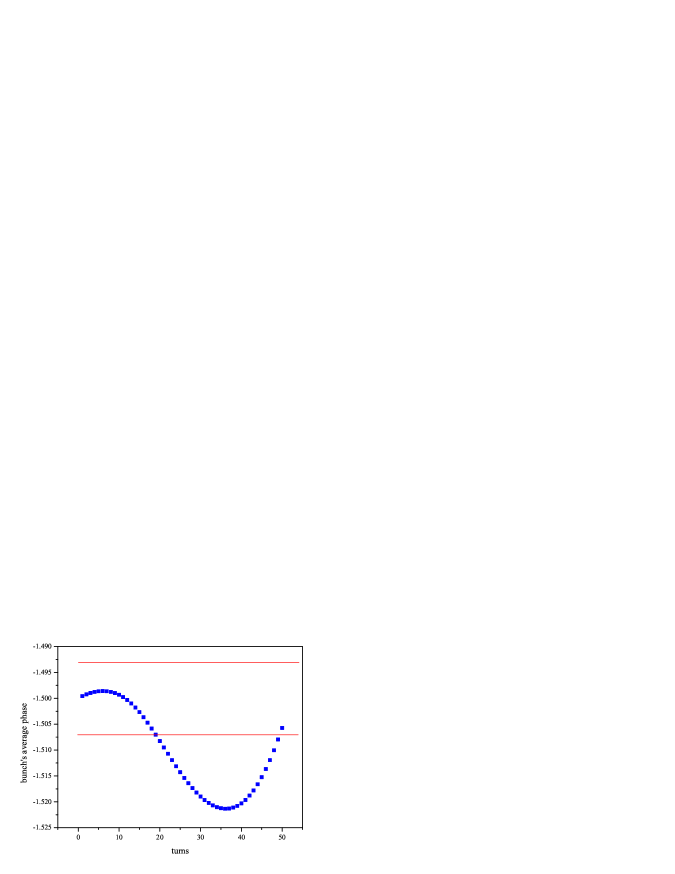
Figure 6: Centre-of-weight excursion. Band with red border lines represent effective rms interaction length

As it can be seen, the minimum in yield caused by the bunch offset from the laser focus.

In Fig.7 there presented is distribution of electrons over the phase space in YAG NL ring after 100 turns. The vertical red line indicates the phase position of the laser pulse.

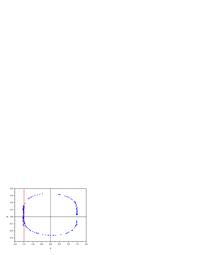
Figure 7: Phase distribution of electrons in the bunch after 100 turns

2.7 Conclusion

The considered systems in the pulsed mode are capable to meet demands imposed upon the Compton ring with good margins for the stored laser power and the bunch density. It seems that fine adjustment of the parameters, especially the ring nonlinearity, initial bunch position in the phase plane, and laser-to-bunch matching, can enhance the system performance.

3 Beam Stacking in Damping Ring

 

The ideal choice of accumulation ring turns out to be the damping ring itself. Due to its large circumference, it can store the full number of positron bunches, while at the same time providing a significant damping over the 10 ms repetition period of the laser-beam collisions in the Compton ring. In addition, the longitudinal bucket areas of the proposed damping rings is large (due to the small momentum compaction factor and high rf voltage), which facilitates stacking. Choosing the damping ring for accumulation also avoids constructing another ring. The damping ring will accumulate for 100 ms and then damp for another 100 ms (close to 10 damping times), for a main-linac repetition rate of 5 Hz.

The damping ring should store 2800 bunches with a bunch spacing of about 3.077 ns (325 MHz). The corresponding ring circumference is about 3.3 km. The beam energy in the damping ring is chosen as 5 GeV. The beam in the ring consists of 10 trains, each with 280 bunches. The longitudinal damping time is about 10 ms.

Each injected positron bunch coming from the laser-Compton ring has a bunch population of $2.4x10^{8}$. Injection occurs into all 2800 buckets on 10 consecutive turns. This 10-turn injection is followed by a 20-ms of damping, after which the next 10-turn injection starts. The whole process of injection and damping repeats 10 times. After 10 injections, the bunch charge is about $2.4\times 10^{10}$ positrons.

The transverse rms emittance of the injected positrons is of order 0.0015 rad-m for an undulator source and 0.006-0.007 rad-m for a conventional source [13]. We expect similar values for a source based on Compton back scattering. The “edge emittance” and, therefore, the required acceptance is about 10 times larger than the rms emittance [13]. The rms energy spread of the injected beam at 5 GeV is taken to be of order 0.14% and the rms bunch length 3 mm. The injected energy spread is close to the equilibrium value, the bunch length is about two time shorter.

The rf frequency of the damping ring is taken as 650 MHz. then the length of the rf bucket is about 45 cm, about 15 times the injected bunch length of 3 mm. Therefore, it should be possible to inject 10 bunches into the bucket without damping. For a more precise estimate, it is instructive to compute the bucket area.

The maximum energy deviation at the centre of the rf bucket is

$$\left(\frac{\Delta p}{p_{0}}\right)_{\rm max}^{2}=\frac{eV_{\rm rf}\sin\psi_{s}}{\pi h|\eta_{c}|cp_{0}}2\left(\sqrt{q^{2}-1}-{\rm arccos}\frac{1}{q}\right)\;,$$ (6)

where $q=eV_{\rm rf}/U_{0}$ is the peak energy gain from the rf system divided by the energy loss per turn, and

$$\psi_{s}={\rm arccos}\left(\frac{U_{0}}{eV_{\rm rf}}\right)\;$$ (7)

the synchronous phase angle.

The full length of the bucket is given by

$$l_{\rm bucket}=\frac{\lambda_{rf}}{2\pi}(\psi_{1}-\psi_{2})\;,$$ (8)

with $\psi_{1}$ and $\psi_{2}$ denoting two solutions of the transcendent equation

$$\cos\psi_{1,2}+\psi_{1,2}\sin\psi_{s}=(\pi-\psi_{s})\sin\psi_{s}-\cos\psi_{s}\;.$$ (9)

One of the two solutions is $\psi_{1}=\pi-\psi_{s}$. The second solution $\psi_{2}$ has to be determined numerically.

The total bucket area is estimated as

$$A_{\rm bucket}\approx\pi\;(\Delta E_{\rm max})\;(\Delta t)_{\rm max}$$ (10)

where $\Delta E_{\rm max}\approx c\;\Delta p_{\rm max}$ is the maximum energy deviation at the centre of the bucket, and $(\Delta t)_{\rm max}=l_{\rm bucket}/(2c)$, the bucket half length in units of seconds.

Table 3: Example parameters of damping ring employed for positron stacking.

energy	5 GeV
circumference	3323 m
particles per extracted bunch	$2.4\times 10^{10}$
rf frequency	650 MHz
number of trains	10
number of bunches per train	280
gap between trains (no. of missing bunches)	80
particles per injected bunch	$2.4\times 10^{8}$
injections per bucket on successive turns	10
injection repetition rate during 100 ms	100 Hz
total number of injections	100
store time after 100 injections	100 ms
energy loss per turn	5.5 MeV
damping time	10 ms
transverse emittance at injection	0.005 rad-m
rms bunch length at injection	3 mm
rms energy spread at injection	0.14%
final rms bunch length	6 mm
final rms energy spread	0.14%
longitudinal “edge” emittance at injection	0.7 meV-s
rf voltage	20 MV
momentum compaction	$3\times 10^{-4}$
2nd order momentum compaction	$1.3\times 10^{-3}$
synchrotron tune	0.0365
bucket area	292 meV-s
synchronous phase	15.58∘
separatrix phases 1 & 2	$164.42^{\circ}$, $-159.19^{\circ}$
maximum momentum acceptance	$\pm 2.7$%

We have simulated the efficiency of the stacking process. The simulation considers only the longitudinal phase space. It includes a sinusoidal rf voltage, and the first and second order momentum compaction factors. Radiation damping and quantum excitation are modelled as in [14]. Damping-ring and beam parameters assumed for this simulation are listed in Table 3. They are similar to those of the 3-km ILC damping ring designs PPA and OTW [15].

The injection septum is placed at a location with large dispersion, since the stacking is performed in longitudinal phase space. The septum blade is assumed to be small compared with the transverse dispersive beam size. Between successive turns of injection, the orbit at the septum is varied with fast bumper magnets. It may prove necessary to install injection septa on either side of the beam pipe, and to move the orbit from one side to the other after 5 from 10 injections, so as to facilitate the injection of bunches with opposite sign of relative momentum deviation and optimum phase-space coverage over 10 turns.

The energy of the injected beam is ramped such that the transverse position of the septum always corresponds to a separation of $2\sigma_{\delta}$ from the beam centroid, taking into account the local dispersion value. Consequently, positrons of the stored beam being closer than $2\sigma_{\delta}$ to the injected beam at the turn of injection are considered lost. Likewise, injected positrons with a momentum offset of more than $2\sigma_{\delta}$ from the injected beam centroid energy, in the direction towards the bucket centre, are also taken to be lost. The initial energy offset is first changed from $-1.05$% to $-2.45\%$, in steps of $-0.35\%$ from turn to turn, and then from $+1.05$% to $+2.45\%$ in steps of $+0.35\%$, over a total number of 10 turns. The point $\delta=0$ is left out, since this equals the position of the accumulated damped beam.

With these assumptions, the simulated total loss during accumulation is about 18%. Figure 8 shows snap shots of the accumulation process in the damping ring.

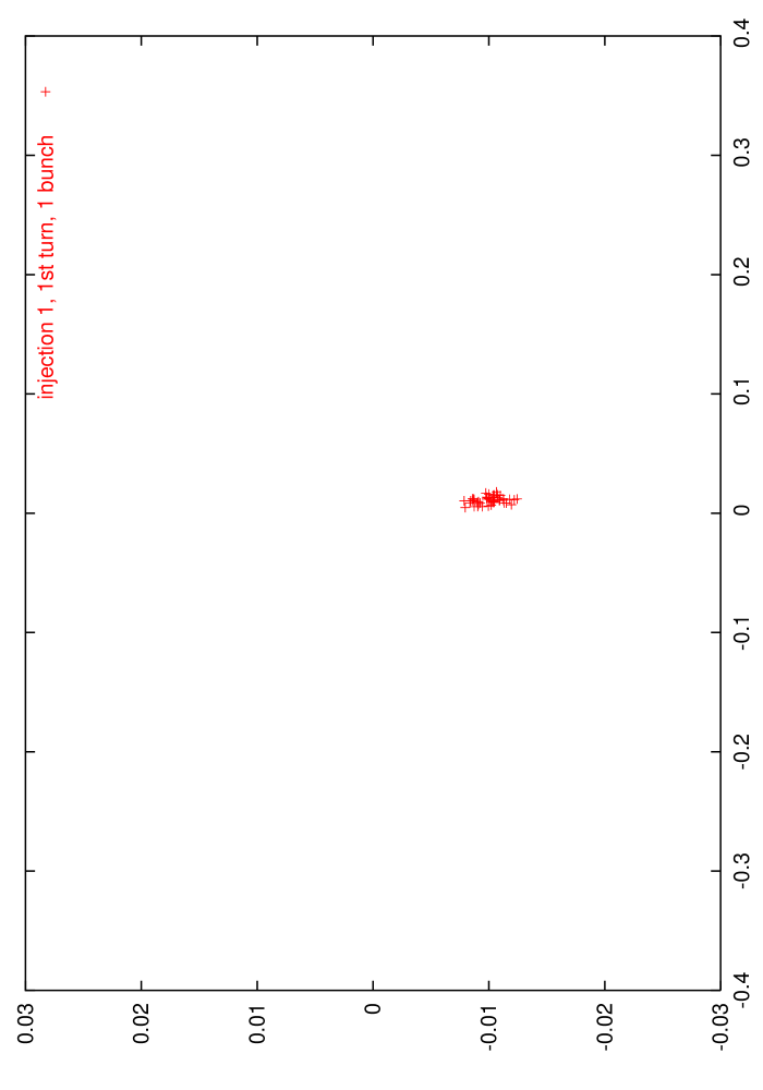
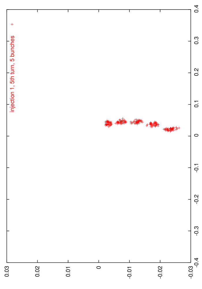
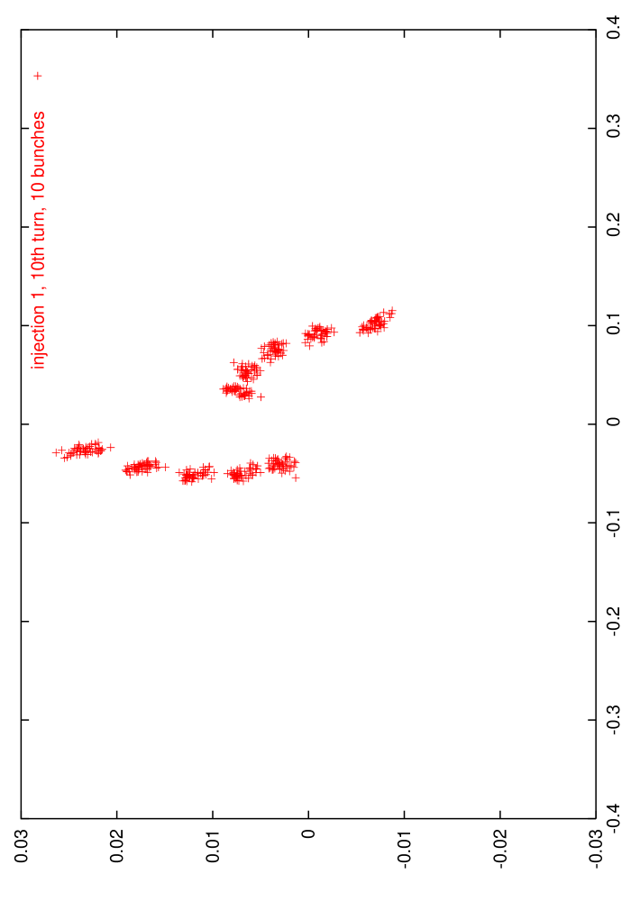
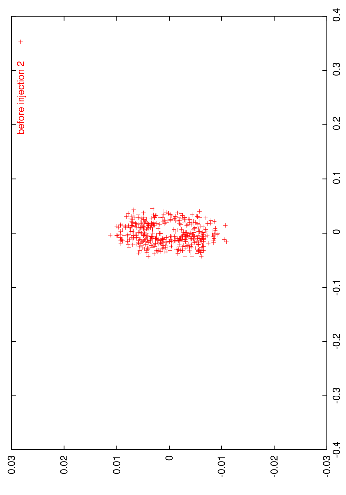
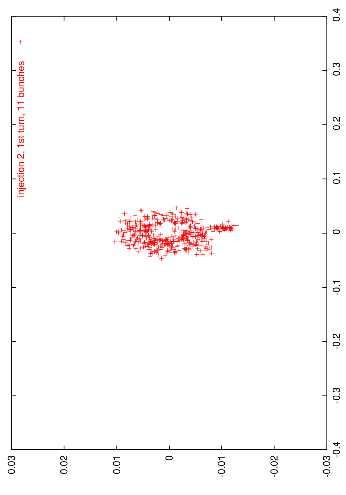
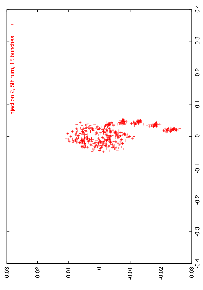
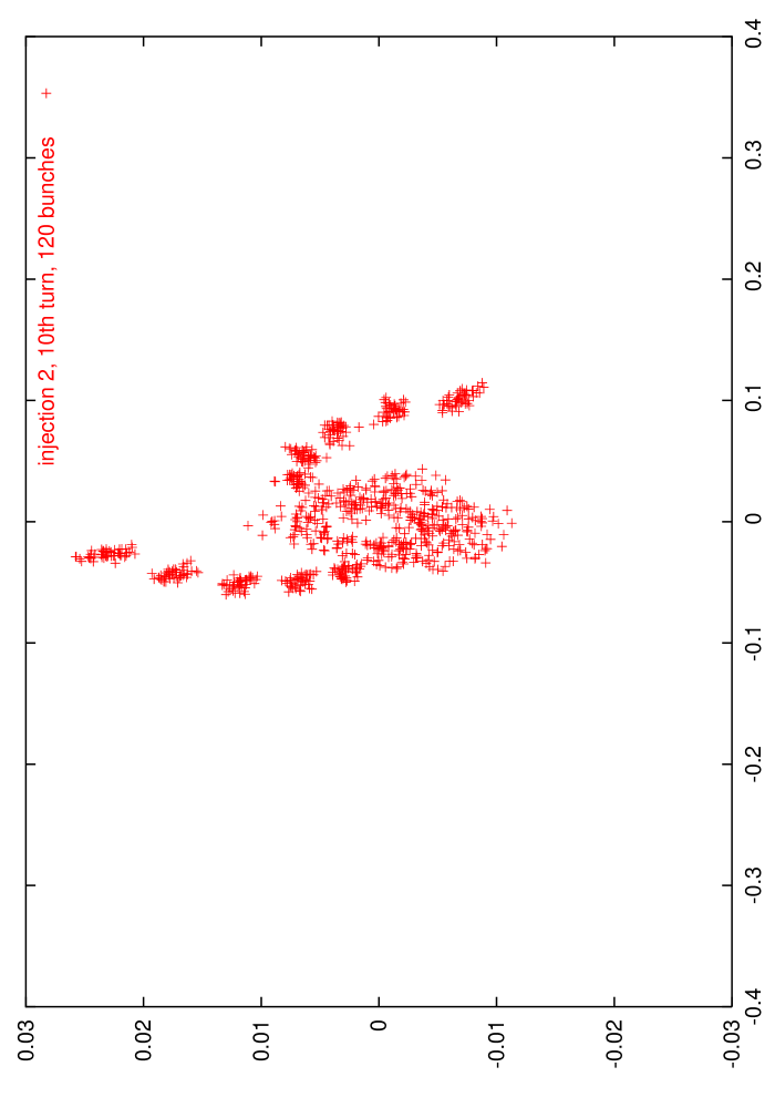
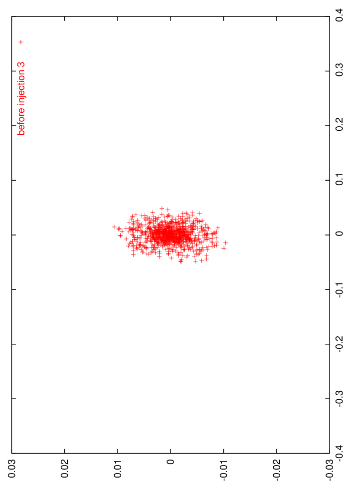
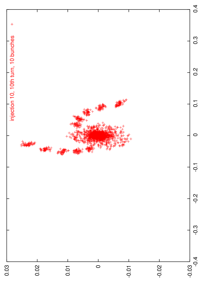
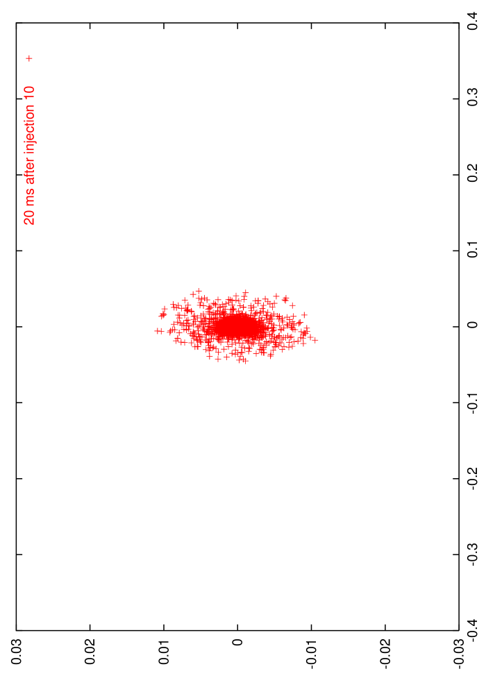
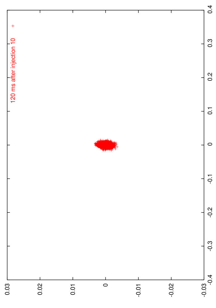
Figure 8: Snapshots of longitudinal phase space during injection and stacking: (a) 1st bunch on 1st turn, (b) 5th bunch on 5th turn, (c) 10th bunch on 10th turn, (d) before 11th bunch on 941st turn, (e) 11th bunch on 942nd turn, (f) 15th bunch on 946th turn, (g) 20th bunch on 951st turn, (h) before 21st bunch on 1882nd turn, (i) 100th bunch on 8479th turn, (j) 100 bunches on 9410th turn, (k) 100 bunches on 18820th turn.

4 Laser System Design

 

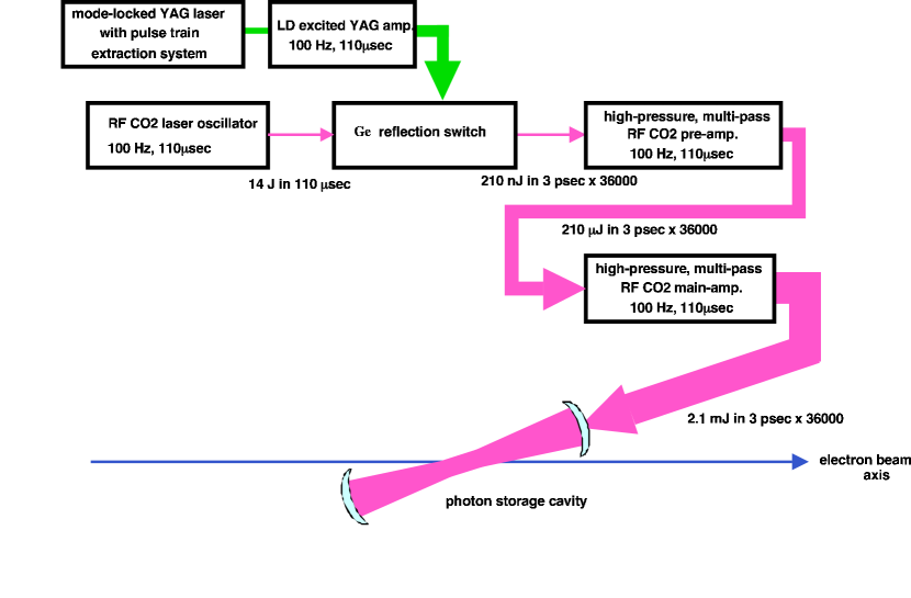
Figure 9: Schematic design of a CO2 laser system.

Figure 9 shows a schematic design of a high-power multi-bunch CO₂ laser system. A long, $\sim 110\mu$s low-energy pulse is generated by a CO₂ laser oscillator operating at 100 Hz. The energy of this long pulse is 14J. To realize such a long pulse, the CO₂ oscillator is pumped by an RF pulse.

This long pulse is sliced into $\sim 3.6\times 10^{4}$ short, 3ps in rms, bunches (seed bunches) by Germanium (Ge )-plates [16], which can switch between reflection and transmission. Each short bunch contains energy of 210nJ.

The reflectivity/transparency of the Ge -plates is controlled by a multi-bunch pico-second YAG laser. The YAG laser consists of a mode-locked laser oscillator and an LD pumped amplifier.

After slicing, $\sim 3.6\times 10^{4}$ CO₂ seed bunches are amplified by a preamplifier and a main amplifier. Gains of the preamplifier and the main amplifier are 1000 and 10, respectively. Both amplifiers are RF-pumped in order to realize long pulse ($\sim 110\mu$s). The preamplifier operates at 100 Hz. For the main amplifier, interleaved 100 Hz operation will be adopted, where the amplifier operates at 100 Hz during 100 ms, and then takes a rest for the next 100 ms. This interleaved mode of operation reduces the average beam power and, therefore, the heat load on the main amplifier.

Finally, we obtain $\sim 3.6\times 10^{4}$ bunches, each of which contains 2.1 mJ and has a bunch duration of $\sim 3$ ps in rms. This short bunch width is necessary in order to match the laser-pulse-length to a depth-of-focus of $\sim 1$ mm for the parabolic-mirrors, which create the final small spot size. To achieve such a short bunch width, the pressure of the CO₂ gas in the pre and main amplifiers must be high (10 atm.).

In the case of a YAG laser system, we need a long, $\sim 92\mu$s, low-energy pulse generated by a 325-MHz modelock 12-W YAG laser oscillator with 10-ps (FWHM) pulse width. To amplify the laser pulse energy from 37 nJ to 6 mJ, four pass amplification is necessary with a long-pulse flash lamp ($\sim 100\mu$s) and with an appropriate cooling system for the flash lamp and the YAG rod.

At this stage, we do not know whether a 100-kW YAG laser system is available or not, but the present laser system of the ATF photo-cathode RF gun can generate about $0.1mJ/pulse$ over 400 pulses from a 357-MHz 6-W laser oscillator by a two-pass amplification. We are planning to increase the pulse train length from $1\mu s$ to $50\mu s$ and implement a 4-pass amplification system. An ultimate technical limit on the maximum power is set by thermal effects on the various elements. If 100-kW YAG operation turns out to be impossible, we have to increase the enhancement factor of the optical cavity from 100 to about 1000. In any case required are a detailed engineering design of the laser system and an experiment on the generation of a huge laser power in the burst operation mode.

If otherwise we want to refer to the existing thin-disk laser head technology (saturable absorber) [17] and associate it with high finesse cavities ( gain 10000 - see appendix A) we will anyway require an enhancement of a factor $\sim 50$ in flux but this scheme has the advantage to work in continuous mode and so with full duty cycle. Therefore the remaining enhancement could be attained working on different parameters:

1. Laser power. The thin-disk laser head technology is very promising and could attain even more power for a single laser in the future.

2. Gain of the cavity. The R&D illustrated in appendix A is foreseen to attain a gain of 10000 in the first phase but a consecutive enhancement of an order of magnitude can be foreseen.

3. The increase of the charge/bunches.

4. Increasing the duty cycle of the positron injection in the damping ring.

5 Compton Collision Chamber Design

 

We assume the basic beam parameters for the ILC main damping ring listed in Table 3. Although there still many parameter options for the main damping ring are being discussed, our scheme of polarised positron generation can be adapted to each option by an appropriate change of the laser system, the Compton-ring design and the 5-GeV injector linac. For simplicity, in this section we describe the design of the Compton collision chamber only for the YAG laser case.

Our group [18] already demonstrated stable operation of the optical cavity with an enhancement factor of 230 using a 42-cm Fabry-Perot optical cavity made of a solid block of super-invar. Also, with this cavity we have conducted a laser-Compton scattering experiment at the ATF damping ring and measured a large rate of $\gamma$ rays consistent with the calculation for a 90-degree crossing angle between the laser and the electron beam [19]. The conceptual setup of this experiment is shown in Figure 10.

In parallel, a Compton scattering experiment dedicated to polarised positron generation has also been done at the ATF, in the extraction line. During the middle stage of this experiment in 2002, we used a short-focus Compton collision chamber consisting of two off-axis parabolic reflective mirrors with a 5-mm diameter hole for the passage of the electron beam [20]. For the next stage, we developed a hybrid optical cavity, in order to both produce a small focal spot size and to increase the enhancement factor. The hybrid cavity consists of two high reflective mirrors (99.9%) and two off-axis parabolic reflective mirrors (also 99.9% reflectivity), shown in Figure 11. The mirrors are mounted on a cylindrical super-invar support equipped with numerous piezoelectric actuators to control the position of the four mirrors and to maintain the resonant condition of the optical cavity. Figure 11 indicates three cylindrical arms with hole on the left and right for the passage of the laser pulse. The middle arm contains another hole for the electron beam.

Figure 12 shows a schematic diagram of the feedback circuit employed to keep the optical cavity on resonance and to control the collision timing, which was used for a first experiment in 2004. This experiment at the ATF damping ring demonstrated a very precise collision control between a 10-ps laser pulse and the electron bunch. The same techniques are also applicable for the Compton collision chamber design of the proposed ILC positron-generation scheme, with the exception of the additional control needed for the distance between two adjacent Compton collision chambers. This inter-chamber distance should equal a large integer multiple of the laser wave length, in order to achieve a high enhancement factor and to maintain the collision timing of the 30 cavities. The position of each Compton collision chamber can be controlled individually, with vacuum bellows between neighbouring chambers. We are aware that an optical cavity with an enhancement factor of 10,000 is under development, but nevertheless we assume only a factor 100 enhancement in order to arrive at a conservative design, given that the serial connection of 30 optical cavities introduces tighter tolerances, which will be estimated after the detailed chamber design is completed.

The conceptual design shown in Figure 13 is our present proposal for the Compton collision chamber, which occupies about 30 m length in the straight section of the Compton ring. We use a FODO lattice to keep the electron beam focused at the Compton ring IP’s.

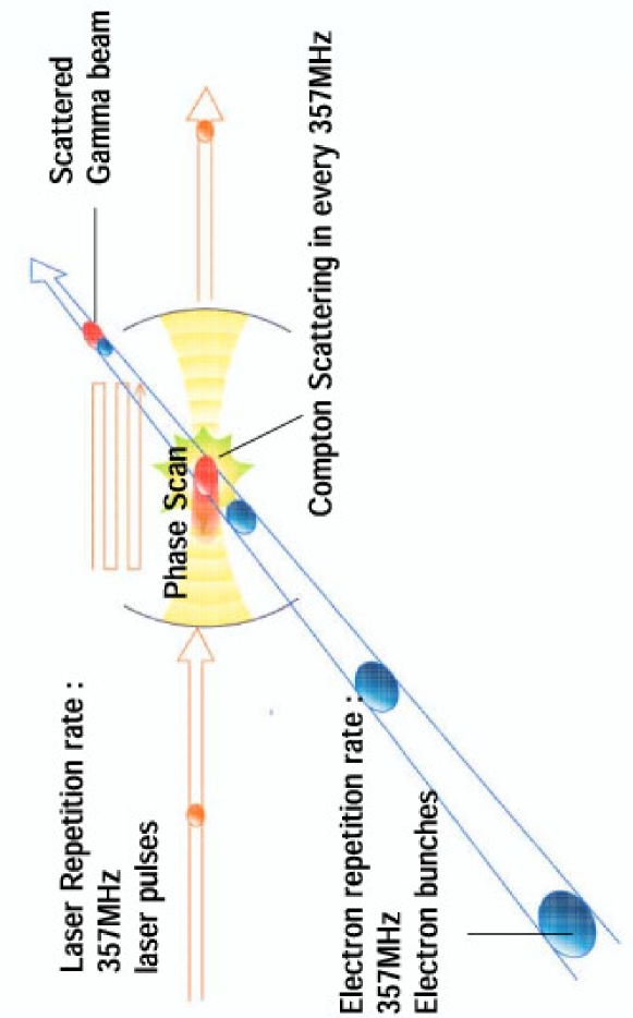
Figure 10: Conceptual view of the Compton scattering experiment in ATF damping ring.

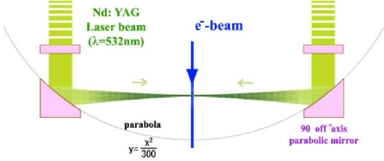
Figure 11: Conceptual view of the ATF Compton chamber for the hybrid optical cavity.

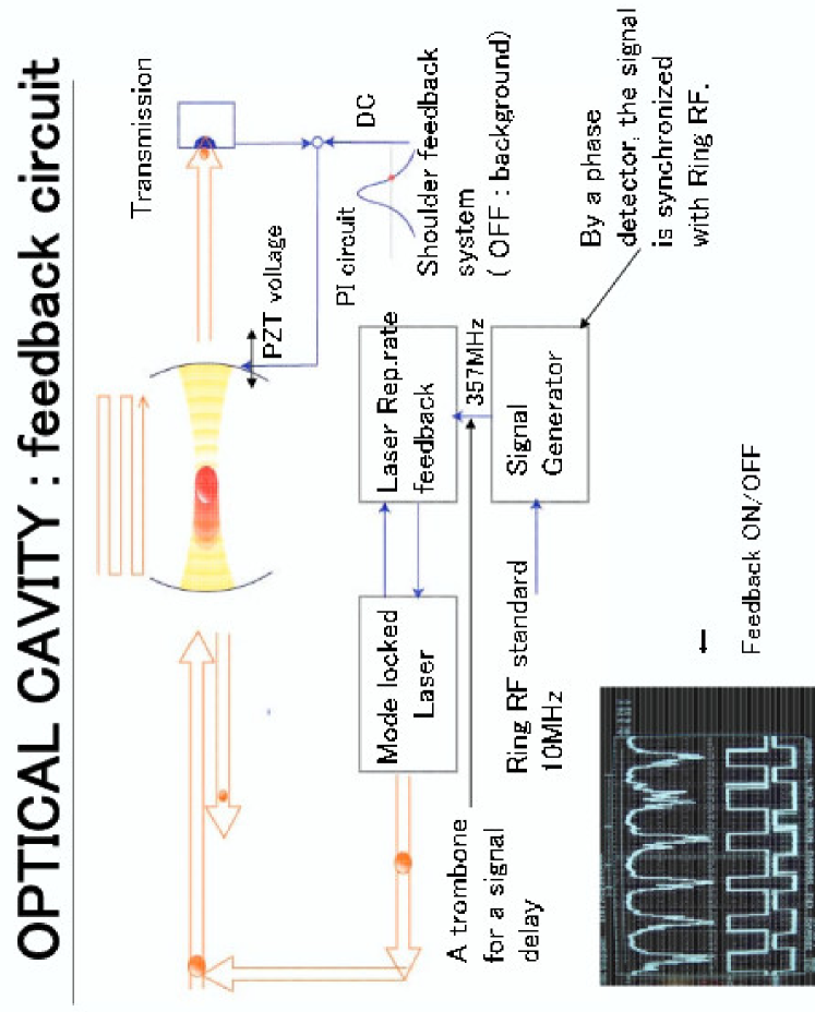
Figure 12: Feedback system for the optical cavity and collision timing control at the ATF.

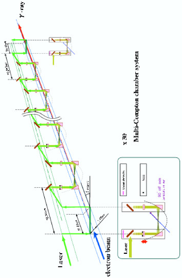
Figure 13: Conceptual view of the proposed Compton collision chamber design.

6 Injector Linac

  The injector linac accelerates the positron beam generated by the Compton system. One pulse contains $\rm 280\times 2\times 50=28000$ or $\rm 280\times 100=28000$ bunches. The bunch spacing is 3.08ns giving $\rm 28000\times 0.000308=86.2\mu s$ pulse length. This pulse is repeated every 10ms, with 100Hz.

If we follow the terminology of TESLA TDR, the injector linac consists from the capture section, PPA(Pre Positron Accelerator), and MPA (Main Positron Accelerator).

For the capture section and PPA, it is hard to use any cold structure due to the heavy radiation loss. On the other hand, for MPA, both technologies, warm and cold, are possible because of the following reasons;

• Average current in a pulse is 10mA. The beam loading does not matter for the warm linac. It does not matter for the cold linac too because it is identical to the main linac. Since I assume that the main linac will be working well, there is no doubt to use the same cavity for the positron acceleration.

• Pulse length is $\rm 86.2\mu s$. It might be critical for the warm linac, but the L-band warm cavity designed for the original TESLA positron capture section, is operated in 0.95ms duration with 14.5 MV/m field. $\rm 86.2\mu s$ pulse operation must be much easier than 0.95ms.

• Repetition is 100 Hz. For the warm linac, the heat load might be critical, but it can be cleared by assuming the same technology in TESLA TDR again. There is no difficulty for the cold linac too because the inter pulse period, 10ms, is even to fill RF power into the cavity whose filling time is $\rm 500\mu s$. All we have to do is pay a small extra cost for the cooling.

In short, MPA based on the warm and cold cavities is possible with the conventional technologies assumed in the ILC project. In the following sections, we will explain PPA based on the warm cavity and MPA with the warm and cold cavities.

6.1 Positron Pre-Accelerator

The Positron Pre-Accelerator, PPA has a role to capture the generated positron. It also defines the acceptance for the positron which should be consistent to the DR acceptance, dynamic aperture.

At this moment, the dynamic aperture is a current issue which will be discussed in the 2nd ILC WS in Snowmass, US, but let us assume $\varepsilon_{x,y}\sim 0.01m.rad$ as a reference. By taking this standard number among the ILC researchers, most of issues related to PPA should be identical to those in other methods, undulator and conventional[21].

In the original TESLA TDR, the PPA is a standing-wave normal-conducting L-band linac[22]. The front end of the PPA consists of acceleration cavities embedded in a focusing solenoid. The first two cavities have a high accelerating gradient ($\rm E_{acc}=14.5MV/m$) and the others have moderate gradients ($\rm E_{acc}=8.5MV/m$). Each cavity is powered by one 10MW klystron.

The only difference of the PPA in the Compton method is the repetition and the pulse duration. The averaged current in a pulse is designed to be identical.

In other methods, the PPA is driven in 5Hz with almost 1ms duration. These numbers are 100Hz with 100ms interval with almost $\rm 100\mu s$ duration in this method. The heat load to the cavity is estimated to be exactly same as that in the other method since the ratio of the heat load to that of the other methods, $C_{hl}$ is accounted as

$$C_{hl}=\frac{100}{5}\times\frac{100}{1000}\times\frac{1}{2}=1.0,$$ (11)

where the first fraction comes from the repetition rate, the second term means the ratio of the pulse duration, and the last term means the duty cycle, i.e. the cavity is driven in half of every 100ms.

¿From this simple estimation, we do not have to pay any extra cost to drive the PPA with this high repetition and short duration mode. We do not need any modification on the PPA.

The gradients in the first and second cavities of the PPA are limited by RF power and heat load restrictions. Three dimensional thermal stress analysis indicates that stable and reliable cavity operation with a heat load of about 30 kW/m is possible, corresponding to an accelerating gradient $\rm E_{acc}=14.5MV/m$ with the long RF pulse ($\rm 950\mu s$ flat-top) and repetition rate of 5Hz[23]. The heat load of the cavity in the same gradient with the high repetition and short duration is identical, this statement is therefore also true for our case.

The rest of the PPA consists of five cavities with moderate gradient (8.5MV/m) as same as that in TESLA TDR[22]. Each cavity has two accelerating sections. The transverse focusing is accomplished using quadrupole triplets, placed between the sections. Each cavity is powered by one 10MW klystron.

At the exit of the PPA section, 287 MeV bunched positron beam is obtained.

6.2 MPA based on the warm technology

In MPA, the same technology as the latter part of the PPA section can be used to accelerate the beam up to 5 GeV.

One accelerating module consists from two accelerating sections and quadrupole triplets[23]. Total length of the module is 4.3m. The energy gain per one module is 34.6 MeV. To accelerate the positron beam up to 5 GeV, 144 modules are required including 5% of the margin. The total length of the linac becomes 690m including 0.5m for the quadrupole triplets inserted between the modules. One module is driven by one 10MW klystron, so that totally 144 klystron is needed. The parameters of MPA based on the L-band warm structure, are summarised in Table 4.

Table 4: Parameters of the injector linac based on the L-band warm structure.

Item	number	unit
Field gradient	8.5	MV/m
Energy gain per module	34.6	MeV
Number of module	144	unit
Number of klystron	144	unit
Total length	620	m

6.3 MPA based on the cold technology

If we employ the cold technology for MPA, we can use the system almost identical to that of the main linac. The bunch spacing is 3.08 ns which is 100 times smaller than that in the main linac, but the bunch intensity is only 0.03nC giving the exactly same average current, 10mA. Because of this fact, we can use the same cavity and coupler including the coupling coefficient.

If the cavity is operated in 100 Hz repetition with $\rm 100\mu s$ duration, the heat load generated when the beam is on, can be identical to that in the main linac because of the same average current and effective pulse duration, $100\mu s\times 10=1ms$. The heat load coming from the RF filling and decay time, however, contribute and dominates the total heat load.

If the heat load from the RF filling and decay period corresponds to that of $\rm 500\mu s$ of the beam period, the multiplication factor of the total heat load of the Compton operation mode against to that of 1ms operation, $C_{RF}$ is

$$C_{RF}=\frac{500\times 10+100\times 10}{1000+500}=4.0$$ (12)

We need therefore 4 times larger cooling power to operate MPA in the Compton mode. This excess shares, however, only $\rm 15/(500+500+5+5)=1.4$% and $\rm 15/(1000+1000+5+5)=0.7$% of the total heat load in the whole ILC 500 and 1000 respectively.

By considering the large emittance compared to the main linac, we have to employ a same arrangement of the cryomodule of that in TESLA TDR. To achieve enough focusing to accelerate the positron beam which has a large emittance, two types of the cryomodule assemblies are designed[22].

The cryomodule for MPA is implemented from the two types of the standard ILC cryomodules. The transverse focusing is carried out by quadruples doublets. Type 1 module consists from four accelerator cavities and four quadrupole doublets. Type 2 module consists from 8 accelerator cavities and 1 quadrupole doublets. The length of the cryomodules are 11.4m and 12.4 m for type 1 and type 2 respectively.

In the TESLA TDR, the field gradient in the cavity is assumed to be 25 MeV/m[22]. If we employ 35 MV/m which is likely to be a new standard of the field gradient in ILC, the energy gain per the module can be 140 and 280 MeV/module for type 1 and 2 respectively. Assuming this higher acceleration field than that in TESLA MPA module, we can reduce the number of the modules to be 6 of type 1 and 15 of type 2. Number of modules in the original TESLA TDR was 8 of type 1 and 20 of type 2.

The total energy gain of MPA is estimated to be 5040 MeV. Including the energy gained by PPA, the final energy of the positron beam becomes 5290 MeV which is even enough by assuming 5% margin. Total length of MPA becomes 270m. This number includes 0.5m for the inter-module bellows section and 5m for the cooling channel. One 10MW klystron can drive 10 cavities with 35 MV/m gradient[25]. Total number of cavities in MPA is 139 which requires 14 klystrons. Considering a margin, let us assume 3 klystrons for 6 type1 modules and 12 klystrons for 15 type 2 modules. The total number of klystrons is 15. Parameters of MPA based on the cold cavity are summarised in Table5.

Table 5: Parameters of MPA based on the cold technology.

Item	Number	unit
Number of type 1 module	6	unit
Module length	11.4	m
Energy gain/module	140	MeV
Number of quadrupole doublets	4	unit
Number of cavities	4	unit
Number of type 2 module	15	unit
Module length	12.4	m
Energy gain/module	280	MeV
Number of quadrupole doublets	1	unit
Number of cavities	7	unit
Final energy	5.29	GeV
Total length	270	m
Total number of cryomodules	21	unit
Total number of klystrons	14	unit

7 Total System

 

Figures 14 and Figure 15 illustrate the total system for two versions of our proposal.

The first represents the case of YAG laser Compton scattering. It assumes that one train (280 bunches) of the electron beam is stably circulating in the Compton ring except for the period of the Compton scattering (100Hz, about $100\,\mu$s pulse width, duty factor $50\%$ ). Electron losses are not problem, but bunch lengthening is a concern since the $\gamma$-ray yield depends on the bunch length due to crossing angle. From our beam tracking simulation for the Compton ring, we infer that the beam loss is negligible and that the electron bunch recovers in about 9.9 ms after a 100-turn burst collision. A more detailed design study and optimisation of the Compton ring will necessary prior to construction. This $\gamma$-ray generation scheme requires a 100-Hz 5-GeV injector linac after the conversion target and 10 times successive beam stacking into each bunch of the main damping ring, which is repeated for 10 linac pulses. If we assume appropriate beam parameters, the beam tracking simulation for the damping ring shows that 10 times successive beam stacking is possible. The conceptual design of the Compton collision chamber and the laser system are described in Sections 5 and 6.

A preliminary Compton collision experiment has been performed using pulsed YAG laser (10ps FWHM) and a simple Fabry-Perot optical cavity with a 90-degrees crossing angle. The state of art was already demonstrated with about a factor 100 enhancement of the optical cavity, except for technologies and issues related to a small crossing angle geometry and the more strongly focused laser beam size. The experimental test of a double Compton-chamber system is necessary and under planning at the ATF damping ring.

An alternative system uses a CO2 laser. The principle of this scheme is analogous the case of the YAG laser. One difference is that the beam energy in the CO2-laser Compton ring is 4.1 GeV instead of 1.3 GeV for the YAG laser. The CO2 laser uses a 50-turns burst collision, instead of a 100-turn collision, The 50-turns collision generates sufficient $\gamma$-rays in the Compton ring, which has a larger circumference and stores a beam of two trains (2x280 bunches).

The average positron population of the injected bunches is about $2\times 10^{8}$ for either laser, and this intensity changes dynamically by a factor of about 4 during the Compton collisions. Since the beam loading is very small, we do not expect any problem in the 5-GeV injector linac and can control the stacking beam intensity in the main damping ring. The most important outstanding technical issues are to develop the laser system and the Compton collision chamber.

The polarised-positron generation scheme which we propose is very flexible, and of moderate size. It provides a fully independent system which means that we can perform the ILC beam commissioning at full beam power without the need of a 150-GeV electron beam. The design of the Compton ring, the Compton collision chamber, and the laser system will be optimised with respect to tolerances.

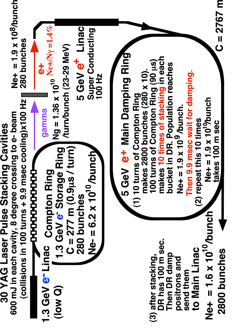
Figure 14: Schematic diagram of the total system in the case of YAG laser.

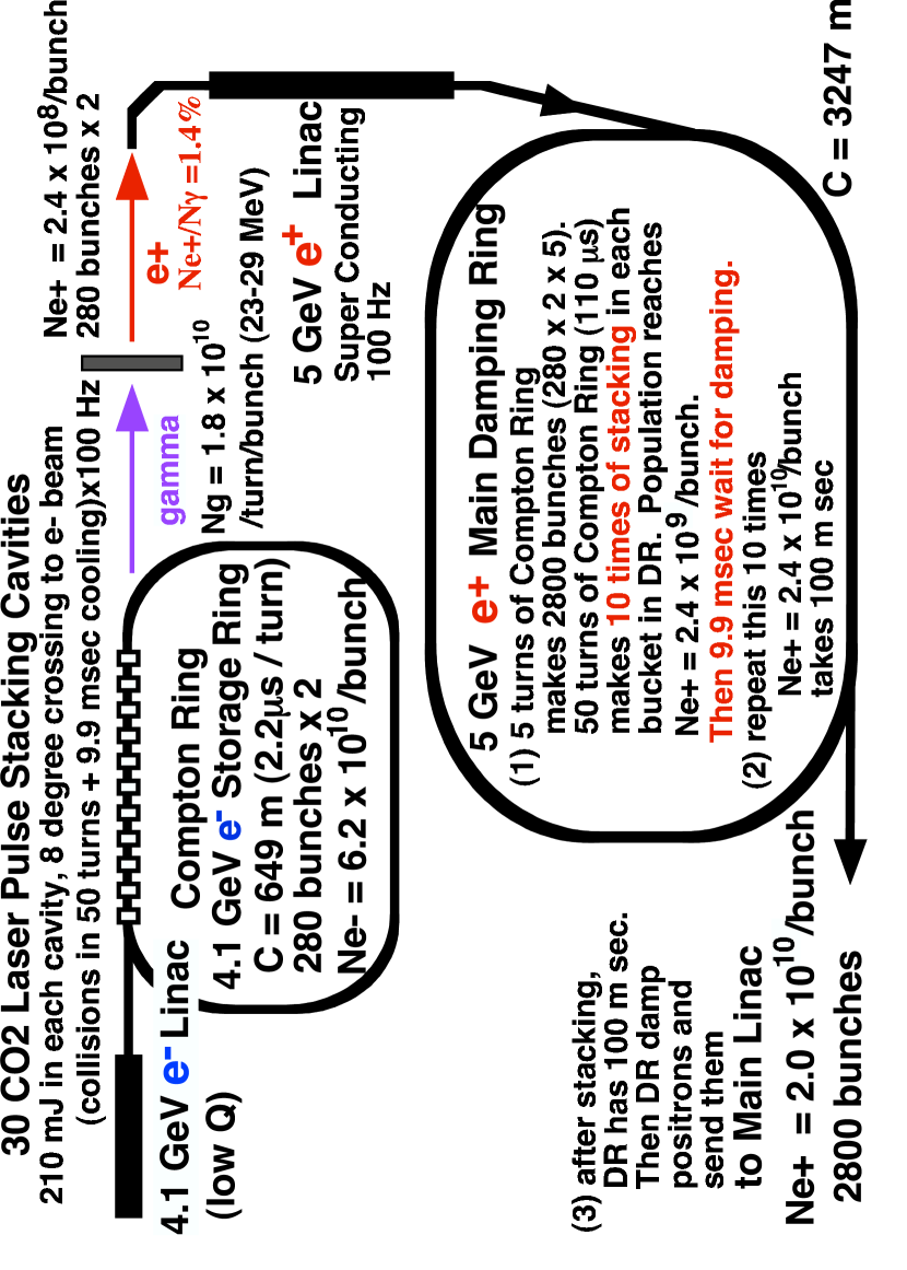
Figure 15: Schematic diagram of the total system in the case of CO2 laser.

Appendix A Cavity R&D in Orsay

 

A.1 Introduction

The envisaged high finesse of around 30000 has already been reached for cavities filled with a continuous Nd:YAG laser beam in polarimeters used at CEBAF [26, 27, 28] and DESY [29]. Also some cavities are already working in the pulsed regime. At SLAC a cavity with 30 ps pulses reached a finesse of 12000 [30]. At KEK a pulsed cavity is built for a laser wire application [18].

A.2 Description of present project

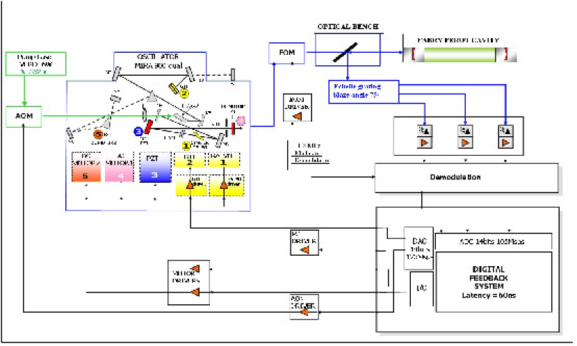
Figure 16: Schematic view of the feedback system. See text for a description of each component. In the MIRA oscillator, mirrors M6, M7 and M9 (M10 being removed) and the two prisms P1 and P2 are used in the 100fs regime. In the 1ps, the prism P1 is moved away from the optical path and M10 is inserted. The Lyot filter [39] and the output coupler M1/OC are also changed.

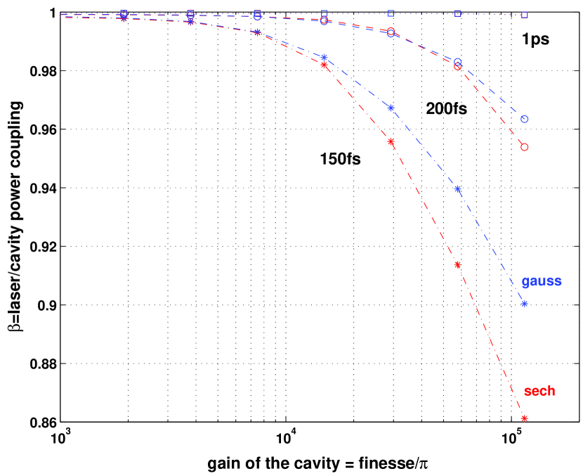
Figure 17: Laser-beam/cavity-beam coupling as a function of the gain of a 2m long Fabry-Perot cavity. Only the chromatic dispersion effects in the cavity mirror coatings are taken into account in the coupling calculation. To pulse shapes are considered: a Gaussian and a soliton (denoted by sech on the figure).

Our R&D is an investigation on whether a high finesse Fabry-Perot resonator [31] can be used to ‘amplify’, with an energy gain ranging from $10^{4}$ to $10^{5}$, a passive mode-locked laser beam [32]. This would allow a drastic gain in the Compton cross section once that the cavity is located around the electron beam. Two pulse laser time widths will be tried: full width at half maximum (FWHM) of 100fs and 1ps.

In a first step, a confocal (mechanically stable) two mirrors cavity will be considered. High quality mirrors will be mounted in order to reach cavity finesses of 30000 and 300000 (i.e. power gain of 10000 and 100000). In a second step, a more complex resonator will be considered to reduce the laser beam waist inside the cavity : a concentric cavity (mechanically unstable) made of two mirrors or a four-mirror cavity. This second step is still under study at the present time. Both steps require a special mechanical design of highly stable cavity mirror mounts and a great care on the reduction of the environment noise.

In principle, the smaller the pulse time FWHM the larger the laser frequency spectrum. One then expects that chromatic dispersion induced by the pulse propagation in the multilayer mirror coatings [33, 34, 35] and the finite frequency bandwidth of these coatings [36] will reduce the coherent coupling of the incident laser pulses to the pulse circulating inside the cavity. We performed these calculations for soliton and Gaussian like pulses. The cavity mirror reflection coefficients were calculated numerically using standard multilayers formula [37] including the values of the optical indices as given by our mirror coating manufacturer [38]. Fig. 17 shows the effective cavity gain $\beta$ as a function of the gain of a 2m long Fabry-Perot cavity (i.e. the number of double layers constituting the cavity mirror coating). From this figure one sees that this effect is negligible for 1ps FWHM whereas the coupling of the incident power is reduced by $\approx 14\%$ for 150fs FWHM. Pulses with time FWHM as small as 150fs can therefore be envisaged to be efficiently ‘amplified’ in a very high finesse Fabry-Perot cavity. Note that passive mode locked laser pulses have a time shape closed to that of a soliton.

The experimental scheme of the first step of our R&D is shown in Fig. 16. A commercial passively mode locked laser, Coherent’s MIRA Ti:sa oscillator with 76MHz pulse repetition rate, pumped by a green laser beam, Coherent’s 6W VERDI, is sent into a Fabry-Perot cavity. The laser is locked to the cavity by means of the Pound-Dever-Hall technique [40] adapted to the pulsed laser beam regime [41, 42, 43, 44, 45]. Following our estimation both the laser pulse repetition rate $f_{rep}$ and the phase shift between the carrier and the envelope of the electric field $\varphi_{ce}$ [46] must be locked to the Fabry-Perot cavity in the two pulse length regimes (1ps and 100fs). To perform this locking, at least two error signals are necessary. To build the error signals, the laser beam is phase modulated by an Electro-Optic-Modulator (EOM) and the signal reflected by the cavity is sent to a diffraction echelle grating. The intensity is then read at different positions, that is at different values of the wavelength. After demodulation, these signals are sampled and analysed by a digital feedback system (Lyretec XXX card). Correction signals are built and sent to various actuators according to their frequency bandwidths and functionalities:

• an Acousto-Optic-Modulator (AOM), used as an amplitude modulator for the pump laser beam to control the fast variations of both $f_{rep}$ and $\varphi_{ce}$ [48];

• a fast piezoelectric transducer glued on one of the oscillator mirror to control the fast variations of $f_{rep}$;

• a galvometer on which is located the mode locking starter (= two mirrors) to follow the slow drifts of $f_{rep}$;

• a translation stage on which is located the oscillator output coupler to adjust roughly the oscillator length to the Fabry-Perot cavity length;

• a piezoelectric transducer acting on the width between the platelets of the Gire-Tournois (GTI) interferometer [47]. With this actuator, one is able to follow the slow drifts of $\varphi_{ce}$ in the 1ps version of the MIRA ($f_{rep}$ being also affected).

• a translation stage on which is located one of the prism in order to control the slow variations of $\varphi_{ce}$ in the 100fs version of the MIRA ($f_{rep}$ being also affected).

The feedback strategy is not, and cannot [48], be defined a priori, i.e. one must calibrate the pump and oscillator lasers to define which actuators must be used in conjunction with a given error signal. This calibration depends on our lasers and on the environment noises. To calibrate the actuator responses, we shall follow the methods of ref. [48, 49]. To characterise the phase and amplitude laser noises [50], we shall use the setups of refs. [51, 52]. With our ’long’ pulses, an autocorrelator [53] will be used to observe the variations of $\varphi_{ce}$ during the calibration experiments. As for $f_{rep}$, a spectrum analyser and a large band oscilloscope will be used. Finally, the beam pointing stability of the pump laser beam will be determined as described in [49].

As previously mentioned, the mechanical stability will play a fundamental role in the second phase, where we envisage to pass from a confocal configuration to a concentric one. This will allow us to obtain a much smaller waist size in the Fabry Perot resonator,thus increasing the photon density in the interaction point.

The main problem is that the concentric configuration is highly mechanically unstable.

As an example we can say that in our 2m long cavity a waist of around 130 microns can be obtained with a 1 cm separation between the two centres of curvature of the two mirrors. This will imply a maximum range of stability that corresponds to less than 10 microradian in tilt (for this tilt the optical axis is out of the cavity). Reducing the waist size will require more stringent constraints.

Therefore much attention will be paid to the environmental noise suppression and for the optical table passive stabilisation. The two mirrors of the cavity will be mounted on separate holders allowing an independent distance regulation.

Furthermore, to approach this problem we have studied a new mirror holder system (see fig 2) that will be tested on the confocal cavity as a proof of principle. The principle of this holder is based on a monoblock cardan joint system that allows both rotations around the geometrical centre of the mirror. Thanks to its specificity this system is based on simple flexions, thus avoiding backlask and friction. The external tilt adjustment is assured by a wedge system.

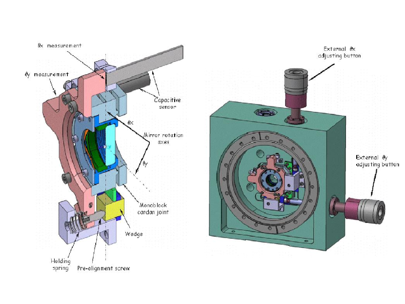
Figure 18: Mirror holder prototype

This avoids the stacking of different elements (therefore adding vibration sources), minimises the distance between the regulation point and the support, and the mechanical coupling with the environment. A very good sensitivity for the displacement is ensured by the high demultiplication factor that gives a precision of $\approx$ 0.5 microradian. A capacitive sensor is installed to measure the mechanical stability and the tilt and to eventually provide the signal for an active feedback. This is installed on the support and reads the distance between the support itself and the mirror holder. The resolution is 20 nm at 1 kHz of acquisition rate.

References

- [1] G. Moortgat-Pick et al., arXiv:hep-ph/0507011.
- [2] A. Mihailichenko, Use of Undulators at High Energy to Produce Polarized Positrons and Electrons, SLAC-R-0502 (1997) 229.
- [3] T. Omori et al., Nucl. Inst. Meth. A500 (2003) 232.
- [4] I.I. Goldman. Intensity effects in Compton scattering, Sov.Physics JETF, 46:1412–1417, 1964.
- [5] A. Kh. Khokonov and M. Kh. Khokonov, Classification of the interactions of relativistic electrons with laser radiation., Technical Physics Letters, 31(2):154–156, 2005.
- [6] J. J. Thomson. Conduction of Electricity through Gases. Cambridge Univ. Press, 1906.
-
[7]
Eugene Bulyak and Vyacheslav Skomorokhov,
Parameters of x–ray radiation emitted by Compton sources,
In Proc. EPAC–2004 (Luzern, Switzerland), 2004,
http://accelconf.web.cern.ch/accelconf/e04/papers/weplt138.pdf. - [8] Eugene Bulyak. Laser cooling of electron bunches in Compton storage rings, In Proc. EPAC–2004 (Luzern, Switzerland), 2004, http://accelconf.web.cern.ch/accelconf/ e04/ papers/thpkf063.pdf.
- [9] Peter Gladkikh, Lattice and beam parameters of compact intense x-rays source based on Compton scattering, Phys. Rev. ST Accel. Beams, 8:050702, 2005.
- [10] J. Feikes, K. Holldack, P. Kuske, G. Wüstefeld, and H.-W. Hübers, The BESSY low alpha optics and the generation of coherent synchrotron radiation, ICFA Beam Dynamics Newsletter, 35:82–95, 2004.
- [11] Eugene Bulyak, Peter Gladkikh, and Vladislav Skomorokhov. Synchrotron dynamics in Compton x–ray ring with nonlinear compaction, In arXiv, page 5 p. physics/0505204v1, 2005.
- [12] J. Yang, M Washio, A. Endo, and T. Hori. Evaluation of x–rays produced by Thomson scattering under interactions between electron beam and laser light, Nucl. Instrum. Methods, A 428:556–569, 1999.
- [13] K. Flöttmann, private communication (2005).
- [14] S. Krishnagopal, R. Siemann, Simulation of Round Beams, PAC 1989, Chicago (1989)
- [15] A. Wolski, Damping-Ring Megatables, http://www.desy.de/ãwolski/ILCDR/Lattices.htm
- [16] I. V. Pogorelsky et al., IEEE J. Quantum Electron., 31 (1995) 556.
- [17] E. Innerhofer et al., Opt. Lett. 28 (5), 367 (2003).
- [18] M.Nomura et al., Enhancement of Laser Power from a Mode Lock Laser with an Optical Cavity, p.2637-2639, Proceedings of EPAC 2004, Lucerne, Switzerland.
- [19] K. Takezawa, master thesis submitted to Kyoto University (2004).
- [20] I.Sakai et al., Production of high brightness g rays through backscattering of laser photons on high-energy electrons, Physical Review Special Topics-Accelerators and Beams, 6, 091001(2003).
- [21] Edited by J. Sheppard et al., ILC POSITRON SOURCES WRITE-UPS
- [22] R. Brinkmann et al., TESLA Technical Design Report Part II: The accelerator, DESY-01-011B.
- [23] K. Flöttmann, V. Paramonov ed., Conceptual design of a Positron Pre- Accelerator for the TESLA Linear Collider, DESY TESLA-99-14, 1999.
- [24] V. Paramonov, I. Gonin, 3D Thermal Stress Analysis for the CDS Structure, Proc. 7th EPAC, Vienna 2000, p. 1990.
- [25] K. Saito, private communication.
- [26] N. Falletto, Etude, conception et réalisation d’une cavité Fabry-Perot pour le polarimètre Compton de TJNAF, Ph.D. Thesis, Université Joseph Fourier-Grenoble 1, 1999. DAPNIA/SPhN-99-03T.
- [27] N. Falletto et al., Nucl. Instrum. Meth. A459 (2001) 412.
- [28] M. Baylac et al., Phys. Lett. B539 (2002) 8.
- [29] F. Zomer, Habilitation, Université Paris 11-Orsay (2003) LAL/0312.
- [30] R.J. Loewen, A compact light source: design amd technical feasability study of a laser-electron storage ring X-ray source, SLAC-Report-632 (2003).
- [31] H. Kogelnik and T. Li, Proc. of the IEEE 54 (1966) 1312.
- [32] F. Krautz et al., IEEE J. Quant. Elec. 28 (1992) 2097.
- [33] R. Jason Jones and J. Ye, Opt. Lett. 27 (2002) 1848.
- [34] R.J. Jones and J. Ye, Opt. Lett. 29 (2004) 2812.
- [35] J.C. Petersen and A.N. Luiten, Opt. Exp. 11 (2003) 2975.
- [36] C.J. Hood et al., Phys. Rev. A64 (2001) 033804.
- [37] P. Yeh, Optical Waves in Layered Media (Wiley, New York, 1988)
-
[38]
Laboratoire des Mat’eriaux Avanc’es,
http://lma.in2p3.fr/ - [39] See, for example, B. Cagnac and J.-P. Faroux Lasers, p312 (CNRS Editions, Paris 2002).
- [40] R.W.P. Drever et al., Appl. Phys. B 31 (1987) 97. See also E.D. Black, Am. J. Phys 69 (2001) 82.
- [41] R.J. Jones et al., Opt. Comm. 175 (2000)409.
- [42] E. O. Potma et al., Opt. Lett. 28 (2003) 1835.
- [43] Y. Vidne et al., Opt. Lett. 28 (2003) 2396.
- [44] R.J. Jones et al., Phys. Rev. A69 (2004) 051803.
- [45] S.T. Cundiff and J. Ye Femtosecond optical frequency comb technology, (Springer 2005).
- [46] Th. Udem et al., Opt. Lett. 24 (1999) 881.
- [47] J.Desbois et al., C. R. Acad. Sci (Paris) ser. B, vol. 270 (1970) 1604.
- [48] K.W. Holman et al., IEEE J. Sel. Top. Quant. Elec. 9 (2003) 1018.
- [49] S. Witte et al., Appl. Phys. B 78 (2004) 5.
- [50] H.A. Haus, IEEE J. Quant. Elec. 29 (1993) 983.
- [51] R.P. Scott et al., IEEE J. Sel. Top. Quant. Elec. 7 (2001)641.
- [52] E. N. Ivanov et al., IEEE Trans. Ultraso., Ferro., Freq. Contr. 50 (2003)355.
- [53] L. Xu, C. Spielmann, A. Poppe, T. Brabec, F. Krausz and T.W. Hänsch, Opt. Lett. 21 (1996) 2008.