Equilibrium Conditions for the Floating of Multiple Interfacial Objects

Abstract

We study the effect of interactions between objects floating at fluid interfaces, for the case in which the objects are primarily supported by surface tension. We give conditions on the density and size of these objects for equilibrium to be possible and show that two objects that float when well-separated may sink as the separation between the objects is decreased. Finally, we examine the equilbrium of a raft of strips floating at an interface, and find that rafts of sufficiently low density may have infinite spatial extent, but that above a critical raft density, all rafts sink if they are sufficiently large. We compare our numerical and asymptotic results with some simple table-top experiments, and find good quantitative agreement.

1 Introduction

A common table-top demonstration of the effects of surface tension is to float a metal needle horizontally on water: even though the density of the needle is much greater than that of water, the needle is able to remain afloat because of the relatively large vertical component of surface tension. This effect is a matter of life or death for water-walking insects Bush & Hu (2006), and is also important in practical settings such as the self-assembly of small metallic components into macroscopic structures via capillary flotation forces Whitesides & Grzybowski (2002). In this engineering setting an object should not only float when isolated at the interface, but must also remain afloat after it has come into contact with other interfacial objects, and portions of the meniscus that supported it have been eliminated. Although the interactions that cause interfacial objects to come into contact and form clusters have been studied extensively (see, for example, Mansfield, Sepangi & Eastwood, 1997; Kralchevsky & Nagyama, 2000; Vella & Mahadevan, 2005), the implications of such interactions on the objects’ ability to remain afloat have not been considered previously.

Here we consider the effects of these interactions via a series of model calculations that shed light on the physical and mathematical concepts that are at work in such situations. For simplicity, the calculations presented here are purely two-dimensional, though the same physical ideas apply to three-dimensional problems.

2 Two horizontal cylinders

Perhaps the most natural way to characterise the effects of interaction is to ask how the maximum vertical load that can be supported by two floating cylinders varies as the distance between them is altered. We thus consider two cylinders of infinite length lying horizontally at the interface between two fluids of densities $\rho_{A}<\rho_{B}$, as shown in figure 1. We assume that these cylinders are non-wetting so that the contact angle $\theta$, a property of the three phases that meet at the contact line, satisfies $\theta>\pi/2$.

We non-dimensionalise forces per unit length by the surface tension coefficient, $\gamma_{AB}$, and lengths by the capillary length, $\ell_{c}\equiv(\gamma_{AB}/(\rho_{B}-\rho_{A})g)^{1/2}$, and use non-dimensional variables henceforth. We wish to determine the maximum weight per unit length, $W$, that can be supported by each of two identical cylinders with radius $R$ and centre–centre separation $2\Delta$.

To remain afloat each individual cylinder must satisfy a condition of vertical force balance: their weight (or other load) must be balanced by the vertical contributions of surface tension and the hydrostatic pressure acting on the wetted surface of the cylinder. We assume that an external horizontal force is applied to maintain the separation of the cylinders and so do not consider the balance of horizontal forces explicitly.

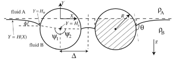
Figure 1: Cross–section of two parallel, horizontal cylinders lying at an interface with a non-dimensional centre–centre separation of $2\Delta$.

Using the notation of figure 1, the vertical force balance condition may be written $W=U_{1}+U_{2}$ where

$$U_{i}\equiv-\sin(\theta+\psi_{i})-H_{0}R\sin\psi_{i}+\tfrac{1}{2}R^{2}(\psi_{i}+\sin\psi_{i}\cos\psi_{i})\hskip 14.22636pt(i=1,2),$$ (1)

are the contributions to the vertical upthrust provided by the deformation on each half of the cylinder separately, and $H_{0}$ is the height of the cylinders’ centres above the undeformed free surface. Physically, the first term on the right hand side of (1) is the vertical component of surface tension, and the second and third terms quantify the resultant of hydrostatic pressure acting on the wetted perimeter of the cylinder. The latter is given by the weight of water that would fill the dashed area in figure 1 (see Keller, 1998).

The angles $\psi_{1}$ and $\psi_{2}$ are determined by the interfacial shape, which is governed by the balance between hydrostatic pressure and the pressure jump across the interface associated with interfacial tension. This balance is expressed mathematically by the Laplace–Young equation. In two dimensions this is

$$H_{XX}=H(1+H_{X}^{2})^{3/2},$$ (2)

where $H(X)$ is the deflection of the interface (again measured positive upwards) from the horizontal, and subscripts denote differentiation. Since the exterior meniscus extends to infinity, the first integral of (2) is particularly simple in this instance and allows the height of the contact line, $H_{*}$, to be related to the interfacial inclination, $\phi$, via

$$\cos\phi=1-\tfrac{1}{2}H_{*}^{2}.$$ (3)

This, together with the geometrical condition $\phi=\theta+\psi_{1}-\pi$, allows $\psi_{1}$ to be eliminated from (1) in favour of $H_{0}(=H_{*}+R\cos\psi_{1})$ and $\theta$.

For the interior meniscus, we simultaneously obtain $\psi_{2}$ and the shape $H(X)$, by using the MATLAB routine bvp4c to solve the nonlinear eigenproblem

$$H_{XX} =H(1+H_{X}^{2})^{3/2},$$ (4)

$$H_{X}(R\sin\psi_{2}) =\tan(\theta+\psi_{2}),$$

$$H(R\sin\psi_{2}) =H_{0}-R\cos\psi_{2},$$

$$H_{X}(\Delta) =0,$$

on $[R\sin\psi_{2},\Delta]$.

With the angles $\psi_{1}$ and $\psi_{2}$ calculated, $W(H_{0})$ can be determined from (1), and the maximum load that can be supported, $W_{\mathrm{max}}$, can be found numerically by varying $H_{0}$. Of particular interest is the dependence of $W_{\mathrm{max}}$ on the cylinder separation, which is shown for several values of the Bond number $B\equiv R^{2}$ in figure 2. This plot includes the limiting case $B=0$, corresponding to the application of two point forces to the interface.

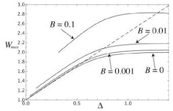
Figure 2: Numerical results for the maximum load that can be supported by a single cylinder in the presence of another a distance $2\Delta$ away when $\theta=2\pi/3$ for several values of the Bond number, $B\equiv R^{2}$. The dashed line shows the linear approximation (5) for the limiting case $B=0$ when $\Delta\ll 1$.

The results presented in figure 2 show that as the distance between two cylinders decreases, the maximum vertical load that can be supported by each cylinder decreases. Physically, this result is intuitive since even though the interior meniscus is not completely eliminated in this instance, the vertical force that this meniscus can exert on the cylinder is diminished by the symmetry requirement that $H_{X}(\Delta)=0$. In particular, for small $B$ and $\Delta$ the total force that can be supported by each cylinder is around half of that which can be supported by an isolated cylinder. This corresponds to the simple physical picture that for small Bond number, the restoring force is supplied primarily by the deformation of the meniscus Hu, Chan & Bush (2003); when the interior meniscus is eliminated, the contact line length per cylinder, and hence the force that surface tension can provide, are halved. From this we expect that very dense objects that float when isolated at an interface might sink as they approach one another. Since floating objects move towards one another due to capillary flotation forces (see Mansfield et al., 1997, for example), it seems likely that this effect may be ubiquitous for dense objects floating at an interface and may also have practical implications.

For $B=0$ we can compute the asymptotic form of $W_{\mathrm{max}}$ for $\Delta\ll 1$ by noting that for small separations the interior meniscus has small gradients and the Laplace–Young equation (2) may be approximated by $H_{XX}=H$, which has the solution $H(X)=H_{0}\cosh(X-\Delta)/\cosh\Delta$. Thus, the vertical force provided by the deformation is $W=-H_{0}(\tanh\Delta+(1-{H_{0}}^{2}/4)^{1/2})$, which is extremised when $({H_{0}}^{2}-2)/(4-{H_{0}}^{2})^{1/2}=\tanh\Delta$. Choosing the real root of this quartic corresponding to a maximum in $W$ and making consistent use of $\Delta\ll 1$, $W_{\mathrm{max}}$ can be expanded as a series in $\Delta$. We obtain

$$W_{\mathrm{max}}=1+\sqrt{2}\Delta+O(\Delta^{2}),$$ (5)

which compares favourably with the numerically computed results presented in figure 2.

3 Two touching strips

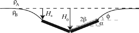
Figure 3: Cross–section of two shallow, touching strips floating at a liquid–fluid interface.

Whilst the scenario considered in the previous section may be relevant in practical situations, it does not lend itself to particularly simple experimental validation. To allow for such a comparison, we now consider the equilibrium of two infinitely long, shallow strips of dimensional thickness $\ell_{c}t$, width $2\ell_{c}\beta$, and density $\rho_{s}$, floating with their long edges in contact so that the interior meniscus is completely eliminated. The configuration is shown schematically in figure 3. Here, we are no longer bound by a contact angle condition but instead assume that the meniscus is pinned to the uppermost corners of the strips. The additional complication of the strip’s angle of inclination to the horizontal, $\alpha$, is determined by the balance of torques. (This condition is satisfied automatically for shapes with circular cross-section and constant contact angle, as shown by Singh & Hesla (2004).)

Equating moments about the point of contact (thereby eliminating the need to calculate the tension force that the strips exert on one another) and balancing vertical forces, we obtain the conditions for equilibrium

$${\cal D}\beta\cos\alpha=\sin(\phi-\alpha)-\beta(H_{0}+\tfrac{4}{3}\beta\sin\alpha),$$ (6)

$${\cal D}\beta=\tfrac{1}{2}\sin\phi-\beta\cos\alpha(H_{0}+\beta\sin\alpha),$$ (7)

where

$${\cal D}\equiv\frac{(\rho_{s}-\rho_{B})t}{\rho_{B}-\rho_{A}}$$ (8)

is the appropriate ratio of the density of the strips to those of the surrounding fluids. After eliminating ${\cal D}$ between (6) and (7) and using (3) with the relation $H_{*}=H_{0}+2\beta\sin\alpha$ to eliminate $\phi$, we have a single equation for $\alpha$ given particular values of $\beta$ and $H_{0}$. Thus, for fixed $\beta$ and a given value of $H_{0}$, we may solve for $\alpha$ and deduce the corresponding value of ${\cal D}$ from (7). By varying $H_{0}$ we are then able to calculate the maximum value of ${\cal D}$ for which equilibrium is possible, much as before. The numerical results of this calculation are presented in figure 4.

\psfrag{labelbeta}{$\beta$}\psfrag{labeld}{${\cal D}$}\includegraphics[height=142.26378pt]{2stripdat4}

Figure 4: Numerically computed values of ${\cal D}_{\mathrm{max}}$ as the half-width of the strips, $\beta$, is varied (solid line). Experimental results (as described in text) are shown by points $\times$ (strips that sink) and $\bigcirc$ (strips that float).

Also shown in figure 4 are experimental results showing points in $(\beta,{\cal D})$ parameter space for which two identical strips remained afloat or sank upon touching. These experiments were performed with strips of stainless-steel shim of length $69\,\mathrm{mm}$ with $\rho_{s}=7905\,\mathrm{kg}\,\mathrm{m}^{-3}$ and thickness $0.4$ or $0.5\,\mathrm{mm}$. These were floated on aqueous solutions of $0\%$, $10\%$ or $25\%$ methanol in air (so that $\rho_{A}\ll\rho_{B}$), allowing a wide range of values of $\beta$ and ${\cal D}$ to be probed. The strips were then allowed to come into contact naturally via the mutually attractive flotation force Mansfield et al. (1997). The data are plotted with horizontal and vertical error bars. The former indicate the uncertainty in the measurement of the strip widths. The latter indicate the uncertainty in the additional vertical force contribution of the ends (since the strips are of finite length), which may be shown to be equivalent to an uncertainty in the effective value of ${\cal D}$. The agreement between our experiments and theory in this instance is very good.

4 The floating of a flexible raft

By adding additional strips to a floating pair of strips, a flexible raft is formed. Given the analysis of the preceding sections it is natural to expect that as the raft is lengthened in this manner, there will come a point where its weight (which scales with its total length) exceeds the force that can be supplied by surface tension (which is constant) and so the raft should sink. The situation is complicated by the fact that the raft may bow in its middle, displacing a considerable amount of liquid in this region, as pointed out by Saif (2002). We now address the question of whether, for a raft of given weight per unit length, there is a maximum raft length before sinking occurs.

We tackle this problem by treating the raft as a continuum, shown schematically in fig. 5, and formulating an equation for the deformation of such a raft. This generalises the linear analysis of Mansfield et al. (1997) and allows us to consider situations in which interfacial deformations are no longer small, including the existence of a threshold length for sinking.

\psfrag{labelbeta}{$\beta$}\psfrag{labeld}{${\cal D}$}\includegraphics[height=71.13188pt]{raftset}

Figure 5: Schematic illustration of a flexible raft floating at an interface.

4.1 Governing equation

We use a variational approach to determine the shape $(X(S),H(S))$ of the raft and the surrounding meniscus, though the same result may also be obtained by considering the force balance on an infinitesimal raft element. The non-dimensional arc-length, $S$, is measured from the raft’s axis of symmetry at $S=0$, with the two ends of the raft being at $S=\pm L$. For simplicity, we neglect the intrinsic bending stiffness of the raft, although Vella, Aussillous & Mahadevan (2004) have shown that interfacial rafts do, in general, have some resistance to bending. The variational principle states that raft shapes must minimise the energy of the system over variations in $H(S)$ and $X(S)$, subject to the constraint that $X_{S}^{2}+H_{S}^{2}=1$. Introducing a Lagrange multiplier $\lambda(S)$ associated with this constraint, we find that equilibrium raft shapes extremise

$${\cal E}\equiv\int_{-\infty}^{\infty}\left(X_{S}(H^{2}/2-1)+{\cal D}H\chi+(1-\chi)+\lambda(S)\bigl{[}(X_{S}^{2}+H_{S}^{2})^{1/2}-1\bigr{]}\right)\mathrm{d}S,$$ (9)

where ${\cal D}$ was defined in (8) and

$$\chi(S)\equiv\begin{cases}1,&|S|\leq L\\ 0,&|S|>L,\end{cases}$$ (10)

is the indicator function of the raft.

The first two terms in the integral (9) correspond to the gravitational energy of the displaced fluid and the raft, the third term is the surface energy of the uncovered liquid area, and the final term ensures that the constraint $X_{S}^{2}+H_{S}^{2}=1$ is satisfied. Note that a small increase in arc-length such that $X_{S}^{2}+H_{S}^{2}>1$ increases the energy of the system so that the Lagrange multiplier $\lambda(S)$ may be interpreted physically as the tension in the raft/meniscus. That the raft can support a tension at all may seem counterintuitive. It is a consequence of the attractive capillary interaction that would exist between two infinitesimally separated raft elements.

Requiring ${\cal E}$ to be stationary with respect to variations in $H(S)$ and $X(S)$ yields differential equations for $X$ and $H$. Using the differential form of the constraint, $X_{S}X_{SS}+H_{S}H_{SS}=0$, we may eliminate $\lambda$ to obtain $\lambda_{S}=\chi{\cal D}H_{S}$. This may be integrated using the boundary term from integration by parts at $\pm\infty$, the boundary conditions $H(\pm\infty)=0$ and $X_{S}(\pm\infty)=1$ as well as the continuity of $\lambda$ at the raft edge, $S=\pm L$, to give $\lambda=1+\chi{\cal D}(H-H_{*})$, where $H_{*}\equiv H(\pm L)$. We now find the raft shape numerically by solving the nonlinear eigenproblem

$$\begin{gathered}X_{S}=\cos\theta,\quad H_{S}=\sin\theta,\quad\theta_{S}=\frac{H+{\cal D}\cos\theta}{1+{\cal D}(H-H_{*})},\\ X(0)=0,\quad\theta(0)=0,\quad\theta(L)=2\arcsin(H_{*}/2),\quad H(L)=H_{*},\end{gathered}$$ (11)

for $X(S)$, $H(S)$, $\theta(S)$ on $[0,L]$, and $H_{*}$, using the MATLAB routine bvp4c. The results of this computation may be verified by calculation of the quantity

$$P(\theta)\equiv\tfrac{1}{2}H^{2}+\bigl{[}1+{\cal D}(H-H_{*})\bigr{]}\cos\theta-1,$$ (12)

which is conserved and, from the boundary conditions, equal to $0$.

In the limit of small deformations (11) reduces to the simpler linear form studied by Mansfield et al. (1997) in the context of determining typical raft profiles. Here, however, we wish to determine whether a maximum raft length, $2L_{\mathrm{max}}$, exists and if so find its value for a raft of given density ${\cal D}$. To investigate this, small deformation theory is inadequate since sinking is an essentially non-linear phenomenon.

The symmetry condition $\theta(0)=0$ ensures that $H_{*}\geq-{\cal D}/2$ and that $H_{0}\equiv H(0)\geq-{\cal D}$, so that the centre of the raft may sink at most to its neutral buoyancy level. In what follows, it will be convenient to treat $H_{0}$ and ${\cal D}$ as parameters giving rise to a particular raft semi-length $L(H_{0},{\cal D})$; we find

$$L(H_{0},{\cal D})=\frac{H_{0}^{2}}{2{\cal D}}\int_{0}^{1}\frac{2+H_{0}^{2}(y-1)}{\Bigl{\{}\bigl{[}2+H_{0}^{2}(y-1)\bigr{]}^{2}-\bigl{[}2-(H_{0}+yH_{0}^{2}/2{\cal D})^{2}\bigr{]}^{2}\Bigr{\}}^{1/2}}\mathrm{d}y,$$ (13)

which follows by changing integration variables from $S$ to $H$ in $L=\int_{0}^{L}\mathrm{d}S$. This allows us to consider the behaviour of $L$ for a given value of ${\cal D}$ as $H_{0}$ is varied.

The tension at the midpoint of the raft is given by $1-H_{0}^{2}/2$, showing that the raft goes into compression if $H_{0}\leq-\sqrt{2}$. Physically this is unrealistic, corresponding to a divergence in $\theta_{S}$. If ${\cal D}<\sqrt{2}$, this situation is avoided automatically since $H_{0}\geq-{\cal D}>-\sqrt{2}$ but for ${\cal D}\geq\sqrt{2}$ we must consider this possibility; we therefore consider these two cases separately.

4.2 The case ${\cal D}<\sqrt{2}$

When ${\cal D}<\sqrt{2}$, the centre of the raft may reach its neutral buoyancy depth $H_{0}=-{\cal D}$ without going into compression. Numerical computation of the integral (13) suggests that rafts grow arbitrarily long as $H_{0}\searrow-{\cal D}$ (see figure 6$a$). To show that this is the case, we consider the asymptotic behaviour of the integral (13) in the limit $\epsilon\equiv{\cal D}+H_{0}\ll 1$. This is done by splitting the range of integration into two sub-regions $[0,\delta]$ and $(\delta,1]$, where $\delta$ is unspecified save for the condition that $\epsilon\ll\delta\ll 1$ (see Hinch, 1990). Within these two regions, the two integrands may be simplified using approximations compatible with this gearing of $\delta$, and the resulting integrals evaluated analytically. Upon expanding these results for $\delta\ll 1$ the leading order terms in $\delta$ cancel, yielding

$$L=-\mu\log\left(\frac{\epsilon}{{\cal D}}\right) + \mu\log\left(\frac{8\mu^{2}}{\sqrt{2}\mu(7+\mu^{2})^{1/2}+4-{\cal D}^{2}}\right)$$ (14)

$$- 2{\cal D}\arctan\left(\frac{{\cal D}(3\mu-\sqrt{2}(7+\mu^{2})^{1/2})}{3{\cal D}^{2}+\sqrt{2}\mu(7+\mu^{2})^{1/2}}\right)+O(\epsilon^{1/2}),$$

where $\mu\equiv(1-{\cal D}^{2}/2)^{1/2}$. This result compares favourably with the numerical results in figure 6(a). In particular, notice that $L$ diverges logarithmically as $H_{0}\searrow-{\cal D}$ (i.e. as $\epsilon\rightarrow 0$) so that rafts of arbitrary length are possible. It also interesting to note that (14) may be inverted to give an estimate of $H_{0}=-{\cal D}+\epsilon$ for given values of ${\cal D}$ and $L$ — a useful result when calculating raft shapes for large $L$.

That a raft of sufficiently low density can grow arbitrarily large in horizontal extent without sinking seems surprising at first glance. However, as new material is added to the raft, it may be accommodated at its neutral buoyancy level without the raft going into compression. Therefore, the raft’s ability to remain afloat is not jeopardised and it is almost obvious that these low density rafts may grow arbitrarily long without sinking.

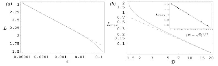
Figure 6: ($a$) Numerical results of the calculation of $L$ as a function of $\epsilon\equiv H_{0}+{\cal D}$ (solid line) compared to the asymptotic result (14) for $\epsilon\ll 1$ (dashed line) for the case ${\cal D}=1.4$. ($b$) Main figure: Numerical results of the calculation of $L_{\mathrm{max}}$ as a function of the density ratio ${\cal D}\geq\sqrt{2}$ (solid line), together with the large ${{\cal D}}$ asymptotic result $L_{\mathrm{max}}\sim 1/{\cal D}$ (dashed line). Inset: Rescaled graph comparing the numerically computed values (points) of $L_{\mathrm{max}}$ with the asymptotic expansion (17) (solid line).

4.3 The case ${\cal D}\geq\sqrt{2}$

In this case, the raft cannot reach its neutral buoyancy level, invalidating the argument just given to explain why, with ${\cal D}<\sqrt{2}$, rafts may be arbitrarily large. We thus expect that a maximum raft length does exist and, further, that the limiting raft has $H_{0}=-\sqrt{2}$. Numerical computation of $L$ as a function of $H_{0}$ indicates that a critical half-length $L_{\mathrm{max}}$ does exist, but that it is not attained with exactly this value of $H_{0}$. Instead, there is a competition between the raft sinking deep into the liquid (to support its weight by increased hydrostatic pressure) and having its ends a large distance apart (i.e. lower pressure but over larger horizontal distances), and some compromise is reached. Given the abrupt change in behaviour observed as ${\cal D}$ increases past $\sqrt{2}$, we are particularly interested in the nature of this transition. Numerical computations suggest that for $\eta^{2}\equiv{\cal D}-\sqrt{2}\ll 1$, $L_{\mathrm{max}}$ occurs when $H_{0}=-\sqrt{2}+c\eta^{2}$ for some constant $c$. Motivated by this observation, we let $H_{0}=-\sqrt{2}+c\eta^{2}$ and again split the domain of integration in (13) into two regions $[0,\delta^{\prime}]$ and $[\delta^{\prime},1]$ where $\eta^{2}\ll\delta^{\prime}\ll 1$. This allows us to calculate $L$ to leading order in $\eta$, yielding

$$L=2\sqrt{2}\arctan\left(\frac{\sqrt{7}}{3}\right)+\eta\frac{2^{3/4}c}{(c+1)^{1/2}}\left[\mathrm{K}\left(\frac{c+2}{2(c+1)}\right)-\frac{2(c+1)}{c}\mathrm{E}\left(\frac{c+2}{2(c+1)}\right)\right]+O(\eta^{2}),$$ (15)

where $\mathrm{K}(k)\equiv\int_{0}^{\pi/2}(1-k^{2}\sin^{2}\phi)^{-1/2}\mathrm{d}\phi$ and $\mathrm{E}(k)\equiv\int_{0}^{\pi/2}(1-k^{2}\sin^{2}\phi)^{1/2}\mathrm{d}\phi$ are the complete elliptic integrals of the first and second kinds, respectively. The coefficient of $\eta$ in (15) has a maximum for fixed $\eta$ at $c=c^{*}$, where $c^{*}$ satisfies

$$\mathrm{K}\left(\frac{c^{*}+2}{2c^{*}+2}\right)=2\mathrm{E}\left(\frac{c^{*}+2}{2c^{*}+2}\right).$$ (16)

Hence $c^{*}\approx 0.5332$, and we obtain the asymptotic expression

$$L_{\mathrm{max}}=2\sqrt{2}\arctan\left(\tfrac{\sqrt{7}}{3}\right)-3.1525\left({\cal D}-\sqrt{2}\right)^{1/2}+O\left({\cal D}-\sqrt{2}\right),$$ (17)

which compares very favourably with the numerically computed values of $L_{\mathrm{max}}$ presented in the inset of figure 6($b$).

For the limiting case ${\cal D}=\sqrt{2}$, the above analysis breaks down since then $\eta=0$ and we lose the freedom to vary $H_{0}$. However, by letting $\epsilon=c\eta^{2}$ (so that $H_{0}=\epsilon-\sqrt{2}$) we take the limit $\eta\rightarrow 0$ of (15) with $\epsilon\ll 1$ fixed to find

$$L(\epsilon)=2\sqrt{2}\arctan\left(\tfrac{\sqrt{7}}{3}\right)+\epsilon^{1/2}2^{3/4}\left[\mathrm{K}(\tfrac{1}{2})-2\mathrm{E}(\tfrac{1}{2})\right]+O(\epsilon).$$ (18)

This has a maximum value of $2\sqrt{2}\arctan(\sqrt{7}/3)$ at $\epsilon=0$, which is the same value as that found from (17) in the limit ${\cal D}\searrow\sqrt{2}$. It is also reassuring to note that, as ${\cal D}\nearrow\sqrt{2}$ with $\epsilon$ fixed, the expression in (14) also gives $L=2\sqrt{2}\arctan(\sqrt{7}/3)+O(\epsilon^{1/2})$.

For completeness, we consider finally the limit ${\cal D}\gg 1$. To leading order in ${\cal D}^{-1}$, the integral for $L(H_{0},{\cal D})$ is given by

$$L(H_{0},{\cal D})\sim{\cal D}^{-1}\int_{1-H_{0}^{2}/2}^{1}\frac{u}{(u^{2}-(1-H_{0}^{2}/2)^{2})^{1/2}}\mathrm{d}u={\cal D}^{-1}H_{0}(1-H_{0}^{2}/4)^{1/2}.$$ (19)

This has a maximum value of ${\cal D}^{-1}$ at $H_{0}=-\sqrt{2}$ so that in the limit ${\cal D}\gg 1$, $L_{\max}\sim{\cal D}^{-1}$. This is precisely as we should expect physically since large density objects can only float when the contribution of surface tension dominates that of the buoyancy due to excluded volume and, in particular, it must balance the weight of the raft. This asymptotic result compares favourably with the the numerical results presented in figure 6($b$).

4.4 Comparison with experiment

A direct comparison between the theoretical results outlined so far and experimental results is difficult since we have modelled the raft as a perfectly flexible continuum body of infinite extent along its axis of symmetry. Despite these limitations, the theoretical raft shapes calculated via this model are in good agreement with simple experiments in which thin strips of stainless steel shim are laid side-by-side at an air–water interface, as shown in figure 7 — even when the raft consists of only a small number of strips and we might not expect the continuum approximation to be valid.

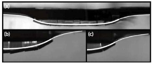
Figure 7: Comparison between experimental realisation of a two-dimensional raft (viewed through the side of a transparent tank) and the theoretically predicted shape (superimposed white line). The rafts float at an air–water interface and have varying values of ${\cal D}$ and $L$: ($a$) a complete raft with ${\cal D}=1.02$, $L=4.03$ ($b$) one half of a raft with ${\cal D}=1.27$, $L=1.47$ and ($c$) one half of a raft with ${\cal D}=1.27$, $L=2.57$. The typical width of each individual strip is $2$ mm. The black region apparently above the raft is in fact a reflection of the black base of the confining tank from the meniscus at the edge of the tank

Although this agreement is encouraging, our main interest lies more in whether there is a maximum length for such a raft to remain afloat, as predicted by the model. Practical considerations mean it is difficult to produce strips of stainless steel shim narrower than about $2$ mm in the workshop, so the comparisons we are able to draw between our model and experiments can only be semi-quantitative. In spite of these limitations, we find that for stainless steel strips of length $69$ mm and thickness $0.5$ mm the maximum raft-length is $4-6$ mm for an aqueous solution of 25% methanol (so that $1.645\geq{\cal D}\geq 1.580$) and $6-8$ mm for 15% methanol (so that $1.494\geq{\cal D}\geq 1.424$), which are certainly consistent with the corresponding theoretical results of $4.6$ mm $\leq L_{\mathrm{max}}\leq 4.8$ mm and $6.5$ mm $\leq L_{\mathrm{max}}\leq 7.2$ mm, respectively. Here the length was increased by floating additional strips near the raft and allowing them to come into contact via the mutually attractive capillary flotation forces until the raft was no longer stable and sank. With ${\cal D}=1.02$ and ${\cal D}=1.27$, we were able to add many strips without any sign of the raft sinking indicating that this process might be continued indefinitely.

5 Discussion

In this article, we have quantified the conditions under which objects can remain trapped at a fluid-fluid interface, and shown that when the deformation of the meniscus is suppressed by the presence of other objects the supporting force that can be generated decreases dramatically. For two small, parallel cylinders or strips, the maximum force that can be supported close to contact is only that provided by the contribution from the exterior meniscus and so sufficiently dense objects sink upon contact. A two-dimensional raft of touching, floating strips may compensate partially for this loss of meniscus by sinking lower into the fluid. For ${\cal D}<\sqrt{2}$, this effect allows rafts of arbitrary length to remain afloat. For ${\cal D}\geq\sqrt{2}$, there is a maximum length (dependent on ${\cal D}$) above which equilibrium is not possible.

Although the agreement between the experiments and theory presented here is good, our analysis was confined to two dimensions, whereas experiments must be carried out in the three-dimensional world. Similarly, we have limited ourselves to considering the equilibrium of objects at an interface. We are currently studying the dynamics of sinking for the case of two touching strips considered in section 3, and find that a simple hydrodynamic model produces good agreement with experiments.