Numerical modeling of quasiplanar giant water waves

Abstract

In this work we present a further analytical development and a numerical implementation of the recently suggested theoretical model for highly nonlinear potential long-crested water waves, where weak three-dimensional effects are included as small corrections to exact two-dimensional equations written in the conformal variables [V.P. Ruban, Phys. Rev. E 71, 055303(R) (2005)]. Numerical experiments based on this theory describe the spontaneous formation of a single weakly three-dimensional large-amplitude wave (alternatively called freak, killer, rogue or giant wave) on the deep water.

I Introduction

Rogue waves are extremely high, steep and dangerous individual waves which sometimes appear suddenly on a sea surface among relatively low waves (see, for instance, the recent works Kharif-Pelinovsky ; ZDV2002 ; DZ2005Pisma , and references therein). The crest of a rogue wave can be three or even more times higher than the crests of neighboring waves. Different physical mechanisms contribute to the rogue wave phenomenon: dispersion enhancement, geometrical focusing, wave-current interaction Kharif-Pelinovsky , but the most important at the final stage is the nonlinear self-focusing mechanism resulting in accumulation of the wave energy and momentum on the scale of a single wavelength DZ2005Pisma . For weakly modulated periodic planar Stokes waves this mechanism leads to the well-known Benjamin-Feir instability Benjamin-Feir ; Zakharov67 , generated by four-wave nonlinear resonant interactions $2\to 2$. This instability is predominantly two-dimensional (2D), and it is dominant for low amplitudes ($h/\lambda\leq 0.09$ where $h$ is the peak-to-trough height and $\lambda$ is the length of the Stokes wave McLean_et_al_1981 ). For larger steepness parameter $h/\lambda$, another, genuinely three-dimensional (3D), instability becomes dominant, which is generated by five-wave interactions $3\to 2$, and results in the well-known crescent, or “horse-shoe” wave patterns (see SBK1996 ; Collard-Caulliez-1999 ; Dias-Kharif , and references therein). It is important that real ocean giant waves are observed in situations when this 3D instability is not principal, and all the waves are typically long-crested, corresponding to a narrow-angle Fourier spectrum. Thus, many essential features of a rogue wave formation can be observed already in purely 2D geometry, as in the works by Zakharov and co-workers ZDV2002 ; DZ2005Pisma . For instance, in Ref. DZ2005Pisma a numerical giant wave was computed with the impressive spatial resolution of up to $2\cdot 10^{6}$ points. Zakharov and co-workers simulated an exact system of dynamic equations for 2D free-surface inviscid potential flows, written in terms of the so called conformal variables, which make the free boundary effectively flat (the corresponding exact 2D theory is described in Refs. DKSZ96 ; DZK96 ; ZD96 ; DLZ95 ; Lvov97 ; D2001 ; CC99 ). With these variables, highly nonlinear equations of motion for planar water waves are represented in an exact and compact form containing integral operators diagonal in the Fourier representation. Such integro-differential equations are easy to treat numerically with modern libraries for the discrete fast Fourier transform (FFT) as, for example, FFTW fftw3 . Recently, by introducing an additional conformal mapping, the exact 2D conformal description has been generalized to non-uniform and time-dependent bottom profiles, so that a very accurate 2D modeling of near-coastal waves and tsunami-like processes has been possible R2004PRE ; R2005PLA .

However, real sea waves are never ideally planar, and the second horizontal dimension might play an important role in the wave dynamics. Various numerical methods have been developed for nonlinear 3D surface gravity waves (see TY1996ARFM ; Dias-Kharif ; Dias-Bridges for a review). Some of them are based on exact formulation of the problem (the boundary integral method and its modifications; see L-H_C-1976 ; Clamond-Grue-2001 ; Fructus_et_al_2005 and references therein), another approach uses approximate equations of motion, as the Boussinesq-type models Kirby ; BinghamAgnon , the equations derived by Matsuno Matsuno , by Choi Choi95 , the weakly nonlinear Zakharov equations OOSRPZB2002 ; DKZ2004 , or the equations for wave packets — the nonlinear Schroedinger equation (NLS) and its extensions Dysthe1979 ; TKDV2000 ; OOS2000 ; Janssen2003 . The numerical methods based on exact equations are quite “expensive” and thus provide a relatively low spatial resolution (typically $128\times 64$, as in the recent work Fructus_et_al_2005 for essentially 3D waves). On the other hand, the applicability of the approximate equations is limited by the condition that the waves must not be too steep. To fill this gap, some new approximate, relatively compact explicit equations of motion for highly nonlinear 3D waves were needed as the basis for a new numerical method. Recently, as an extension of the exact conformal 2D theory, a weakly 3D conformal theory has been suggested R2005PRE , which is valid for steep long-crested waves. Equations of this theory contain 3D corrections of the order of $\epsilon=(l_{x}/l_{q})^{2}$, where $l_{x}$ is a typical wave length, and $l_{q}$ is a large transversal scale along the wave crests. In Ref. R2005PRE , the general case was considered, with a static nonuniform quasi-one-dimensional bottom profile. Since the corresponding general equations are rather involved, it is natural to focus on some simple particular cases in the first place, for instance on the deep water limit. The purpose of the present work is a further development of the weakly 3D conformal theory and its numerical implementation for the most simple deep water case. Our main result here is that we have developed a numerical scheme based on FFT which is sufficiently simple, accurate and fast simultaneously. As an application, we have simulated a freak wave formation with the final resolution up to $16384\times 256$.

This article is organized as follows. In Sec. II we adopt for the deep water limit the general weaky 3D fully nonlinear theory described in Ref. R2005PRE . We also suggest some modification of the obtained dynamical system which results in the correct linear dispersion relation not only within a small region near the $k_{1}$-axis, but in the whole Fourier-plane. In Sec. III we describe our numerical method and present numerical results for the problem of a rogue wave formation. Finally, Sec. IV contains our summary and discussion.

II Weakly 3D nonlinear theory

II.1 General remarks

It is a well known fact that a principal difficulty in the 3D theory of potential water waves is the general impossibility to solve exactly the Laplace equation for the velocity potential $\varphi(x,y,q,t)$,

$$\varphi_{xx}+\varphi_{yy}+\varphi_{qq}=0,$$ (1)

in the flow region $-\infty\leq y\leq\eta(x,q,t)$, with the given boundary conditions

$$\varphi|_{y=\eta(x,q,t)}=\psi(x,q,t),\quad\varphi|_{y=-\infty}=0.$$ (2)

(Here $x$ and $q$ are the horizontal Cartesian coordinates, $y$ is the vertical coordinate, while the symbol $z$ will be used for the complex combination $z=x+iy$). Therefore a compact expression is absent for the Hamiltonian functional of the system,

$${\cal H}\{\eta,\psi\} = \frac{1}{2}\int dx\,dq\int\limits_{-\infty}^{\eta(x,q,t)}(\varphi_{x}^{2}+\varphi_{y}^{2}+\varphi_{q}^{2})dy$$ (3)

$$+\frac{g}{2}\int\eta^{2}dx\,dq\equiv{\cal K}\{\eta,\psi\}+{\cal P}\{\eta\},$$

(the sum of the kinetic energy of the fluid and the potential energy in the vertical gravitational field $g$). The Hamiltonian determines canonical equations of motion (see Z1999 ; RR2003PRE ; DKZ2004 , and references therein)

$$\eta_{t}=({\delta{\cal H}}/{\delta\psi}),\qquad-\psi_{t}=({\delta{\cal H}}/{\delta\eta})$$ (4)

in accordance with the variational principle $\delta\int\tilde{\cal L}dt=0$, where the Lagrangian is $\tilde{\cal L}=\int\psi\eta_{t}\,dx\,dq-{\cal H}.$

In the traditional approach, the problem is partly solved by an asymptotic expansion of the kinetic energy ${\cal K}$ on a small parameter — the steepness of the surface (see Refs. Z1999 ; DKZ2004 ; LZ2004 , and references therein). As the result, a weakly nonlinear theory is generated, which is not good to describe large-amplitude steep waves [see Ref. LZ2004 for a discussion about the limits of such theory; practically, the wave steepness $ka$ ($k$ is a wave number, $a$ is an amplitude) should be not more than $0.1$ (that is $h/\lambda\leq 0.1/\pi\approx 0.03$)]. Below in this section we consider a different, recently developed theory R2005PRE (adopted here for the case of infinite depth), which is based on another small parameter — the ratio of a typical length of the waves propagating along the $x$-axis, to a large scale along the transversal horizontal direction, denoted by $q$ [alternatively, it is the ratio of typical wave numbers $k_{q}/k_{x}$ in the Fourier plane $(k_{x},k_{q})$]. Thus, we define $\epsilon=(l_{x}/l_{q})^{2}\ll 1$ and note: the less this parameter, the less our flow differs from a purely 2D flow, and the more accurate the equations are. A profile $y=\eta(x,q,t)$ of the free surface and a boundary value of the velocity potential $\psi(x,q,t)\equiv\varphi(x,\eta(x,q,t),q,t)$ are allowed to depend strongly on the coordinate $x$, while the derivatives over the coordinate $q$ will be small: $|\eta_{q}|\sim\epsilon^{1/2}$, $|\psi_{q}|\sim\epsilon^{1/2}$.

II.2 Conformal variables in 3D

In the same manner as in the exact 2D theory DKSZ96 ; DLZ95 , instead of the Cartesian coordinates $x$ and $y$, we use curvilinear conformal coordinates $u$ and $v$, which make the free surface effectively flat:

$$x+iy\equiv z=z(u+iv,q,t),\quad-\infty\leq v\leq 0,$$ (5)

where $z(w,q,t)$ is an analytical on the complex variable $w\equiv u+iv$ function without any singularities in the lower half-plane $-\infty\leq v\leq 0$. The profile of the free surface is now given in a parametric form by the formula

$$X(u,q,t)+iY(u,q,t)\equiv Z(u,q,t)=z(u+0i,q,t).$$ (6)

Here the real functions $X(u,q,t)$ and $Y(u,q,t)$ are related to each other by the Hilbert transform $\hat{H}$:

$$X(u,q,t)=u-\hat{H}Y(u,q,t).$$ (7)

The Hilbert operator $\hat{H}$ is diagonal in the Fourier representation: it multiplies the Fourier-harmonics $Y_{k}(q,t)\equiv\int Y(u,q,t)e^{-iku}du$ by $i\,\mbox{sign\,}k$, so that

$$\hat{H}Y(u,q,t)=\int[i\,\mbox{sign\,}k]Y_{k}(q,t)e^{iku}({dk}/{2\pi}).$$ (8)

The boundary value of the velocity potential is $\varphi|_{v=0}\equiv\psi(u,q,t)$.

For equations to be shorter, below we do not indicate the arguments $(u,q,t)$ of the functions $\psi$, $Z$ and $\bar{Z}$ (the overline denotes complex conjugate). The Lagrangian for 3D deep water waves in terms of the variables $\psi$, $Z$, and $\bar{Z}$ can be written as follows (compare with R2005PRE ):

$${\cal L} = \int\left[\frac{Z_{t}\bar{Z}_{u}-\bar{Z}_{t}Z_{u}}{2i}\right]\psi\,du\,dq-{\cal K}\{\psi,Z,\bar{Z}\}$$

$$- \frac{g}{2}\int\left[\frac{Z-\bar{Z}}{2i}\right]^{2}\left[\frac{Z_{u}+\bar{Z}_{u}}{2}\right]du\,dq$$

$$+ \int\Lambda\left[\hat{H}\left(\frac{Z-\bar{Z}}{2i}\right)+\left(\frac{Z+\bar{Z}}{2}-u\right)\right]du\,dq,$$ (9)

where the indefinite real Lagrangian multiplier $\Lambda(u,q,t)$ has been introduced in order to take into account the relation (7). Equations of motion follow from the variational principle $\delta{\cal A}=0$, with the action ${\cal A}\equiv\int{\cal L}dt$. So, variation by $\delta\psi$ gives us the first equation of motion — the kinematic condition on the free surface

$$\mbox{Im\,}(Z_{t}\bar{Z}_{u})=({\delta{\cal K}}/{\delta\psi}).$$ (10)

Let us divide this equation by $|Z_{u}|^{2}$ and use analytical properties of the function $Z_{t}/Z_{u}$. As a result, we obtain the time-derivative-resolved equation

$$Z_{t}=iZ_{u}(1+i\hat{H})\left[\frac{(\delta{\cal K}/\delta\psi)}{|Z_{u}|^{2}}\right].$$ (11)

Further, variation of the action ${\cal A}$ by $\delta Z$ gives us the second equation of motion:

$$\left[\frac{\psi_{u}\bar{Z}_{t}-\psi_{t}\bar{Z}_{u}}{2i}\right]=\left(\frac{\delta{\cal K}}{\delta Z}\right)+\frac{g}{2i}\,\mbox{Im}\Big{(}Z\Big{)}\bar{Z}_{u}-\frac{(\hat{H}-i)\Lambda}{2i}.$$ (12)

After multiplying Eq.(12) by $-2iZ_{u}$ we have

$$[\psi_{t}+g\,\mbox{Im\,}Z]|Z_{u}|^{2}-\psi_{u}\bar{Z}_{t}Z_{u}=(i-\hat{H})\tilde{\Lambda}-2i\left(\frac{\delta{\cal K}}{\delta Z}\right)Z_{u},$$ (13)

where $\tilde{\Lambda}$ is another real function. Taking the imaginary part of Eq.(13) and using Eq.(10), we find $\tilde{\Lambda}$:

$$\tilde{\Lambda}=\left[\psi_{u}\frac{\delta{\cal K}}{\delta\psi}\right]+2\,\mbox{Re}\left[\left(\frac{\delta{\cal K}}{\delta Z}\right)Z_{u}\right].$$ (14)

After that, the real part of Eq.(13) gives us the Bernoulli equation in a general form:

$$\psi_{t} = -g\,\mbox{Im\,}Z-\psi_{u}\hat{H}\left[\frac{(\delta{\cal K}/\delta\psi)}{|Z_{u}|^{2}}\right]$$

$$+ \frac{\mbox{Im}\left((1-i\hat{H})\left[2({\delta{\cal K}}/{\delta Z})Z_{u}+({\delta{\cal K}}/{\delta\psi})\psi_{u}\right]\right)}{|Z_{u}|^{2}}.$$ (15)

Equations (11) and (15) completely determine evolution of the system, provided the kinetic energy functional ${\cal K}\{\psi,Z,\bar{Z}\}$ is explicitly given. It should be emphasized that in our description a general expression for ${\cal K}$ remains unknown. However, under the conditions $|z_{q}|\ll 1$, $|\varphi_{q}|\ll 1$, the potential $\varphi(u,v,q,t)$ is efficiently expanded into a series on the powers of the small parameter $\epsilon$:

$$\varphi=\varphi^{(0)}+\varphi^{(1)}+\varphi^{(2)}+\dots,\qquad\varphi^{(n)}\sim\epsilon^{n},$$ (16)

where $\varphi^{(n+1)}$ can be calculated from $\varphi^{(n)}$, and the zeroth-order term $\varphi^{(0)}=\mbox{Re\,}\phi(w,q,t)$ is the real part of an easily represented (in integral form) analytical function with the boundary condition $\mbox{Re\,}\phi|_{v=0}=\psi(u,q,t)$. Correspondingly, the kinetic energy functional will be written in the form

$${\cal K}={\cal K}^{(0)}+{\cal K}^{(1)}+\dots,\qquad{\cal K}^{(n)}\sim\epsilon^{n},$$ (17)

where ${\cal K}^{(0)}\{\psi\}$ is the kinetic energy of a purely 2D flow,

$${\cal K}^{(0)}\{\psi\} = \frac{1}{2}\int[(\varphi^{(0)}_{u})^{2}+(\varphi^{(0)}_{v})^{2}]\,du\,dv\,dq$$ (18)

$$= -\frac{1}{2}\int\psi\hat{H}\psi_{u}\,du\,dq,$$

and the other terms are corrections due to gradients along $q$. Now we are going to calculate a first-order correction ${\cal K}^{(1)}$.

II.3 First-order corrections

As a result of the conformal change of two variables, the kinetic energy functional is determined by the expression

$${\cal K}=\frac{1}{2}\int\left[\varphi_{u}^{2}+\varphi_{v}^{2}+J({\bf Q}\cdot\nabla\varphi)^{2}\right]du\,dv\,dq,$$ (19)

where the Cauchy-Riemann conditions $x_{u}=y_{v}$, $x_{v}=-y_{u}$ have been taken into account, and the following notations are used:

$$J\equiv|z_{u}|^{2},\qquad({\bf Q}\cdot\nabla\varphi)\equiv a\varphi_{u}+b\varphi_{v}+\varphi_{q},$$

$$a=\frac{x_{v}y_{q}-x_{q}y_{v}}{J}\sim\epsilon^{1/2},\quad b=\frac{y_{u}x_{q}-y_{q}x_{u}}{J}\sim\epsilon^{1/2}.$$

Consequently, the Laplace equation in the new coordinates takes the form

$$\varphi_{uu}+\varphi_{vv}+\nabla\cdot({\bf Q}J({\bf Q}\cdot\nabla\varphi))=0,$$ (20)

with the boundary conditions

$$\varphi|_{v=0}=\psi(u,q,t),\quad\varphi|_{v=-\infty}=0.$$ (21)

In the limit $\epsilon\ll 1$ it is possible to write the solution as the series (16), with the zeroth-order term satisfying the 2D Laplace equation $\varphi_{uu}^{(0)}+\varphi_{vv}^{(0)}=0,$ $\varphi|^{(0)}_{v=0}=\psi(u,q,t)$. Thus, it can be represented as $\varphi^{(0)}=\mbox{Re\,}\phi(w,q,t)$, where

$$\phi(w,q,t)=\int_{-\infty}^{+\infty}(1-\mbox{sign\,}k)\psi_{k}(q,t)e^{ikw}\frac{dk}{2\pi},$$ (22)

and $\psi_{k}(q,t)\equiv\int\psi(u,q,t)e^{-iku}du.$ On the free surface

$$\phi(u+i0,q,t)\equiv\Psi(u,q,t)=(1+i\hat{H})\psi(u,q,t).$$ (23)

For all the other terms in Eq.(16) we have the relations

$$\varphi_{uu}^{(n+1)}+\varphi_{vv}^{(n+1)}+\nabla\cdot({\bf Q}J({\bf Q}\cdot\nabla\varphi^{(n)}))=0$$ (24)

and the boundary conditions $\varphi^{(n+1)}|_{v=0}=0$. Noting that $\int(\varphi_{u}^{(0)}\varphi_{u}^{(1)}+\varphi_{v}^{(0)}\varphi_{v}^{(1)})\,du\,dv=0$ (it is easily seen without explicit calculation of $\varphi^{(1)}$ after integration by parts), we have in the first approximation

$${\cal K}^{(1)} = \frac{1}{2}\int J(\varphi_{q}^{(0)}+a\varphi_{u}^{(0)}+b\varphi_{v}^{(0)})^{2}du\,dv\,dq$$ (25)

$$= \frac{1}{2}\int z_{u}\bar{z}_{u}\left[\mbox{Re}\left(\phi_{q}-\frac{\phi_{u}z_{q}}{z_{u}}\right)\right]^{2}du\,dv\,dq.$$

Since $z(w)$ and $\phi(w)$ are represented as $z(u+iv)=e^{-\hat{k}v}Z(u)$ and $\phi(u+iv)=e^{-\hat{k}v}\Psi(u)$, we can use for $v$-integration the following auxiliary formulas:

$$\!\int du\int_{-\infty}^{0}[e^{-\hat{k}v}A(u)]\overline{[e^{-\hat{k}v}B(u)]}\,dv\!=-\int_{-\infty}^{0}\frac{A_{k}\overline{B_{k}}}{2k}\frac{dk}{2\pi}$$

$$\!=-\frac{i}{2}\!\int\!\left(\overline{B(u)}\,\hat{\partial}_{u}^{-1}\!A(u)\right)du.$$ (26)

Now we apply the above formulas to appropriately decomposed Eq.(25) and, as a result, we obtain an expression of a form ${\cal K}^{(1)}={\cal F}\{\Psi,\overline{\Psi},Z,\overline{Z}\}$, where the functional ${\cal F}$ is defined as follows (compare with R2005PRE )

$$\!\!{\cal F}\!\! = \!\frac{i}{8}\int(Z_{u}\Psi_{q}-Z_{q}\Psi_{u})\hat{\partial}_{u}^{-1}\overline{(Z_{u}\Psi_{q}-Z_{q}\Psi_{u})}\,du\,dq$$ (27)

$$+ \frac{i}{16}\int\!\Bigg{\{}\!\!\left[(Z_{u}\Psi_{q}-Z_{q}\Psi_{u})^{2}/{Z_{u}}\right]\overline{(Z-u)}$$

$$\qquad-(Z-u)\,\overline{\left[(Z_{u}\Psi_{q}-Z_{q}\Psi_{u})^{2}/{Z_{u}}\right]}\!\Bigg{\}}\,du\,dq.$$

Here the combination $(Z-u)$ is written instead of $Z$ just for convenience, as it is finite at the infinity. Actually the equations of motion “do not feel” this difference. In the derivation we have used the identity $\int[(Z_{u}\Psi_{q}-Z_{q}\Psi_{u})^{2}/{Z_{u}}]udu=0$, which holds because the integrand is analytical in the lower half-plane. From here one can express the variational derivatives $(\delta{\cal K}^{(1)}/{\delta\psi})$ and $(\delta{\cal K}^{(1)}/{\delta Z})$ by the formulas

$$\frac{\delta{\cal K}^{(1)}}{\delta\psi}=2\,\mbox{Re\,}\left[(1-i\hat{H})\frac{\delta{\cal F}}{\delta\Psi}\right],\qquad\frac{\delta{\cal K}^{(1)}}{\delta Z}=\frac{\delta{\cal F}}{\delta Z}.$$ (28)

The derivatives $(\delta{\cal F}/{\delta\Psi})$ and $(\delta{\cal F}/{\delta Z})$ are calculated in a standard manner:

$$\frac{\delta{\cal F}}{\delta\Psi} = \frac{i}{8}Z_{q}\Big{[}\overline{(Z_{u}\Psi_{q}-Z_{q}\Psi_{u})}$$ (29)

$$\qquad\qquad+\hat{\partial}_{u}[(\Psi_{q}-Z_{q}\Psi_{u}/{Z_{u}})\overline{(Z-u)}]\Big{]}$$

$$-\frac{i}{8}\,Z_{u}\,\hat{\partial}_{q}\Big{[}\hat{\partial}_{u}^{-1}\overline{(Z_{u}\Psi_{q}-Z_{q}\Psi_{u})}$$

$$\qquad\qquad+(\Psi_{q}-Z_{q}\Psi_{u}/{Z_{u}})\overline{(Z-u)}\Big{]},$$

$$\frac{\delta{\cal F}}{\delta Z} = -\frac{i}{8}\Psi_{q}\Big{[}\overline{(Z_{u}\Psi_{q}-Z_{q}\Psi_{u})}$$ (30)

$$\qquad\qquad+\hat{\partial}_{u}[(\Psi_{q}-Z_{q}\Psi_{u}/{Z_{u}})\overline{(Z-u)}]\Big{]}$$

$$+\frac{i}{8}\,\Psi_{u}\,\hat{\partial}_{q}\Big{[}\hat{\partial}_{u}^{-1}\overline{(Z_{u}\Psi_{q}-Z_{q}\Psi_{u})}$$

$$\qquad\qquad+(\Psi_{q}-Z_{q}\Psi_{u}/{Z_{u}})\overline{(Z-u)}\Big{]}$$

$$+\frac{i}{16}\,\Big{[}\hat{\partial}_{u}[(\Psi_{q}-Z_{q}\Psi_{u}/Z_{u})^{2}\overline{(Z-u)}]$$

$$\qquad\qquad-\overline{(\Psi_{q}-Z_{q}\Psi_{u}/{Z_{u}})^{2}{Z_{u}}}\Big{]}.$$

Now one can substitute $(\delta{\cal K}/\delta\psi)\approx-\hat{H}\psi_{u}+(\delta{\cal K}^{(1)}/\delta\psi)$ and $(\delta{\cal K}/\delta Z)\approx(\delta{\cal K}^{(1)}/\delta Z)$ into the equations of motion (11) and (15). Thus, the required weakly 3D equations for deep water waves are completely derived:

$$Z=u+(i-\hat{H})Y(u,q,t),\quad Z_{u}=1+(i-\hat{H})Y_{u}.$$ (31)

$$Z_{t}=-iZ_{u}(1+i\hat{H})\left[{[\hat{H}\psi_{u}-(\delta{\cal K}^{(1)}/\delta\psi)]}/{|Z_{u}|^{2}}\right],$$ (32)

$$\psi_{t}\!\! = \!-g\,Y+\,\psi_{u}\hat{H}\left[{[\hat{H}\psi_{u}-(\delta{\cal K}^{(1)}/\delta\psi)]}/{|Z_{u}|^{2}}\right]$$ (33)

$$+ \!{\hat{H}\left[\psi_{u}[\hat{H}\psi_{u}-(\delta{\cal K}^{(1)}/{\delta\psi})]\right]}/{|Z_{u}|^{2}}$$

$$- \!{2\,\mbox{Re}\left((\hat{H}+i)[Z_{u}({\delta{\cal K}^{(1)}}/{\delta Z})]\right)}/{|Z_{u}|^{2}}.$$

II.4 Modification of the Hamiltonian

It can be easily obtained that the linear dispersion relation for the system (27)-(33) is

$$\omega^{2}(k,m)=g|k|\left(1+\frac{1}{2}\frac{m^{2}}{k^{2}}\right),$$ (34)

where $m$ is the wave-number in the $q$-direction (the wave-number $k$ in the $u$-direction was introduced earlier). Obviously, here we have the first two terms from the expansion of the exact 3D linear dispersion relation

$$\omega^{2}(k,m)=g\sqrt{k^{2}+m^{2}}$$ (35)

on the powers of $m^{2}/k^{2}\ll 1$. Thus, the system (27)-(33) has a non-physical singularity in the dispersion relation near the $m$-axis in the Fourier plane $(k,m)$, where $k/m\to 0$. Therefore, for convenience of the numerical modeling, some regularization could be useful in the approximate Hamiltonian ${\cal K}^{(0)}+{\cal K}^{(1)}+{\cal P}$, where ${\cal P}$ is the potential energy,

$${\cal P}=\frac{g}{2}\int\left[\frac{Z-\bar{Z}}{2i}\right]^{2}\left[\frac{Z_{u}+\bar{Z}_{u}}{2}\right]du\,dq.$$ (36)

Also, the correct linear dispersion relation is strongly desirable, since it determines which waves interact by nonlinear resonances. Of course, a possible regularization is not unique as we keep only zeroth- and first-order terms on $\epsilon=(m/k)^{2}$ in the Hamiltonian. Below we suggest a modification which adds terms of the order ${\cal O}(\epsilon^{2})$ to the approximate Hamiltonian ${\cal P}+{\cal K}^{(0)}+{\cal K}^{(1)}$ (a modified Hamiltonian $\tilde{\cal H}={\cal P}+\tilde{\cal K}$ will remain valid up to $\epsilon$). First of all, instead of the the functional ${\cal K}^{(0)}$ we use another functional, ${\cal K}^{(0)}\to(1/2)\int\psi\hat{G}_{0}\psi\,du\,dq$, where the linear operator $\hat{G}_{0}$ is diagonal in the Fourier representation:

$$G_{0}(k,m)=\sqrt{k^{2}+m^{2}}-\frac{1}{2}\frac{|k|m^{2}}{k^{2}+m^{2}}.$$ (37)

Besides that, we change the operator $i\hat{\partial}_{u}^{-1}=1/k$ in the first line of Eq. (27) by the operator $k/(k^{2}+m^{2})=i\hat{\partial}_{u}\Delta_{2}^{-1}$, which is less singular. As the result, we have the modified approximate kinetic-energy functional in the form

$$\tilde{\cal K}=\frac{1}{2}\int\psi\hat{G}_{0}\psi\,du\,dq+\tilde{\cal F},$$ (38)

$$\tilde{\cal F} = \frac{i}{8}\int(Z_{u}\Psi_{q}-Z_{q}\Psi_{u})\hat{\partial}_{u}\Delta_{2}^{-1}\overline{(Z_{u}\Psi_{q}-Z_{q}\Psi_{u})}\,du\,dq$$ (39)

$$+ \frac{i}{16}\int\Bigg{\{}\left[(Z_{u}\Psi_{q}-Z_{q}\Psi_{u})^{2}/{Z_{u}}\right]\overline{(Z-u)}$$

$$\qquad-(Z-u)\,\overline{\left[(Z_{u}\Psi_{q}-Z_{q}\Psi_{u})^{2}/{Z_{u}}\right]}\Bigg{\}}\,du\,dq.$$

The linear dispersion relation resulting from $\tilde{\cal K}$ is correct in the whole Fourier plane. Besides that, the zeroth- and the first-order terms on $\epsilon$ in $\tilde{\cal K}$ are the same as in ${\cal K}^{(0)}+{\cal K}^{(1)}$. The system of equations, corresponding to the modified Hamiltonian $\tilde{\cal H}$, consists of Eq. (31) and the following equations:

$$Z_{t}=iZ_{u}(1+i\hat{H})\left[{(\delta\tilde{\cal K}/\delta\psi)}/{|Z_{u}|^{2}}\right],$$ (40)

$$\psi_{t} = {\mbox{Im}\left((1-i\hat{H})[2({\delta\tilde{\cal F}}/{\delta Z})Z_{u}+(\delta\tilde{\cal K}/\delta\psi)\psi_{u}]\right)}/{|Z_{u}|^{2}}$$ (41)

$$- g\,Y-\psi_{u}\hat{H}\left[(\delta\tilde{\cal K}/\delta\psi)/|Z_{u}|^{2}\right],$$

$$\frac{\delta\tilde{\cal K}}{\delta\psi}=\hat{G}_{0}\psi+2\,\mbox{Re\,}\left[(1-i\hat{H})\frac{\delta\tilde{\cal F}}{\delta\Psi}\right],$$ (42)

$$\frac{\delta\tilde{\cal F}}{\delta\Psi} = \frac{i}{8}Z_{q}\hat{\partial}_{u}\Big{[}\hat{\partial}_{u}\Delta_{2}^{-1}\overline{(Z_{u}\Psi_{q}-Z_{q}\Psi_{u})}$$ (43)

$$\qquad\qquad+(\Psi_{q}-Z_{q}\Psi_{u}/{Z_{u}})\overline{(Z-u)}\Big{]}$$

$$-\frac{i}{8}\,Z_{u}\,\hat{\partial}_{q}\Big{[}\hat{\partial}_{u}\Delta_{2}^{-1}\overline{(Z_{u}\Psi_{q}-Z_{q}\Psi_{u})}$$

$$\qquad\qquad+(\Psi_{q}-Z_{q}\Psi_{u}/{Z_{u}})\overline{(Z-u)}\Big{]},$$

$$\frac{\delta\tilde{\cal F}}{\delta Z} = -\frac{i}{8}\Psi_{q}\hat{\partial}_{u}\Big{[}\hat{\partial}_{u}\Delta_{2}^{-1}\overline{(Z_{u}\Psi_{q}-Z_{q}\Psi_{u})}$$ (44)

$$\qquad\qquad+(\Psi_{q}-Z_{q}\Psi_{u}/{Z_{u}})\overline{(Z-u)}\Big{]}$$

$$+\frac{i}{8}\,\Psi_{u}\,\hat{\partial}_{q}\Big{[}\hat{\partial}_{u}\Delta_{2}^{-1}\overline{(Z_{u}\Psi_{q}-Z_{q}\Psi_{u})}$$

$$\qquad\qquad+(\Psi_{q}-Z_{q}\Psi_{u}/{Z_{u}})\overline{(Z-u)}\Big{]}$$

$$+\frac{i}{16}\,\Big{[}\hat{\partial}_{u}[(\Psi_{q}-Z_{q}\Psi_{u}/Z_{u})^{2}\overline{(Z-u)}]$$

$$\qquad\qquad\qquad-\overline{(\Psi_{q}-Z_{q}\Psi_{u}/{Z_{u}})^{2}{Z_{u}}}\Big{]}.$$

These equations were integrated numerically as described in the following section. It is interesting to note that we also considered another choice for the regularization, with $G_{0}=(k^{2}+m^{2}/2)(k^{2}+m^{2})^{-1/2}$ instead of $|k|$ in ${\cal K}^{(0)}$, and $(k^{2}+m^{2})^{-1/2}$ instead of $1/|k|$ in the first term in ${\cal K}^{(1)}$. The numerical results were found very close in both cases, since the wave spectra were concentrated in the region $m^{2}/k^{2}\ll 1$.

III Numerical method and results

In our numerical simulations, we used the following procedure. A rectangular domain $L_{u}\times L_{q}$ with the periodic boundary conditions in the $(u,q)$-plane was reduced to the standard dimensionless size $2\pi\times 2\pi$ [the aspect ratio $\varepsilon=(L_{u}/L_{q})^{2}$ was taken into account]. This standard square was discretized by $N\times L$ points $(u_{n},q_{l})=2\pi(n/N,l/L)$, with integer $n$ and $l$. The time variable was rescaled to give $g=1$. As the primary dynamical variables, the (complex) Fourier components $Y_{km}$ and $P_{km}=(k^{2}+\varepsilon m^{2})^{1/4}\psi_{km}$ were used, where $k$ and $m$ were integer numbers in the limits $0\leq k<K$, $-M\leq m\leq M$, with $K\approx 3N/8$, $M\approx 3L/8$. For negative $k$, the properties $Y_{-k,-m}=\overline{Y_{km}}$ and $P_{-k,-m}=\overline{P_{km}}$ were implied. It should be noted that after rescaling $u$, $q$, and $t$, the linear dispersion relation has been $\omega_{km}=(k^{2}+\varepsilon m^{2})^{1/4}$, and that the combinations

$$a_{km}=\frac{Y_{km}+iP_{km}}{\sqrt{2\omega_{km}}}$$

in the linear limit coincide with the normal complex variables DLZ95 ; Z1999 .

Using the FFTW library fftw3 , the quantities $Z(u_{n},q_{l})$, $\Psi(u_{n},q_{l})$, their corresponding $u$- and $q$-derivatives, and $\hat{G}_{0}\psi(u_{n},q_{l})$ are represented by 2-dimensional complex arrays. The variational derivatives (43), (44), (42) and the right-hand-sides of Eqs. (40)-(41) are then computed and transformed into Fourier space in order to evaluate the multi-dimensional function which determines the time derivatives of $Y_{km}$ and $P_{km}$. This function is used in the standard fourth-order Runge-Kutta procedure (RK4) for the time integration of the system. After each RK4 step, a large-wave-number filtering of the arrays $Y_{km}$ and $P_{km}$ is carried out, so that only the Fourier components with $0\leq k<K_{eff}$, $-M_{eff}\leq m\leq M_{eff}$ are kept, where $K_{eff}\approx N/4$ and $M_{eff}\approx L/4$. To estimate the accuracy of the computations, conservation of the total energy $\tilde{\cal H}$ and the mean surface elevation are monitored.

Typically, at $t=0$ we put $N=2^{12}$, $L=2^{6}$, and the initial time step $\tau=0.01$. During the computation, as wave crests become more sharp and the spectra get broadened, we several times adaptively double $N$ (together with $K$, $K_{eff}$) and $L$ (together with $M$, $M_{eff}$), with the time step half-decreasing when $N$ is doubled. At the end, when a giant wave is formed, we have $N=2^{13-14}$, $L=2^{7-8}$. As a result of such adaptive scheme, the conservation of the total energy is kept up to 5-6 decimal digits during most part of the evolution. Only at a very late stage, when $N$ and $L$ are not allowed to double anymore, the conservation is just up to 3-4 digits, and the filtering of the higher harmonics becomes more influential.

The efficiency of the above described numerical method crucially depends on the speed of the FFT routine, since most of the computational time (approximately 80%) is spent in the Fourier transforms. To compute the evolution through the unit (dimensionless) time period, on a modern PC (Intel Pentium IV 3.2 GHz) it takes three-four minutes with $N=4096$, $L=64$, $\tau=0.01$, and more than one hour with $N=8192$, $L=256$, $\tau=0.005$. The total time needed for a single numerical rogue-wave experiment is about 3-5 days.

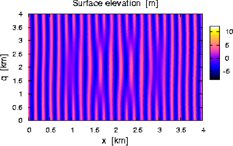
Figure 1: (Color online) [A]. Map of the free surface at $t=0$.

Figure 2: [A]. Initial wave profiles for eight equidistant values $q=L_{q}(0,1/8,\dots,7/8)$.

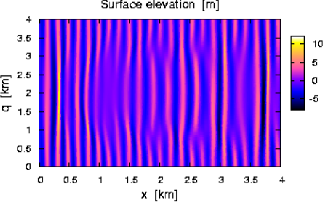
Figure 3: (Color online) [A]. Map of the free surface at $t=59.2$ (the physical time is 7 min 57 sec).

Figure 4: [A]. Wave profiles at $t=59.2$.

Two numerical experiments are reported below for horizontal physical box sizes of $4\times 4$ km (the final resolution was $16384\times 256$ in both). In the first of them, the main mechanism for a big wave formation is the linear dispersion, when a group of longer waves overtakes a group of shorter waves, and their amplitudes are added (see Kharif-Pelinovsky for a discussion). However, due to nonlinear effects, in maximum the crest is higher than simply the sum of two amplitudes. In the second experiment, a giant wave is formed by an essentially nonlinear mechanism (due to Benjamin-Feir instability) from a slightly modulated periodic wave, close to a stationary Stokes wave.

III.1 “Linear” big wave

In the first numerical experiment (referred to as [A]), the initial state was a composition of two spatially separated wave groups, as shown in Fig.1. Two typical dimensionless wave numbers are present, $k_{1}=17$, corresponding to the wave length $\lambda_{1}\approx 235$ m (at the central part of Fig. 1) and $k_{2}=23$ ($\lambda_{2}\approx 174$ m). At $t=0$ the highest crests were about 5 m in both groups (see Fig. 2). Due to difference in the group velocities ($c_{gr}\sim|k|^{-1/2}$), the longer waves move faster and after some time overtake the shorter waves. As a result of almost linear superposition, big waves with high crests and deep troughs are formed, separated by the spatial period $2\pi/|k_{2}-k_{1}|$, with the maximum amplitude about 12 m, which is approximately equal to the sum of the individual amplitudes (the nonlinearity slightly increases the maximum height). The corresponding numerical results are presented in Figs.3 and 4.

III.2 Nonlinear big wave

Figure 5: [B]. Wave profiles at $t=150$ (20 min 9 sec), and at $t=170$ (22 min 50 sec).

Figure 6: [B]. Rogue wave at $t=172.8$ (23 min 13 sec).

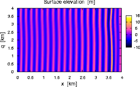
Figure 7: (Color online) [B]. Map of the free surface at $t=172.8$.

Our second numerical experiment (referred to as [B]) is a weakly 3D analog of the 2D numerical experiments performed by Zakharov and co-workers ZDV2002 ; DZ2005Pisma , when a slightly modulated periodic Stokes wave evolves to produce a giant wave. However, with two horizontal dimensions we could not achieve the same very high resolution as Zakharov with co-workers did for the case of a single horizontal dimension ($16384\times 256$ in our experiment [B] versus $2\cdot 10^{6}\times 1$ in Ref. DZ2005Pisma ). Our computations were terminated well before the moment when a giant wave reached its maximum height and began break, since the number of the employed Fourier modes became inadequate. The accuracy could be better with larger $N$ and $L$, and with a smaller $\tau$, but it required much more memory and computational time. In general, to resolve in conformal variables a sharp wave crest with a minimal radius of curvature $\rho$ and with the asymptotic angle $2\pi/3$ (as in the limiting Stokes wave), the required number $K_{eff}$ should adaptively vary as $\rho^{-3/2}\lambda^{1/2}$. The power $-3/2$ results in strong difficulties when $\rho$ is small. Another important point is that Zakharov and co-workers were able to re-formulate the purely 2D equations in terms of the “optimal” complex variables $R=1/Z_{u}$ and $U=i\Psi_{u}/Z_{u}$, thus obtaining very elegant and compact cubic evolution equations (the Dyachenko equations D2001 ). In our 3D case, a similar simplification seems to be impossible, and we dealt directly with the original conformal variables $Z$ and $\Psi$. Nevertheless, our results are sufficiently accurate to reproduce the fact of a giant wave formation.

As the initial state for the experiment [B], we took a weakly modulated periodic wave with the main wave number $k=19$ ($\lambda\approx 210$ m) and with a few first harmonics on $2k$, $3k$, etc., similar to a Stokes wave (not shown). After some period of evolution, the Benjamin-Feir instability developed and resulted in formation of a big wave, with the amplitude 13 m at $t=172.8$ versus the initial maximum amplitude 5 m (see Figs. 5-7 and compare with Ref. DZ2005Pisma ). The peak-to-trough height $h_{*}$ of this computed rogue wave was approximately 20 m at $t=172.8$ (the steepness parameter $h_{*}/\lambda\approx 0.1$), and it was still growing at that moment (so, at $t=173.0$ we observed the amplitude 14 m, but the accuracy was already not sufficient). It is interesting that this numerical solution has a well defined envelope until a very final stage of evolution. Thus, our equations may serve to test the simplified wave-packet models like the extended NLS equations Dysthe1979 ; TKDV2000 ; OOS2000 .

IV Summary and discussion

We have developed an efficient numerical method for modeling the rogue wave phenomenon. The underlying theory for the method is the weakly 3D formulation of the free surface dynamics reported earlier R2005PRE with slight modifications. In particular, the Hamiltonian has been regularized in a way to give the exact linear 2D dispersion relation in the entire Fourier space, and a filter removing shortest waves has been added in the numerical implementation. With these techniques, weakly three-dimensional effects could be included in simulations of rogue wave formation as illustrated in the two examples given. In particular, the genuinely non-linear 2D instability reported by Zakharov et al. ZDV2002 ; DZ2005Pisma could be verified in the weakly 3D regime despite the relatively low resolution (compared to 2D) of $16384\times 256$ points used here.

The results indicate that the assumption of weak variation in the third direction holds even in the late stage of rogue wave formation, which demonstrates the consistency of the expansion in $\epsilon=(l_{x}/l_{q})^{2}$ and thereby the applicability of the present theory.

Planned further steps in the continuation of this work are a more efficient computational implementation through parallelization of the code and the inclusion of additional effects like a bottom profile, which is already covered by the formalism reported earlier R2005PRE .

References

- (1) C. Kharif and E. Pelinovsky, Eur. J. Mech. B/Fluids 22, 603 (2003).
- (2) V. E. Zakharov, A. I. Dyachenko, and O. A. Vasilyev, Eur. J. Mech. B/Fluids 21, 283 (2002).
- (3) A. I. Dyachenko and V. E. Zakharov, Pis’ma v ZhETF 81, 318 (2005) [JETP Letters 81, 255 (2005)].
- (4) T.B. Benjamin and J.E. Feir, J. Fluid Mech. 27, 417 (1967).
- (5) V.E. Zakharov, Sov. Phys. JETP 24, 455 (1967).
- (6) J. W. McLean, Y. C. Ma, D. U. Martin, P. G. Saffman, and H. C. Yuen, Phys. Rev. Lett. 46, 817 (1981).
- (7) V.I. Shrira, S.I. Badulin, and C. Kharif, J. Fluid Mech. 318, 375 (1996).
- (8) F. Collard and G. Caulliez, Phys. Fluids 11, 3195 (1999).
- (9) F. Dias and C. Kharif, Annu. Rev. Fluid Mech. 31, 301 (1999).
- (10) A. I. Dyachenko, E. A. Kuznetsov, M. D. Spector, and V. E. Zakharov, Phys. Lett. A 221, 73 (1996).
- (11) A. I. Dyachenko, V. E. Zakharov, and E. A. Kuznetsov, Fiz. Plazmy 22, 916 (1996) [Plasma Phys. Rep. 22, 829 (1996)].
- (12) V. E. Zakharov and A. I. Dyachenko, Physica D 98, 652 (1996).
- (13) A. I. Dyachenko, Y. V. L’vov, and V. E. Zakharov, Physica D 87, 233 (1995).
- (14) Y. V. Lvov, Phys. Lett. A 230, 38 (1997).
- (15) A. I. Dyachenko, Doklady Akademii Nauk 376, 27 (2001) [Doklady Mathematics 63, 115 (2001)].
- (16) W. Choi and R. Camassa, J. Engrg. Mech. ASCE 125, 756 (1999).
- (17) http://www.fftw.org/
- (18) V. P. Ruban, Phys. Rev. E 70, 066302 (2004).
- (19) V. P. Ruban, Phys. Lett. A 340, 194 (2005).
- (20) W.T. Tsai and D.K.P. Yue, Annu. Rev. Fluid Mech. 28, 249 (1996).
- (21) F. Dias and T. J. Bridges, “The numerical computation of freely propagating time-dependent irrotational water waves”, to be published.
- (22) M.S. Longuet-Higgins and E.D. Cokelet, Proc. Roy. Soc. Lon. A 350, 1 (1976).
- (23) D. Clamond and J. Grue, J. Fluid Mech. 447, 337 (2001).
- (24) D. Fructus, D. Clamond, J. Grue, and Ø. Kristiansen, J. Comput. Phys. 205, 665 (2005).
-
(25)
J.T. Kirby,
in Gravity Waves in Water of Finite Depth, edited by J. N. Hunt,
Advances in Fluid Mechanics, Vol 10
(Computational Mechanics Publications, The Netherlands, 1997), pp. 55-125;
J.T. Kirby, in Advances in Coastal Modeling, edited by V. C. Lakhan (Elsevier, New York, 2003), pp. 1-41;
http://chinacat.coastal.udel.edu/~kirby/kirby_pubs.html - (26) H. B. Bingham and Y. Agnon, Eur. J. Mech. B/Fluids 24, 255 (2005).
- (27) Y. Matsuno, Phys. Rev. E 47, 4593 (1993).
- (28) W. Choi, J. Fluid Mech. 295, 381 (1995).
- (29) M. Onorato, A.R. Osborne, M. Serio, D. Resio, A. Pushkarev, V.E. Zakharov, and C. Brandini, Phys. Rev. Lett. 89, 144501 (2002).
- (30) A.I. Dyachenko, A.O. Korotkevich, and V.E. Zakharov, Phys. Rev. Lett. 92, 134501 (2004).
- (31) K.B. Dysthe, Proc. Roy. Soc. Lon. A 369, 105 (1979).
- (32) K. Trulsen, I. Kliakhadler, K.B. Dysthe, and M.G. Velarde, Phys. Fluids 12, 2432 (2000).
- (33) A.R. Osborne, M. Onorato, and M. Serio, Phys. Lett. A 275, 386 (2000).
- (34) P.A.E.M. Janssen, J. Phys. Oceanogr. 33, 863 (2003).
- (35) V. P. Ruban, Phys. Rev. E 71, 055303(R) (2005).
- (36) V. E. Zakharov, Eur. J. Mech. B/Fluids 18, 327 (1999).
- (37) V. P. Ruban and J. J. Rasmussen, Phys. Rev. E 68, 056301 (2003).
- (38) P. M. Lushnikov and V. E. Zakharov, Physica D 203, 9 (2005).