Laser–dressed vacuum polarization in a Coulomb field

Abstract

We investigate quantum electrodynamic effects under the influence of an external, time-dependent electromagnetic field, which mediates dynamic modifications of the radiative corrections. Specifically, we consider the quantum electrodynamic vacuum-polarization tensor under the influence of two external background fields: a strong laser field and a nuclear Coulomb field. We calculate the charge and current densities induced by a nuclear Coulomb field in the presence of a laser field. We find the corresponding induced scalar and vector potentials. The induced potential, in first-order perturbation theory, leads to a correction to atomic energy levels. The external laser field breaks the rotational symmetry of the system. Consequently, the induced charge density is not spherically symmetric, and the energy correction therefore leads to a “polarized Lamb shift.” In particular, the laser generates an additional potential with a quadrupole moment. The corresponding laser-dressed vacuum-polarization potential behaves like $1/r^{3}$ at large distances, unlike the Uehling potential that vanishes exponentially for large $r$. The energy corrections are of the same order-of-magnitude for hydrogenic levels, irrespective of the angular momentum quantum number. The induced current leads to a transition dipole moment which oscillates at the second harmonic of the laser frequency and is mediated by second-order harmonic generation in the vacuum-polarization loop. In the far field, at distances $r\gg 1/\omega$ from the nucleus ($\omega$ is the laser frequency), the laser induces mutually perpendicular electric and magnetic fields, which give rise to an energy flux that corresponds to photon fusion leading to the generation of real photons, again at the second harmonic of the laser. Our investigation might be useful for other situations where quantum field theoretic phenomena are subjected to external fields of a rather involved structure.

I INTRODUCTION

This article is concerned with the calculation of the vacuum-polarization tensor in the presence of two nontrivial background fields: a nuclear Coulomb field and a (possibly strong) laser field. Particular emphasis is laid on the induced charge density and potential, as well as the induced current and the vector potential, and the resulting induced electromagnetic fields. As an application, we consider the energy shifts of atomic states in hydrogenlike systems, and induced transition probabilities, under the influence of the laser-dressed vacuum polarization. However, we would like to emphasize that the two latter aspects constitute merely example applications of the more general expressions derived in this article.

Before we indulge into this endeavour, let us briefly recall a few very well known facts about vacuum polarization. It is well known that the Coulomb law becomes invalid at distances comparable to the electron Compton wavelength $\lambdabar_{\rm e}=3.8\times 10^{-11}\,{\rm cm}$. This phenomenon is due to the excitation of virtual electron-positron pairs from the vacuum, which polarize the vacuum in a way approximately equivalent to a dielectric medium. Indeed, at large distance, we see only a “screened” charge, which is less than the “bare” charge visible to an observer who approaches the particle in question, in our case mostly an atomic nucleus, to a very close distance. The total charge density induced in the vacuum has to be zero, and this also defines the renormalization condition for the charge which can be defined via the low-energy limit of the Thomson scattering cross section (see ItZu1980 , Chap. 7), as it affects two distant charge particles. However, as we enter the cloud of the electron-positron pairs that surround the charged nucleus, the effective charge becomes larger, because one has to add to the “renormalized”, physical charge of the nucleus (seen at large distance), a contribution due to the electron-positron pairs that surround the nucleus at short distance.

So, the virtual excitations of the electron-positron (or muon-antimuon) pairs naturally generate a “fifth-force” like Yukawa potential contribution to the Coulomb law, which is however exponentially suppressed at distances larger than the Compton wavelength, and by a quantum electrodynamic (QED) perturbation theory parameter $\alpha$.

What happens to the vacuum-polarization effects in a laser field? Evidently, the laser field, which is composed of many photons, will modify the electron-positron loop as the laser photons interact with the virtual quanta during their short lifetime that is only of the order of $\lambdabar_{\rm e}/c=1.3\times 10^{-21}\,{\rm s}$. We find that in a remarkably strong laser field, the modification of the vacuum-polarization contribution to the Coulomb law can be significant. In particular, the laser induces a rotational symmetry breaking in the correction to the Coulomb law, which leads to a polarized Lamb shift whereby states with different magnetic quantum numbers receive different energy shifts. The induced charge density, in a laser field, has a monopole and a quadrupole component. The quadrupole part of the potential is not exponentially suppressed at large distances, but tails off like a “normal” quadrupole potential, i.e. as $1/r^{3}$.

In part, our investigation follows ideas outlined previously in the context of the analysis of the vacuum-polarization tensor in a laser field BaMiSt1975 ; BeMi1975 . Here, our focus is on applications including a (possibly strong) binding Coulomb field in addition to the laser field. Another fundamental QED process, the self-energy under the influence of an external laser field, for a free particle, has previously been studied in BaKaMiSt1975 ; BeMi1976 , and for a strongly driven transition between bound states, in JeEvHaKe2003 ; JeKe2004aop ; EvJeKe2004 ; JeEvKe2005 . A more general context of our study might be defined as “quantum field theory under the influence of external fields.”

From a naive point of view, one might expect that in a strong laser field, the charge density induced by the vacuum polarization loses the rotational symmetry, and that an alignment along the laser propagation and polarization axes occurs. However, the exact functional form of the induced laser-dressed contribution to the charge density [see Eq. (26) below] is not accessible by symmetry arguments. It is therefore indispensable to use a fully laser-dressed formalism, where the quantum electrodynamic effects are incorporated into the propagators right from the start of the calculation. As will be discussed below, the result of a fully laser-dressed calculation confirms the intuitive picture, according to which rotational invariance is broken in both linear as well as circularly polarized laser fields, and a few unexpected asymptotic structures are found for the laser-induced fields.

This article is organized as follows: in Sec. II, we analyze the additional charge density induced by the external laser field (this potential is an addition to the “normal” Uehling potential). The way from the charge density to the induced potential is detailed in Sec. II.1. The asymptotics of the induced potential, in various regions from the atomic nucleus, are derived in Sec. II.2. As an application, the energy shift of hydrogenic bound states is considered in Sec. II.3.

II INDUCED CHARGE DENSITY AND POTENTIAL

II.1 From the charge density to the potential

The amplitude $\cal T$ of photon scattering in the laser field has the form

$${\cal T}=\varepsilon_{2}^{\mu*}\,T_{\mu\,\nu}(k_{2},k_{1})\,\varepsilon_{1}^{\nu}\,.$$ (1)

Here, the four-vectors $k_{1}$ and $k_{2}$ characterize the incoming and outgoing photon momenta, as they flow into and out of the laser-dressed loop. The polarization vectors of the photons are $\varepsilon_{1}^{\mu}$ and $\varepsilon_{2}^{\mu}$. The quantity $T_{\mu\,\nu}(k_{2},k_{1})$ is canonically identified as the vacuum-polarization tensor. The calculation of the tensor $T_{\mu\,\nu}(k_{2},k_{1})$ is a rather involved calculation, but complete results, valid for arbitrary laser-field configurations, were found with the use of operator techniques in Ref. BaMiSt1975 . Independently, by means of another method, the vacuum-polarization tensor was obtained in Ref. BeMi1975 . Both results are in agreement with each other. Of course, the scattering, which is beyond Maxwell’s classical electrodynamics, appears due to the polarization of the electron-positron vacuum in the presence of a laser field.

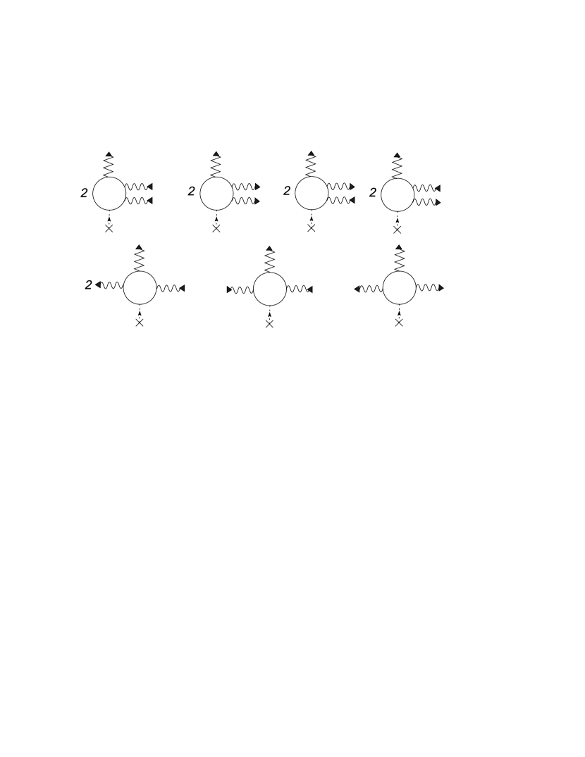
\begin{picture}(0.0,0.0)(0.0,0.0)\end{picture}

Figure 1: Diagrams corresponding to the amplitude (II.1), including their multiplicities. The solid lines are the electron propagators, the dashed line with the cross denotes the Coulomb field, the wavy lines correspond to the laser photons, and the zigzag line is the induced field.

In this article, we use rationalized Gaussian units with $\hbar=c=1$, and $\epsilon_{0}=(4\pi)^{-1}$, which implies $e^{2}=\alpha$ where $e$ is the electron charge and $\alpha$ is the fine-structure constant. We represent the vector potential of the laser field in the form

$$A_{\mu}(\phi)=e_{1\mu}\psi_{1}(\phi)+e_{2\mu}\psi_{2}(\phi)\,.$$ (2)

Here, $\phi=\varkappa x=\varkappa^{0}t-{\vec{\varkappa}}{\vec{r}}$ is the phase of the laser field at the space-time point $(\vec{r},t)$, and $\omega=\varkappa^{0}=|\vec{\varkappa}|$ is the laser frequency. We use the spacetime metric in the Bjorken–Drell convention $g_{\mu\nu}={\rm diag}(1,-1,-1,-1)$. The vector $\vec{\varkappa}$ points into the laser propagation direction, and $\psi_{1,2}(\phi)$ are functions which characterize the shape of the laser pulse. We denote the (orthogonal) unit vectors giving the polarization directions by ${\vec{e}}_{1}$ and ${\vec{e}}_{2}$, respectively (${\vec{e}}^{2}_{1}={\vec{e}}^{2}_{1}=1)$. The corresponding four-vectors $e_{1}=(0,\vec{e}_{1})$ and $e_{2}=(0,\vec{e}_{2})$ satisfy

$$\varkappa^{2}=\varkappa\cdot e_{1}=\varkappa\cdot e_{2}=e_{1}\cdot e_{2}=0\,,\quad e_{1}^{2}=e_{2}^{2}=-1\,.$$ (3)

All vector scalar products (involving three or four-vectors) are denoted by $\cdot$ in this article. We also use the conventions

$${\vec{\nu}}=\frac{\vec{\varkappa}}{\omega},\qquad{\vec{n}}=\frac{{\vec{r}}}{r}$$ (4)

for the unit vector ${\vec{\nu}}={\vec{e}}_{1}\times{\vec{e}}_{2}$ pointing into the propagation direction, and the unit vector pointing to a coordinate ${\vec{r}}$, respectively.

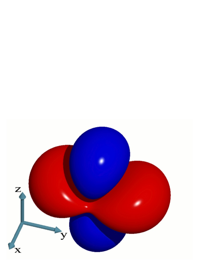
Figure 2: (Color online.) The familiar rotationally symmetric vacuum-polarization charge density around an atomic nucleus is severely distorted in a strong laser field. Here, we plot the additional laser-dressed, time-independent contribution to the renormalized charge density $\delta\rho^{R}_{0}(\vec{r})$, as induced by the laser field. The quantity $\delta\rho^{R}_{0}(\vec{r})$ has to be added to the well-known expressions for the Uehling and the Wichmann–Kroll parts (for a review see e.g. MoPlSo1998 ). The result for $\delta\rho^{R}_{0}(\vec{r})$ is obtained after Fourier transformation of the momentum-space result given in Eq. (II.1) below, into coordinate space. Along the vertical axis, we have the propagation direction of the laser, which we assume to be linearly polarized ($\xi_{1}^{2}\neq 0$, $\xi_{2}^{2}=0$). The polarization direction (laser electric field) is along the $x$-axis. We plot a characteristic surface given by a constant induced charge density, namely the surface defined by the relation $\delta\rho_{0}(\vec{r})=\frac{2\alpha}{3\pi}\,\frac{Ze\,m^{3}}{\pi}\,\left({\cal E}/{\cal E}_{0}\right)^{2}\,K$, where $K$ is a numerical constant given by $K=\pm 1.204$ for the plot shown. Two areas with a positive induced charge density (red, aligned mainly along the $y$ axis, $K=+1.204$) and a negative one are distinguished (the latter is in blue color and located along the propagation axis, $K=-1.204$). As emphasized in the text, the total induced charge is zero.

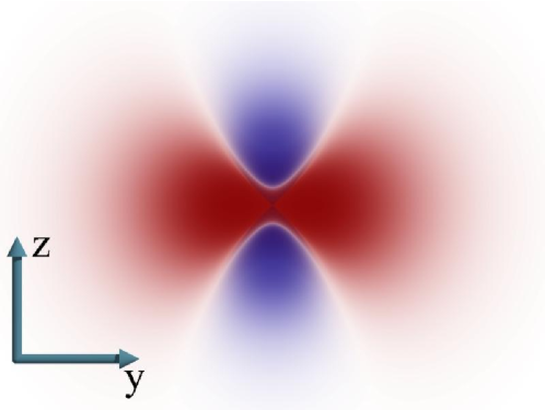
(a)

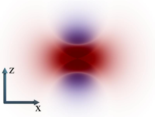
(b)

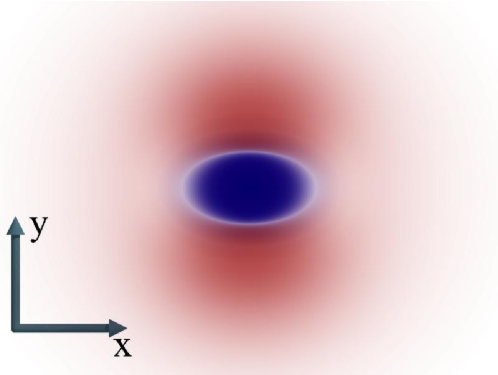
(c)

Figure 3: (Color online.) Projections of the laser-induced part of the vacuum-polarization charge density looked upon from the $x$, $y$ and $z$ axis, in Figs. (a), (b) and (c), respectively. The conventions are the same as in Fig. 2: the $z$-axis is the laser propagation direction, and the $x$-axis is the polarization axis (laser electric field). The picture provides a ray-traced impression of the charge density, represented as an absorptive medium. Red color is used for positive induced charge (areas located along the $x$ and $y$ axes), blue color is used for negative charge (areas located along the $z$ axis). The plots are as seen by an observer looking at the atomic nucleus from the specified directions. This is in contrast to Fig. 2, where the isosurface corresponding to a given, constant charge density is plotted. In the above graphical representations, the fall-off of the induced charge density for large radial arguments can be distinguished clearly.

In Refs. BaMiSt1975 ; BeMi1975 , the photon scattering amplitude was found for arbitrary functions $\psi_{1,2}$. In the current paper, we restrict ourselves to the case of monochromatic plane wave with the frequency $\omega$, although with allowance for arbitrary (linear, elliptic) polarizations. In this case, the functions $\psi_{1}(\phi)$ and $\psi_{2}(\phi)$ take the form

$$\psi_{1}(\phi)=a_{1}\cos\phi\,,\quad\psi_{2}(\phi)=a_{2}\sin\phi\,,\quad\varkappa^{0}=\omega\,.$$ (5)

The scattering amplitude depends on the parameters

$$\xi^{2}_{1,2}=\frac{e^{2}a^{2}_{1,2}}{m^{2}}\,,\quad\lambda=\frac{\varkappa\cdot k_{1}}{2m^{2}}=\frac{\varkappa\cdot k_{2}}{2m^{2}}\,,$$ (6)

where $m$ is the electron mass. The mean square laser field strength ${\cal E}^{2}$, averaged over a laser period, is expressed via the parameters $\xi^{2}_{1,2}$ by the relation

$$\left(\frac{e}{m\,\omega}\right)^{2}\,{\cal E}^{2}=\frac{1}{2}(\xi_{1}^{2}+\xi_{2}^{2})\,,\quad\,.$$ (7)

Thus, we may say that the parameters $\xi_{1,2}$ measure the laser field strength. The parameter $\lambda$, by contrast, measures the momentum scales relevant to the vacuum-polarization loop (incoming momenta and the four-momentum of the laser wave) against the electron mass scale.

The following identity is sometimes useful:

$$\frac{1}{2}\,\frac{\omega^{2}}{m^{2}}(\xi^{2}_{1}+\xi^{2}_{1})=\left(\frac{\cal E}{{\cal E}_{0}}\right)^{2}\,.$$ (8)

Here, ${\cal E}_{0}$ is the Schwinger critical electric field strength ${\cal E}_{0}={m^{2}}/{e}=4.4\times 10^{15}\,\mbox{V\,cm}^{-1}$.

As is well known, the presence of an external field leads to the existence of an induced current $J^{\mu}$ due to the vacuum polarization. If the external field is a pure Coulomb field, then for the induced current we have ${\vec{J}}=0$, and $\rho=J^{0}$ is well known in this case (see, e.g., BeLiPi1982 ). Here, we consider the situation where the external field is a Coulomb field, but there is, in addition, the laser field, which dresses the vacuum-polarization loop.

Our incoming photon is the Coulomb quantum with $k_{1}=q=(0,{\vec{q}})$ and $\varepsilon_{1}^{\mu}=\delta^{\mu}_{0}$. Then, $J^{\mu}=T^{\mu\,0}(k_{2},k_{1})$. We calculate $J^{\mu}$ in the leading approximation in the parameter $Z\alpha$, where $Z$ is the nuclear charge number. Due to momentum and $C$–parity conservation (Furry theorem), we have $k_{2}=k_{1}+2l\varkappa$, where $l=0,\pm 1,\pm 2...$, and this fact affords an explanation for the two alternative definitions of $\lambda$ in Eq. (6). A noticeable contribution to the induced charge density arises at distances $r\simeq\lambdabar_{\rm e}=1/m$ , which reciprocally corresponds to the momentum of a Coulomb quantum $|{\vec{q}}|\simeq m$.

For all current high-intensity lasers, the laser photon energy is small as compared to the electron rest mass energy ($\omega\ll m$), and therefore

$$|\lambda|\sim\frac{|{\vec{q}}|\,\omega}{m^{2}}\leq\frac{\omega}{m}\ll 1\,.$$ (9)

Our calculations as reported in the current article depend on the approximation $\lambda\ll 1$ [see also Eqs. (2.5), (2.31) and (2.32) of Ref. BaMiSt1975 ]. All results reported below are given on the first nonvanishing order in the expansion in powers of $\omega/m$. A further condition imposed on our calculations concerns the laser intensity parameters $\xi_{1,2}$,

$$0<\xi^{2}_{1,2}\ll 1/\lambda^{2}\,,$$ (10a)

which according to Eq. (8) means that

$$\frac{{\cal E}}{{\cal E}_{0}}\ll 1\,.$$ (10b)

The asymptotics of $T^{0\,0}(k_{2},k_{1})=T^{0\,0}(k_{2},q)$ under this approximation are found to consist of terms with absorption and emission of one laser photon each, and of terms with absorption of two and emission of two laser photons (see Fig. 1),

$$T^{0\,0}(k_{2},q)=(2\pi)^{4}\,\left[\delta(q-k_{2})\,B^{(0)}({\vec{q}})\right.$$

$$\left.+\delta(q-k_{2}-2\varkappa)\,B^{(-)}({\vec{q}})+\delta(q-k_{2}+2\varkappa)\,B^{(+)}({\vec{q}})\right]\,.$$ (11)

in the matrix element. Here, the functions $B^{(0)}({\vec{q}})$ and $B^{(\pm)}({\vec{q}})$ are given by

$$B^{(0)}({\vec{q}}) = \frac{\alpha\,\omega^{2}}{24\pi\,m^{2}}\,\int\limits_{0}^{1}dv\,(1-v^{2})^{2}\,D^{2}\biggl{\{}-\frac{3}{4}(\xi_{1}^{2}-\xi_{2}^{2})(q_{1}^{2}-q_{2}^{2})\,$$ (12a)

$$+\frac{(\xi_{1}^{2}+\xi_{2}^{2})}{(1-v^{2})}\,\left[(q_{1}^{2}+q_{2}^{2})(1+v^{2}+D)+\frac{({\vec{q}}^{\,2})^{2}}{4m^{2}}(1-v^{2})^{2}D\right]\biggr{\}}\,,$$

$$B^{(\pm)}({\vec{q}}) = \frac{\alpha\,\omega^{2}}{48\pi\,m^{2}}\,\int\limits_{0}^{1}dv\,(1-v^{2})^{2}\,D^{2}\,\biggl{\{}\pm 3\,i\,\xi_{1}\xi_{2}\,q_{1}\,q_{2}+\frac{3}{4}(\xi_{1}^{2}+\xi_{2}^{2})(q_{1}^{2}-q_{2}^{2})$$ (12b)

$$-\frac{(\xi_{1}^{2}-\xi_{2}^{2})}{(1-v^{2})}\left[(q_{1}^{2}+q_{2}^{2})(1+v^{2}+D)+\frac{({\vec{q}}^{\,2})^{2}}{4m^{2}}(1-v^{2})^{2}\,D\right]\biggr{\}}\,,$$

where

$$q_{1}={\vec{q}}\cdot{\vec{e}}_{1},\quad q_{2}={\vec{q}}\cdot{\vec{e}}_{2},$$

$$D\equiv D(\vec{q}^{\,2})=\left[1+\frac{{\vec{q}}^{\,2}(1-v^{2})}{4m^{2}}\right]^{-1}\,.$$ (13)

In the derivation of Eq. (12), we have neglected higher-order terms in the expansion in powers of $\omega/m$. The Fourier transform of the correction to the induced charge density due to the laser field, $\delta\rho(\vec{q},t)$, is essentially given by the Fourier transform of $T^{0\,0}(k_{2},q)$. It is a sum of time-dependent and time-independent parts:

$$\delta\rho({\vec{q}},t) = \delta\rho_{0}({\vec{q}})+\delta\rho_{1}({\vec{q}},t)\,,$$ (14)

where

$$\frac{\delta\rho_{0}({\vec{q}})}{Ze}= \frac{1}{{\vec{q}}^{\,2}}B^{(0)}({\vec{q}})\,,$$ (15)

$$\frac{\delta\rho_{1}({\vec{q}},t)}{Ze}= \frac{e^{2i\omega t}}{({\vec{q}}+2{\vec{\varkappa}})^{2}}B^{(-)}({\vec{q}})+\frac{e^{-2i\omega t}}{({\vec{q}}-2{\vec{\varkappa}})^{2}}\,B^{(+)}({\vec{q}}).$$

We now turn to a more specific evaluation of the charge density, in various regions of practical interest. First, we investigate (in coordinate space) the distance $r\sim a_{0}=1/(Z\alpha m)$, which typically gives rise to the main corrections to the energy in bound systems ($a_{0}$ is the Bohr radius). For a laser whose frequency is of the order of atomic transitions, we have $\omega\sim(Z\alpha)^{2}m\ll 1/a_{0}$, so that the “interesting” distance fulfill $r\ll 1/\omega$, and the corresponding momenta are in the range $q\sim 1/r\gg\omega=|\vec{\varkappa}|$. We can therefore replace

$$({\vec{q}}\pm 2{\vec{\varkappa}})^{2}\to{\vec{q}}^{\,2}$$ (16)

in Eq. (15). Note that this replacement, in particular, does not affect the validity of the expressions for radial arguments of the order of the Compton wavelength. Employing the approximation (16), we obtain from Eqs. (12), (14) and (15)

$$\delta\rho_{0}({\vec{q}})=\frac{\alpha(Ze)\omega^{2}}{24\pi\,m^{2}{\vec{q}}^{\,2}}\int\limits_{0}^{1}dv\,(1-v^{2})^{2}\,D^{2}$$

$$\times\biggl{\{}-\frac{3}{4}(q_{1}^{2}-q_{2}^{2})(\xi_{1}^{2}-\xi_{2}^{2})\,+\left[\frac{(q_{1}^{2}+q_{2}^{2})}{(1-v^{2})}(1+v^{2}+D)\right.$$

$$\quad\left.+\frac{({\vec{q}}^{\,2})^{2}}{4m^{2}}(1-v^{2})\,D\right](\xi_{1}^{2}+\xi_{2}^{2})\biggr{\}}\,,$$ (17a)

and

$$\delta\rho_{1}({\vec{q}},t)=\frac{\alpha(Ze)\omega^{2}}{24\pi\,m^{2}{\vec{q}}^{\,2}}\int\limits_{0}^{1}dv\,(1-v^{2})^{2}\,D^{2}$$ (17b)

$$\times\biggl{\{}\frac{3}{4}(q_{1}^{2}-q_{2}^{2})(\xi_{1}^{2}\,+\xi_{2}^{2})\cos(2\omega t)$$

$$\quad-\left[\frac{(q_{1}^{2}+q_{2}^{2})}{(1-v^{2})}(1+v^{2}+D)+\frac{({\vec{q}}^{\,2})^{2}}{4m^{2}}(1-v^{2})\,D\right]$$

$$\qquad\times(\xi_{1}^{2}-\xi_{2}^{2})\cos(2\omega t)+3\xi_{1}\,\xi_{2}\,q_{1}\,q_{2}\,\sin(2\omega t)\biggr{\}}\,.$$

Although the expression for the vacuum polarization tensor in Eqs. (2.5), (2.31) and (2.32) of Ref. BaMiSt1975 is in principle already renormalized, it is still necessary to carry out an additional finite subtraction, namely, to subtract the asymptotics of the induced charge at $|{\vec{q}}|\rightarrow 0$. This is akin to the additional subtractions that have to be carried out in the calculation of the Wichmann–Kroll correction. The renormalization condition in the on-mass-shell scheme, for the Coulomb field is that two distant observers should observe exactly the Thomson scattering cross section, which implies that the total induced charge has to be equal to zero (an eludicating discussion surrounds Eq. (7.18) of Ref. ItZu1980 ). In addition, our subtraction provides a finite quadrupole moment, corresponding to the induced charge distribution. Because $\delta\rho_{1}({\vec{q}},t)\rightarrow 0$ at $|{\vec{q}}|\rightarrow 0$ [see Eq.(15)], it is only the time-independent part $\delta\rho_{0}({\vec{q}})$ which receives an additional, finite renormalization.

The subtraction leads to the renormalized time-independent component of the charge density $\delta\rho_{0}^{R}({\vec{q}})$,

$$\delta\rho_{0}^{R}({\vec{q}})=\delta\rho_{0}({\vec{q}})-\frac{\alpha(Ze)\omega^{2}}{60\pi\,m^{2}{\vec{q}}^{\,2}}$$

$$\times\left[\frac{11}{3}\,(\xi_{1}^{2}+\xi_{2}^{2})(q_{1}^{2}+q_{2}^{2})-(\xi_{1}^{2}-\xi_{2}^{2})(q_{1}^{2}-q_{2}^{2})\right]\,.$$ (18)

The renormalized charge density $\delta\rho_{0}^{R}({\vec{r}})$, excluding the Dirac delta contribution, is represented graphically in Figs. 2 and 3. The full renormalized $\delta\rho^{R}({\vec{q}},t)$ (including the time-dependent term) is

$$\delta\rho^{R}({\vec{q}},t)=\delta\rho_{0}^{R}({\vec{q}})+\delta\rho_{1}({\vec{q}},t)\,.$$ (19)

The potential $\Phi({\vec{r}},t)$ in the Lorentz gauge satisfies the equation

$$\frac{\partial^{2}}{\partial t^{2}}\,\Phi({\vec{r}},t)-\vec{\nabla}^{2}\Phi({\vec{r}},t)=4\pi\,\delta\rho^{R}({\vec{r}},t)\,.$$ (20)

Therefore, the Fourier transform of the potential, which corresponds to the density $\delta\rho^{R}({\vec{q}},t)$, is

$$\Phi({\vec{q}},t) = \frac{4\pi}{{\vec{q}^{2}}}\,\delta\rho_{0}^{R}({\vec{q}})+\frac{4\pi}{{\vec{q}}^{\,2}-4\omega^{2}}\,\delta\rho_{1}({\vec{q}},t)$$ (21)

$$= \frac{4\pi}{{\vec{q}^{2}}}\,\delta\rho_{0}^{R}({\vec{q}})+4\pi(Ze)\left[\frac{e^{2i\omega t}B^{(-)}({\vec{q}})}{({\vec{q}}^{\,2}-4\omega^{2}+i0)({\vec{q}}+2{\vec{\varkappa}})^{2}}+\frac{e^{-2i\omega t}B^{(+)}({\vec{q}})}{({\vec{q}}^{\,2}-4\omega^{2}-i0)({\vec{q}}-2{\vec{\varkappa}})^{2}}\right]\,.$$

Here the regularization of the denominators, ($\pm i0$), corresponds to the boundary condition of radiation (see below). It is convenient to present the potential in coordinate space as a sum of time-dependent and time-independent parts:

$$\Phi({\vec{r}},t)=\Phi_{0}({\vec{r}})+\Phi_{1}({\vec{r}},t)\,.$$ (22)

By Fourier transform of Eq. (21), we thus obtain at a distance $r\ll 1/\omega$ from the nucleus,

$$\Phi_{0}({\vec{r}}) = \frac{\alpha(Ze)\omega^{2}}{48\pi\,m}\biggl{\{}\left[F_{1}(mr)+F_{2}(mr)\left(1-3({\vec{\nu}}\cdot{\vec{n}})^{2}\right)\right](\xi_{1}^{2}+\xi_{2}^{2})$$ (23a)

$$-F_{3}(mr)\left[({\vec{n}}\cdot{\vec{e}}_{1})^{2}-({\vec{n}}\cdot{\vec{e}}_{2})^{2}\right](\xi_{1}^{2}-\xi_{2}^{2})\biggr{\}}\,,$$

$$\Phi_{1}({\vec{r}},t) = -\frac{\alpha(Ze)\omega^{2}}{48\pi\,m}\biggl{\{}\left[\left(F_{1}(mr)+\frac{88}{45mr}\right)+\left(F_{2}(mr)-\frac{22}{45mr}\right)\left(1-3({\vec{\nu}}{\vec{n}})^{2}\right)\right](\xi_{1}^{2}-\xi_{2}^{2})\cos(2\omega t)$$ (23b)

$$-\left(F_{3}(mr)-\frac{2}{5mr}\right)\left[(\xi_{1}^{2}+\xi_{2}^{2})\cos(2\omega t)\left[({\vec{n}}\cdot{\vec{e}}_{1})^{2}-({\vec{n}}\cdot{\vec{e}}_{2})^{2}\right]+4\xi_{1}\xi_{2}\sin(2\omega t)({\vec{n}}\cdot{\vec{e}}_{1})({\vec{n}}\cdot{\vec{e}}_{2})\right]\biggr{\}},$$

where we note the conventions in Eqs. (3) and (4). In this formula,

$$F_{1}(mr) = \int\limits_{0}^{1}dv\,(1-v^{2})^{1/2}\left\{\frac{1}{2}(1-v^{2})(1+2y)-\frac{4}{3y}\,\left[(1+v^{2})(1+y)+1+\frac{5}{4}y+\frac{1}{2}y^{2}\right]\right\}e^{-2y}\,,$$ (24a)

$$F_{2}(mr) = \int\limits_{0}^{1}dv\,(1-v^{2})^{1/2}\,\biggl{\{}\frac{1}{3y}\left[(1+v^{2})(1+y)+1+\frac{5}{4}y+\frac{1}{2}y^{2}\right]e^{-2y}$$ (24b)

$$+\frac{1+v^{2}}{y^{3}}\left[1-(1+y)(1+y+y^{2})e^{-2y}\right]+\frac{3}{2y^{3}}\left[1-(1+2y+2y^{2}+\frac{7}{6}y^{3}+\frac{1}{3}y^{4})e^{-2y}\right]\biggr{\}}\,,$$

$$F_{3}(mr) = \frac{9}{4}\,\int\limits_{0}^{1}dv\,\frac{(1-v^{2})^{3/2}}{y^{3}}\left[1-(1+y)(1+y+\frac{2}{3}y^{2})\,e^{-2y}\right]\,,$$

$$y \equiv y(r,v)=\frac{mr}{\sqrt{1-v^{2}}}\,.$$ (24c)

In principle, the expressions (23) gives the complete answer for the induced potential, which is necessary for the calculation of the energy shift. We reemphasize that the only additional approximation employed was $\lambda\ll 1$, which is easily fulfilled for current and planned high-intensity laser facilities. Note that in the particular case of the circular polarized laser field ($\xi_{1}=\pm\xi_{2}=\xi$), the expression for the induced potential becomes essentially simpler.

II.2 Asymptotics of the induced potential

Let us consider the behaviour of the potential (23) at large and small distances. The functions $F_{i}(\rho)$ have the following asymptotics at $\rho=mr\gg 1$:

$$F_{1}(\rho)\simeq\frac{\sqrt{\pi\rho}}{6}e^{-2\rho}\,,\;F_{2}(\rho)\simeq\frac{148}{105\rho^{3}}\,,\;F_{3}(\rho)\simeq\frac{36}{35\rho^{3}}.$$ (25)

We can thus safely neglect the exponentially decaying $F_{1}(\rho)$-term against the polynomial behaviour of $F_{2}$ and $F_{3}$ for $r\gg 1/m$. We recall that the representation in Eqs. (23) and (24) is valid under the (additional) condition $r\ll 1/\omega$. Thus, we write the asymptotics of the potential at $1/\omega\gg r\gg 1/m$ in the form

$$\Phi({\vec{r}},t) \simeq \frac{n^{i}\,n^{j}Q^{ij}}{2r^{3}}+\frac{1}{r}f({\vec{n}},t)\,,$$ (26)

$$f({\vec{n}},t) = -\frac{\alpha(Ze)\omega^{2}}{360\pi\,m^{2}}\biggl{\{}11\left[1+({\vec{\nu}}\cdot{\vec{n}})^{2}\right](\xi_{1}^{2}-\xi_{2}^{2})\cos(2\omega t)$$ (27)

$$+3(\xi_{1}^{2}+\xi_{2}^{2})\cos(2\omega t)\left[({\vec{n}}\cdot{\vec{e}}_{1})^{2}-({\vec{n}}\cdot{\vec{e}}_{2})^{2}\right]$$

$$+12\xi_{1}\xi_{2}\sin(2\omega t)\,({\vec{n}}\cdot{\vec{e}}_{1})\,({\vec{n}}\cdot{\vec{e}}_{2})\biggr{\}}\,.$$

The first term on the right-hand side of Eq. (26), proportional to $1/r^{3}$, can be associated in a natural way with a charge distribution that originates from an oscillatory quadrupole moment,

$$Q^{ij} = \frac{3\alpha(Ze)\omega^{2}}{35\pi\,m^{4}}\biggl{\{}\frac{37}{27}\left(\delta^{ij}-3\nu^{i}\nu^{j}\right)\left[\xi_{1}^{2}\sin^{2}(\omega t)+\xi_{2}^{2}\cos^{2}(\omega t)\right]$$ (28)

$$-(e_{1}^{i}e_{1}^{j}-e_{2}^{i}e_{2}^{j})\left[\xi_{1}^{2}\sin^{2}(\omega t)-\xi_{2}^{2}\cos^{2}(\omega t)\right]-(e_{1}^{i}e_{2}^{j}+e_{2}^{i}e_{1}^{j})\xi_{1}\xi_{2}\sin(2\omega t)\biggr{\}}\,.$$

The second term on the right-hand side of (26), proportional to $1/r$, reflects the existence of radiation in the system, but cannot be used for a valid description of the radiation. The reason is that the derivation of the asymptotics (26) was carried out at distances $1/m\ll r\ll 1/\omega$. This is insufficient for the consideration of radiation, which by definition is only a well-defined process at distances much larger than the wavelength of the emitted light. For the calculation of the radiation, it is necessary to consider distances $r\gg 1/\omega$ (see Sec. III.4) below.

As was already pointed out, for the purpose of calculating the energy shift, it is necessary to know the time-independent part of the potential (for the oscillatory terms, the time-averaging is applied over a full period of the driving laser). The time-averaged part of the quadrupole moment has the form:

$$Q_{0}^{ij}= \frac{3\alpha(Ze)\omega^{2}}{70\pi\,m^{4}}\biggl{\{}\frac{37}{27}\left(\delta^{ij}-3\nu^{i}\nu^{j}\right)(\xi_{1}^{2}+\xi_{2}^{2})$$

$$-(e_{1}^{i}e_{1}^{j}-e_{2}^{i}e_{2}^{j})(\xi_{1}^{2}-\xi_{2}^{2})\biggr{\}}\,.$$ (29)

At small distances from the nucleus, $r\ll 1/m$, we get a complete different asymptotic behaviour for the functions $F_{i}(\rho)$,

$$F_{1}(\rho)\simeq-\frac{88}{45\rho}\,,\quad F_{2}(\rho)\simeq\frac{22}{45\rho}\,,\quad F_{3}(\rho)\simeq\frac{2}{5\rho}\,.$$ (30)

For the potential, this implies

$$\Phi({\vec{r}},t) \simeq -\frac{\alpha(Ze)\omega^{2}}{360\pi\,m^{2}\,r}\biggl{\{}11\left[1+({\vec{\nu}}\cdot{\vec{n}})^{2}\right](\xi_{1}^{2}+\xi_{2}^{2})$$ (31)

$$+3\left[({\vec{n}}\cdot{\vec{e}}_{1})^{2}-({\vec{n}}\cdot{\vec{e}}_{2})^{2}\right](\xi_{1}^{2}-\xi_{2}^{2})\biggr{\}}\,.$$

We see that the leading small-distance asymptotics is independent of time.

II.3 Application: energy shift of hydrogenic levels

Let us consider the correction $\delta E=\left<\,e\Phi_{0}({\vec{r}})\,\right>$ to hydrogenic energy levels, corresponding to the potential $\Phi_{0}({\vec{r}})$, Eq.(23). For $n\,s_{1/2}$-states, only the spherically symmetric part of this potential gives a nonzero contribution. It is proportional to the function $F_{1}(mr)$. Because the function $F_{1}(mr)$ decreases exponentially at $mr\gg 1$, we can replace in the matrix element the wave function $\psi(r)$ by $\psi(0)$, because it has the electron Compton wavelength is much smaller than the characteristic scale $a_{0}=1/(Z\alpha m)\gg 1/m$.

With the considerations, the energy shift for $S$ states can be easily calculated, and we obtain [see Eqs. (8), (23) and (25)]

$$\delta E(nS) = -\frac{8\alpha(Z\alpha)^{4}\omega^{2}}{135\pi\,n^{3}m}(\xi_{1}^{2}+\xi_{2}^{2})$$ (32)

$$= -\frac{16\alpha(Z\alpha)^{4}\,m}{135\pi\,n^{3}}\left(\frac{{\cal E}}{{\cal E}_{0}}\right)^{2}\,.$$

Therefore, due to the factor ${\cal E}/{\cal E}_{0}$, in all realistic cases the correction obtained is small.

Let us consider the corrections to the energy level with the orbital angular momentum $l>0$. In the general case of an elliptically polarized wave ($\xi_{1}\neq\xi_{2}$) , the projection $j_{z}$ of the total angular momentum on the propagation direction of the laser $\vec{\nu}$ is not conserved. This implies a nonvanishing nondiagonal matrix element of the potential $\Phi_{0}({\vec{r}})$ for $\Delta j_{z}=\pm 2$. For $j\geq 3/2$ (where $j$ is the total electron angular momentum), it is necessary to solve a more complicated secular equation in order to find the eigenvalues in the presence of the laser-dressed vacuum polarization. For simplicity, we restrict ourselves to the case of a circular polarized laser field, where the mentioned problem does not appear, and all matrix elements remain diagonal.

For $l\neq 0$, the main contribution to the integral for the matrix element $\Phi_{0}({\vec{r}})$ comes from distances of the order of the Bohr radius, $r\sim a_{0}\gg 1/m$, and is generated by the quadrupole potential. Therefore, we can substitute to the matrix element the asymptotics of the potential $\Phi_{0}({\vec{r}})\simeq Q^{i\,j}_{0}n^{i}n^{j}/(2r^{3})$ with the quadrupole moment [see Eqs. (26) and (II.2)] being equal to

$$Q^{ij}_{0} = \frac{37\alpha(Ze)\omega^{2}\xi^{2}}{315\pi\,m^{4}}\left(\delta^{ij}-3\nu^{i}\nu^{j}\right)$$ (33)

for the case of circular polarization of the laser field. Using the relations BeLiPi1982

$$\left<\frac{1}{r^{3}}\right>=\frac{(Z\alpha m)^{3}}{n^{3}\,l(l+1)(l+1/2)}\,,$$

$$\int d\Omega\,|Y_{lm}|^{2}(1-3\cos^{2}\theta)=\frac{3m^{2}-l(l+1)}{(2l+3)(l-1/2)}\,,$$ (34)

where $l$ is the orbital angular momentum, we obtain the following shift of energy level with $l\neq 0$

$$\delta E_{jl} = \frac{37\alpha(Z\alpha)^{4}m}{315\pi\,n^{3}}\,\left(\frac{{\cal E}}{{\cal E}_{0}}\right)^{2}\,\frac{3j_{z}^{2}-j(j+1)}{l(l+1)(2l+1)^{2}}$$ (35)

$$\times\left[\frac{\delta_{j-1/2,\,l}}{j+1}+\frac{\delta_{j+1/2,\,l}}{j}\right]\,.$$

In rewriting the result in terms of the total rather than orbital angular momentum of the electron, we have used the explicit representation of the spinor spherical biharmonics BeLiPi1982 . It is interesting that the magnitude of the correction for $l\neq 0$ is of the same order as that for $l=0$. This is in sharp contrast to the “normal” vacuum polarization in a Coulomb field, where the dominant effect is given by a potential of the form $-(1/15)\,\alpha\,Z\alpha\,m^{2}\,\delta(\vec{r})$, which has a nonvanishing expectation value only for $S$ states.

III INDUCED CURRENT AND VECTOR POTENTIAL

III.1 From the current to the vector potential

In a pure Coulomb field acting as an external “condition”, or source, it is well known that the spatial components of the induced current vanish completely. The situation changes drastically for an additional laser field. Then, the spatial components of the induced current no longer vanish, and that constitutes an additional effect supplementing the vacuum-induced laser-dressed charge density $\delta\rho$, which exists in both cases. We discuss the Fourier transform of the induced nonvanishing current density ${\vec{J}}({\vec{q}},t)$. We employ analogous steps as in the derivation of Eq. (II.1).

We define the following vector to represent the mixed spatial-temporal components of the vacuum-polarization tensor,

$$T^{i\,0}(k_{2},k_{1})\equiv{\vec{T}}^{i}(k_{2},k_{1})\,.$$ (36)

In analogy to Eq. (21), we find the following structure,

$${\vec{T}}(k_{2},k_{1})=(2\pi)^{4}\bigl{[}\delta(k_{1}-k_{2}){\vec{G}}^{(0)}({\vec{q}})$$

$$+\delta(k_{1}-k_{2}-2\varkappa){\vec{G}}^{(-)}({\vec{q}})+\delta(k_{1}-k_{2}+2\varkappa){\vec{G}}^{(+)}({\vec{q}})\bigr{]}\,.$$ (37)

The functions ${\vec{G}}^{(0)}({\vec{q}})$ and ${\vec{G}}^{(\pm)}({\vec{q}})$ are found to read

$${\vec{G}}^{(0)}({\vec{q}})= \frac{\alpha\,\omega^{2}}{24\pi\,m^{2}}\int\limits_{0}^{1}dv\,(1-v^{2})^{2}D^{2}\biggl{\{}\frac{\xi_{1}^{2}+\xi_{2}^{2}}{1-v^{2}}(2+v^{2}D)\,\left[{\vec{q}}\times\left[{\vec{\nu}}\times{\vec{q}}\right]\right]-\frac{3}{4}(\xi_{1}^{2}-\xi_{2}^{2})\,\left[{\vec{q}}\times\left[{\vec{\nu}}\times({\vec{q}}_{1}-{\vec{q}}_{2})\right]\right]\biggr{\}}\,,$$

$${\vec{G}}^{(\pm)}({\vec{q}})= \frac{\alpha\,\omega^{2}}{48\pi\,m^{2}}\,\int\limits_{0}^{1}dv\,(1-v^{2})^{2}D^{2}\biggl{\{}\frac{3}{4}(\xi_{1}^{2}+\xi_{2}^{2})\,\left[\pm 2\omega({\vec{q}}_{1}-{\vec{q}}_{2})+\left[{\vec{q}}\times\left[{\vec{\nu}}\times({\vec{q}}_{1}-{\vec{q}}_{2})\right]\right]\right]$$

$$-\frac{\xi_{1}^{2}-\xi_{2}^{2}}{1-v^{2}}(2+v^{2}D)\,\left[\pm 2\omega({\vec{q}}_{1}+{\vec{q}}_{2})+\left[{\vec{q}}\times\left[{\vec{\nu}}\times{\vec{q}}\right]\right]\right]\pm\frac{3}{2}\,i\,\xi_{1}\xi_{2}\,\left[(\pm 2\omega{\vec{\nu}}-{\vec{q}})\times({\vec{q}}_{1}-{\vec{q}}_{2})\right]\,\left[{\vec{\nu}}\cdot\left({\vec{e}}_{1}\times{\vec{e}}_{2}\right)\right]\biggr{\}}\,.$$ (38)

Here, $D$ is defined as in Eq. (II.1), and we recall the conditions (9) and (10) which apply to all results reported in this paper.

Although ${\vec{\nu}}={\vec{e}}_{1}\times{\vec{e}}_{2}$ and ${\vec{\nu}}^{2}=1$ in a specified coordinate system [see Eq. (4)], it is still useful to indicate the factor

$${\vec{\nu}}\cdot\left({\vec{e}}_{1}\times{\vec{e}}_{2}\right).$$ (39)

The reason is that under a parity transformation, ${\vec{G}}^{(\pm)}({\vec{q}})$ should transform like a vector, and the expression $(\pm 2\omega{\vec{\nu}}-{\vec{q}})\times({\vec{q}}_{1}-{\vec{q}}_{2})$ would otherwise transform like an axial vector. In Eq. (III.1), $D$ is defined as in Eq. (II.1), and ${\vec{q}}_{i}={\vec{e}}_{i}({\vec{e}}_{i}{\vec{q}})$. The result is valid under the conditions (9) and (10).

In analogy to Eq. (14), we represent the induced current as a sum of the time-independent and time-dependent parts:

$${\vec{J}}({\vec{q}},t)={\vec{J}}_{0}({\vec{q}})+{\vec{J}}_{1}({\vec{q}},t)\,,$$ (40)

where

$$\frac{{\vec{J}}_{0}({\vec{q}})}{Ze}= \frac{{\vec{G}}^{(0)}({\vec{q}})}{{\vec{q}}^{\,2}}\,,$$ (41)

$$\frac{{\vec{J}}_{1}({\vec{q}},t)}{Ze}= \frac{e^{2i\omega t}}{({\vec{q}}+2{\vec{\varkappa}})^{2}}{\vec{G}}^{(-)}({\vec{q}})+\frac{e^{-2i\omega t}}{({\vec{q}}-2{\vec{\varkappa}})^{2}}{\vec{G}}^{(+)}({\vec{q}})\,.$$

In analogy to Eq. (II.1), we now have to subtract from ${\vec{J}}_{0}({\vec{q}})$ its asymptotics at $|{\vec{q}}|\rightarrow 0$. A time-independent component of ${\vec{J}}_{0}({\vec{q}})$, constant in momentum space and therefore local in coordinate space, would otherwise lead to a magnetic-monopole field. In order to preserve the nonexistence of a magnetic monopole, we introduce a finite subtraction $\tilde{\vec{J}}({\vec{q}})$ in the time-like component of the current ${\vec{J}}_{0}({\vec{q}})$, so that the renormalized current ${\vec{J}}^{R}({\vec{q}},t)$ has the form

$${\vec{J}}^{R}({\vec{q}},t)={\vec{J}}_{0}^{R}({\vec{q}})+{\vec{J}}_{1}({\vec{q}},t)=[{\vec{J}}_{0}({\vec{q}})-\tilde{\vec{J}}({\vec{q}})]+{\vec{J}}_{1}({\vec{q}},t)\,.$$ (42)

Here, the finite renormalization $\tilde{\vec{J}}({\vec{q}})$ has the form

$$\tilde{\vec{J}}({\vec{q}})= \frac{\alpha(Ze)\omega^{2}}{180\pi\,m^{2}{\vec{q}}^{\,2}}\biggl{\{}11(\xi_{1}^{2}+\xi_{2}^{2})\left[{\vec{q}}\times\left[{\vec{\nu}}\times{\vec{q}}\right]\right]$$

$$-3(\xi_{1}^{2}-\xi_{2}^{2})\left[{\vec{q}}\times\left[{\vec{\nu}}\times({\vec{q}}_{1}-{\vec{q}}_{2})\right]\right]\biggr{\}}\,.$$ (43)

In order to infer the induced vector potential ${\vec{A}}({\vec{r}},t)$, one now has to solve the equation

$$\frac{\partial^{2}}{\partial t^{2}}\,{\vec{A}}({\vec{r}},t)-\vec{\nabla}^{2}{\vec{A}}({\vec{r}},t)=4\pi\,{\vec{J}}^{R}({\vec{r}},t).$$ (44)

In Fourier space, the solution is immediate, and ${\vec{A}}({\vec{q}},t)$ is found to be

$${\vec{A}}({\vec{q}},t)= \frac{4\pi}{{\vec{q}}^{\,2}}{\vec{J}}_{0}^{R}({\vec{q}})$$

$$+4\pi(Ze)\left[\frac{e^{2i\omega t}{\vec{G}}^{(-)}({\vec{q}})}{({\vec{q}}^{\,2}-4\omega^{2}+i0)({\vec{q}}+2{\vec{\varkappa}})^{2}}\right.$$

$$\left.+\frac{e^{-2i\omega t}{\vec{G}}^{(+)}({\vec{q}})}{({\vec{q}}^{\,2}-4\omega^{2}-i0)({\vec{q}}-2{\vec{\varkappa}})^{2}}\right]\,.$$ (45)

III.2 Current and vector potential in various asymptotic regions

We first consider the momentum range $|{\vec{q}}|\gg\omega$, which is relevant for atomic physics phenomena. In coordinate space, this condition corresponds to distances $r\ll 1/\omega$. We find

$${\vec{J}}^{R}({\vec{q}},t)=\frac{\alpha(Ze)\omega^{2}}{16\pi\,m^{2}{\vec{q}}^{\,2}}\int\limits_{0}^{1}dv\,(1-v^{2})^{2}D^{2}\biggl{\{}\frac{4(2+v^{2}D)}{3(1-v^{2})}[\xi_{1}^{2}\sin^{2}(\omega t)+\xi_{2}^{2}\cos^{2}(\omega t)]\left[{\vec{q}}\times\left[{\vec{\nu}}\times{\vec{q}}\right]\right]$$ (46)

$$-[\xi_{1}^{2}\sin^{2}(\omega t)-\xi_{2}^{2}\cos^{2}(\omega t)]\left[{\vec{q}}\times\left[{\vec{\nu}}\times({\vec{q}}_{1}-{\vec{q}}_{2})\right]\right]-\xi_{1}\xi_{2}\sin(2\omega t)\left[{\vec{q}}\times({\vec{q}}_{1}-{\vec{q}}_{2})\right]\left[{\vec{\nu}}\cdot\left({\vec{e}}_{1}\times{\vec{e}}_{2}\right)\right]\biggr{\}}-\tilde{\vec{J}}({\vec{q}})\,,$$

where we recall the definition of $D$ in Eq. (II.1). The renormalized current ${\vec{J}}^{R}({\vec{q}},t)$ contains both time-independent components as well as time-dependent components (the latter vanish when averaged over a full laser period).

We now use the additional approximation $r\gg 1/m$. We find that the asymptotics of the induced current density in the range $1/\omega\gg r\gg 1/m$ are given by the purely time-dependent component

$${\vec{J}}^{R}({\vec{r}},t)\simeq{\vec{J}}_{1}({\vec{r}},t)\simeq\frac{\alpha(Ze)\omega^{2}}{80\pi^{2}\,m^{2}r^{3}}\left\{\frac{11}{9}(\xi_{1}^{2}-\xi_{2}^{2})\left[{\vec{\nu}}-3{\vec{n}}({\vec{\nu}}\cdot{\vec{n}})\right]\cos(2\omega t)\right.$$ (47)

$$\left.-(\xi_{1}^{2}+\xi_{2}^{2})\left[{\vec{\nu}}\left(n_{1}^{2}-n_{2}^{2}\right)-({\vec{n}}_{1}-{\vec{n}}_{2})({\vec{\nu}}\cdot{\vec{n}})\right]\cos(2\omega t)+2\xi_{1}\xi_{2}\sin(2\omega t)\left[{\vec{n}}\times({\vec{n}}_{1}-{\vec{n}}_{2})\right]\left[{\vec{\nu}}\cdot\left({\vec{e}}_{1}\times{\vec{e}}_{2}\right)\right]\right\}\,.$$

Here, we have used the conventions

$$n_{i}=({\vec{e}}_{i}\cdot{\vec{n}})\quad,\quad{\vec{n}}_{i}=({\vec{e}}_{i}\cdot{\vec{n}}){\vec{e}}_{i}\,.$$ (48)

Thus, ${\vec{J}}_{1}({\vec{r}},t)\propto 1/r^{3}$ in the range $1/\omega\gg r\gg 1/m$. The time-independent current ${\vec{J}}_{0}^{R}({\vec{r}})$ at distances $r\gg 1/m$ diminishes exponentially, in a way similar to the time-independent induced charge density $\rho_{0}^{R}({\vec{r}})$, and therefore is omitted in Eq. (47).

Again, in the range $1/m\ll r\ll 1/\omega$, we now calculate the time-independent and time-dependent components of the vector potential, ${\vec{A}}_{0}({\vec{r}})$ and ${\vec{A}}_{1}({\vec{r}},t)$, respectively. These correspond to the currents ${\vec{J}}_{0}^{R}({\vec{r}})$ and ${\vec{J}}_{1}({\vec{r}},t)$. The result reads

$${\vec{A}}_{0}({\vec{r}})=\frac{\alpha(Ze)\omega^{2}}{140\pi\,m^{4}r^{3}}\biggl{\{}\frac{31}{9}(\xi_{1}^{2}+\xi_{2}^{2})\left[{\vec{\nu}}-3{\vec{n}}({\vec{\nu}}\cdot{\vec{n}})\right]-3(\xi_{1}^{2}-\xi_{2}^{2})\left[{\vec{\nu}}({n_{1}^{2}}-{n_{2}^{2}})-({\vec{n}}_{1}-{\vec{n}}_{2})({\vec{\nu}}\cdot{\vec{n}})\right]\biggr{\}}\,,$$ (49a)

and

$${\vec{A}}_{1}({\vec{r}},t)= -\frac{\alpha(Ze)\omega^{2}}{360\pi\,m^{2}r}\biggl{\{}11(\xi_{1}^{2}-\xi_{2}^{2})\left[{\vec{\nu}}+{\vec{n}}({\vec{\nu}}\cdot{\vec{n}})\right]\cos(2\omega t)+3(\xi_{1}^{2}+\xi_{2}^{2})\left[{\vec{\nu}}({n_{1}^{2}}-{n_{2}^{2}})-({\vec{n}}_{1}-{\vec{n}}_{2})({\vec{\nu}}\cdot{\vec{n}})\right]\cos(2\omega t)$$

$$-6\xi_{1}\xi_{2}[{\vec{n}}\times({\vec{n}}_{1}-{\vec{n}}_{2})]\left[{\vec{\nu}}\cdot\left({\vec{e}}_{1}\times{\vec{e}}_{2}\right)\right]\sin(2\omega t)\biggr{\}}\,.$$ (49b)

We emphasize that the behaviour of ${\vec{A}}_{1}({\vec{r}},t)$ corresponds to the existence of radiation in the system, in analogy to the corresponding time-dependent term in Eq. (26); however, the range of radial arguments $1/m\ll r\ll 1/\omega$ is inappropriate for a discussion of this phenomenon. The radial distances relevant for radiation will be discussed below in Sec. III.4.

Using the formula ${\vec{H}}=\vec{\nabla}\times\vec{A}$, applied to the results in Eqs. (49a) and (49), it is then very easy to obtain the corresponding asymptotics of the magnetic field in the relevant range of distances,

$${\vec{H}}_{0}({\vec{r}}) = \frac{3\alpha(Ze)\omega^{2}}{70\pi\,m^{4}r^{4}}(\xi_{1}^{2}-\xi_{2}^{2})\biggl{\{}5\,{\vec{n}}\,{n_{1}n_{2}}\left[{\vec{\nu}}\cdot\left({\vec{e}}_{1}\times{\vec{e}}_{2}\right)\right][({\vec{n}}_{1}-{\vec{n}}_{2})\times{\vec{\nu}}]\biggr{\}}\,,$$ (50a)

$${\vec{H}}_{1}({\vec{r}},t) = \frac{\alpha(Ze)\omega^{2}}{20\pi\,m^{2}r^{2}}\biggl{\{}\frac{11}{9}(\xi_{1}^{2}-\xi_{2}^{2})\left[{\vec{n}}\times{\vec{\nu}}\right]\cos(2\omega t)$$ (50b)

$$+(\xi_{1}^{2}+\xi_{2}^{2})\,{\vec{n}}\,{n_{1}n_{2}}\,\left[{\vec{\nu}}\cdot\left({\vec{e}}_{1}\times{\vec{e}}_{2}\right)\right]\,\cos(2\omega t)-\xi_{1}\xi_{2}{\vec{n}}\,\left[{\vec{\nu}}\cdot\left({\vec{e}}_{1}\times{\vec{e}}_{2}\right)\right]\,({n_{1}^{2}}-{n_{2}^{2}})\sin(2\omega t)\biggr{\}}\,.$$

At small distances, $r\ll 1/m$, the leading term of the asymptotics of the vector potential and the magnetic field is time-independent:

$${\vec{A}}_{0}({\vec{r}}) = -\frac{\alpha(Ze)\omega^{2}}{360\pi\,m^{2}r}\biggl{\{}11(\xi_{1}^{2}+\xi_{2}^{2})\left[{\vec{\nu}}+{\vec{n}}({\vec{\nu}}\cdot{\vec{n}})\right]+3(\xi_{1}^{2}-\xi_{2}^{2})\,[{\vec{n}}\times[{\vec{\nu}}\times({\vec{n}}_{1}-{\vec{n}}_{2})]]\biggr{\}}\,,$$ (51)

$${\vec{H}}_{0}({\vec{r}}) = \frac{\alpha(Ze)\omega^{2}}{180\pi\,m^{2}r^{2}}\biggl{\{}11(\xi_{1}^{2}+\xi_{2}^{2})\left[{\vec{n}}\times{\vec{\nu}}\right]+9(\xi_{1}^{2}-\xi_{2}^{2})\,{\vec{n}}\,{n_{1}n_{2}}\,\left[{\vec{\nu}}\cdot({\vec{e}}_{1}\times{\vec{e}}_{2})\right]\biggr{\}}\,.$$ (52)

In passing, we note that ${\vec{H}}_{0}({\vec{r}})$ of course has the transformation properties of a pseudovector, which is consistent with the necessary introduction of the factor ${\vec{\nu}}\cdot({\vec{e}}_{1}\times{\vec{e}}_{2})$ in Eq. (51). Also note that at all distances, ${\vec{H}}_{0}({\vec{r}})$ is an odd function of the vector $\vec{n}$. Therefore, due to the parity conservation, for any hydrogenic atomic state, the energy shift related to the magnetic field vanishes in first order of perturbation theory.

III.3 Application: transition probability in atoms

As shown in previous sections of this article, the laser-dressed vacuum polarization induces additional electric and magnetic fields which modify the atomic transition probabilities. We perform the calculation to the first order of perturbation theory with respect to these fields. The most interesting situation occurs when the laser frequency $\omega$ is closed to $\Delta E/2$, where $\Delta E$ is the energy interval between levels, because the second-harmonic generation from the vacuum in this case leads to the generation of resonance photons. For simplicity, we restrict ourselves by the case of circular polarization and transition $1s\rightarrow 2p$ (which corresponds to the electric dipole transition for spontaneous radiation). We direct the quantization axis along the vector $\vec{\nu}$. Due to the conservation of angular momentum, the matrix element is nonzero if $\Delta j_{z}=\pm 2$ only. The sign in this selection rule depends on the helicity of the laser wave.

Taking into account the selection rule, let us consider, for instance, the case of a right helicity of the laser wave and the transition from the state $1s_{1/2}$ with $j_{z}=-1/2$ to the state $2p_{3/2}$ with $j_{z}=3/2$. Because the induced potential $\Phi_{1}({\vec{r}},t)$ is an even function of the vector $\vec{n}$, see Eq. (23), this potential does not contribute to the matrix element to the first order of perturbation theory, and the leading nonzero contribution comes from the perturbation Hamiltonian

$$V=-\frac{e}{m}({\vec{A}}_{1}({\vec{r}},t){\vec{p}})-\mu({\vec{\sigma}}{\vec{H}}_{1}({\vec{r}},t))\,,$$ (53)

where $\mu=e/(2m)=-|e|/(2m)$ is the electron magnetic moment, and ${\vec{p}}$ is the momentum operator. For the vector potential and the magnetic field, we should use its asymptotics at $1/m\ll r\ll 1/\omega$, as given in Eqs. (49) and (50b). For $s$ states, we can use ${\vec{p}}\,\psi_{1s}(r)=im(Z\alpha){\vec{n}}\,\psi_{1s}(r)$, and for circular polarization with $\xi_{1}^{2}=\xi_{2}^{2}$, we have ${\vec{n}}{\vec{A}}_{1}({\vec{r}},t)=0$ in the asymptotics (49). In this setting, only the second term in the interaction Hamiltonian in Eq. (53) gives a nonzero contribution. For the latter, a straightforward calculation of the matrix element gives

$$\int\limits_{-\infty}^{\infty}dt\left<2p_{3/2},j_{z}\!=\!3/2|\left[-\mu{\vec{\sigma}}{\vec{H}}_{1}\right]|1s_{1/2},j_{z}\!=\!-1/2\right>$$

$$=-\frac{\alpha(Z\alpha)^{3}\,\omega^{2}\,\xi^{2}}{675\pi m}\,2\pi\delta(E_{2p}-E_{1s}-2\omega)\,,$$ (54)

where ${\vec{H}}_{1}\equiv{\vec{H}}_{1}(\vec{r},t)$ and $\xi^{2}=\xi_{1}^{2}=\xi_{2}^{2}$ for circular polarization. Note that we here assume the quantization axis for the total electron angular momentum $j$ to be aligned along the laser propagation (not polarization) direction, and the angular momentum projection $j_{z}$ to be defined with respect to that axis. The resonance frequency for a hydrogenic transition involving a change in the principal quantum number is of order $(Z\,\alpha)^{2}$, so that the prefactor in Eq. (III.3) is in fact of order $\alpha\,(Z\,\alpha)^{7}\,\xi^{2}$, where in turn $\xi^{2}$ is proportional to the laser intensity according to Eq. (6).

The transition $1s\to 2p_{3/2}$ is driven at the second harmonic of the incident laser frequency [see the Dirac delta function $\delta(E_{2p}-E_{1s}-2\omega)$], anticipating the possibility of photon fusion in a strong laser field, to be discussed below in Sec. III.4 in the far field $r\gg 1/\omega$ from the atomic nucleus.

The transition amplitude in Eq. (III.3) should now be compared to other effects which also can induce small nonvanishing transition probabilities for $1s_{1/2}\to 2p_{3/2}$, even if the incident radiation is off resonance and amounts to only half the frequency of the resonance transition. One such term is given by

$$\left<2p_{3/2},j_{z}\!=\!3/2\left|\frac{e}{m}({\vec{A}}({\vec{r}},t){\vec{p}})\,\frac{1}{E-H-\omega}\,\mu({\vec{\sigma}}{\vec{H}}({\vec{r}},t))\right|1s_{1/2},j_{z}\!=\!-1/2\right>$$ (55)

Note that the fields ${\vec{A}}({\vec{r}},t)$ and ${\vec{H}}({\vec{r}},t)$ are the full laser fields, i.e. they do not carry any subscripts like the vacuum-polarization induced fields. For a transition involving angular momentum projections $j_{z}=1/2\to j_{z}=3/2$ (in contrast to $j_{z}=-1/2\to j_{z}=3/2$), the term corresponding to (55) with two interactions $-\frac{e}{m}({\vec{A}}({\vec{r}},t){\vec{p}})$ may contribute, when we additionally consider higher-order multipoles of the laser field. Note that the laser field uniquely specifies a polarization axis along which the exponential $\exp(i\vec{k}\vec{r})=\exp(i\omega\vec{\nu}\vec{r})$ should be expanded.

Using power counting and the $Z\,\alpha$-expansion, it is easy to show that the matrix element in Eq. (55) is of order $Z\alpha\,\xi^{2}$, which leads to a relative factor of

$$r=\frac{\alpha\,(Z\,\alpha)^{7}}{Z\,\alpha}=\alpha\,(Z\,\alpha)^{6}\approx 10^{-15}\,Z^{6}\,.$$ (56)

for the ratio of the vacuum-induced to the second-order induced transition probability. The ratio $r$ is very small for $Z=1$, and it is still only of order $10^{-8}$ for a medium-$Z$ range ($Z\approx 20$). While it is not negligibly small for heavy ions, the transition frequencies increase with increasing $Z$, and powerful coherent lasers in this range of frequencies are still unavailable.

In order to observe the phenomenon of influence of second-order harmonic generation due to laser-dressed vacuum polarization on the transition probability, it could be useful explore whether transitions exist where the ratio $r$ is more favourable with regard to a possible experimental investigation. In this case, a very careful estimate of the background would be required. For instance, the linewidth of even narrow lasers can induce very small, but important transition probabilities far off resonance, and these would also have to be taken into account in such an analysis.

III.4 Application: photon fusion

Due to the vacuum polarization in the Coulomb field, nonlinear QED processes such as Delbrück scattering (coherent photon scattering in the atomic electric field) and photon splitting (transition of initial photon into two final photons) appear. These processes are investigated both theoretically and experimentally, see Refs. PaMo1975 ; MiSc1994 ; AzEtAl2002 ; LeEtAl2003 . Another closely related process is the photon fusion in an atomic field. In this process, two initial photons with the energy $\omega_{1}$ and $\omega_{2}$ transfer to the one final photon with the energy $\omega_{3}=\omega_{1}+\omega_{2}$. This process has not been observed experimentally because of its small probability.

The existence of the radiation phenomenon has been suggested by the asymptotic structure of the time-dependent components of the induced scalar potential in Eq. (26) and the induced vector potential in Eq. (49). Photon fusion takes place when two laser photons with the energy $\omega$ become a single photon of frequency $2\omega$, and this process is otherwise known as second-order harmonic generation from the vacuum in the presence of a Coulomb field.

The probability of this process can be calculated as follows. First, it is necessary to calculate the electromagnetic field at distances $r\gg 1/\omega$, characteristic of radiation. A straightforward calculation leads to the following asymptotics for the potential $\Phi({\vec{r}},t)$ and the vector potential ${\vec{A}}({\vec{r}},t)$:

$$\Phi({\vec{r}},t)= \frac{\alpha(Ze)\omega^{2}}{720\pi\,m^{2}}\biggl{\{}3(\xi_{1}^{2}+\xi_{2}^{2})({n_{1}^{2}}-{n_{2}^{2}})-11(\xi_{1}^{2}-\xi_{2}^{2})({n_{1}^{2}}+{n_{2}^{2}})+12\,i\,\xi_{1}\xi_{2}{n_{1}n_{2}}\biggr{\}}\,\frac{\exp[2i\omega(r-t)]}{r(1-({\vec{\nu}}\cdot{\vec{n}}))}\,\,+\,\,\mbox{C.C.}\,,$$

$${\vec{A}}({\vec{r}},t)= \frac{\alpha(Ze)\omega^{2}}{720\pi\,m^{2}}\biggl{\{}3(\xi_{1}^{2}+\xi_{2}^{2})\left[{\vec{\nu}}\,({n_{1}^{2}}-{n_{2}^{2}})+({\vec{n}}_{1}-{\vec{n}}_{2})\,(1-({\vec{\nu}}\cdot{\vec{n}}))\right]$$

$$-11(\xi_{1}^{2}-\xi_{2}^{2})\left[{\vec{\nu}}\,({n_{1}^{2}}+{n_{2}^{2}})+({\vec{n}}_{1}+{\vec{n}}_{2})(1-({\vec{\nu}}\cdot{\vec{n}}))\right]$$

$$+6\,i\,\xi_{1}\xi_{2}\,\left[({\vec{\nu}}-{\vec{n}})\times({\vec{n}}_{1}-{\vec{n}}_{2})\right]\left[{\vec{\nu}}\cdot\left({\vec{e}}_{1}\times{\vec{e}}_{2}\right)\right]\,\biggr{\}}\,\frac{\exp[2i\omega(r-t)]}{r(1-({\vec{\nu}}\cdot{\vec{n}}))}\,\,+\,\,\mbox{C.C.}\,,$$ (57)

where by C.C. we denote the complex conjugate. Here, we omitted terms proportional to $\exp[\pm 2i(\,\omega\,t-{\vec{\varkappa}}{\vec{r}})]$. These terms lead to a energy flux along the propagation direction of the laser field and ensure the fulfillment of the energy conservation condition.

From these formulas we obtain the corresponding expression for the magnetic field ($r\gg 1/\omega$),

$${\vec{H}}({\vec{r}},t) = \frac{i\,\alpha(Ze)\omega^{3}}{360\pi\,m^{2}}\biggl{\{}3(\xi_{1}^{2}+\xi_{2}^{2})\left[2({\vec{n}}-{\vec{\nu}})\,[{\vec{\nu}}\cdot({\vec{n}}_{1}\times{\vec{n}}_{2})]+(1-({\vec{\nu}}\cdot{\vec{n}}))[({\vec{n}}_{1}-{\vec{n}}_{2})\times{\vec{\nu}}]\right]$$ (58)

$$-11(\xi_{1}^{2}-\xi_{2}^{2})(1-({\vec{\nu}}\cdot{\vec{n}}))[{\vec{n}}\times{\vec{\nu}}]$$

$$+6\,i\,\xi_{1}\xi_{2}\left[({\vec{\nu}}-{\vec{n}})(n_{1}^{2}-n_{2}^{2})+({\vec{n}}_{1}-{\vec{n}}_{2})(1-({\vec{\nu}}\cdot{\vec{n}}))\right]\,\left[{\vec{\nu}}\cdot({\vec{e}}_{1}\times{\vec{e}}_{2})\right]\,\biggr{\}}\,\frac{\exp[2i\omega(r-t)]}{r(1-({\vec{\nu}}\cdot{\vec{n}}))}\,\,+\,\,\mbox{C.C.}\,;$$

The magnetic field is perpendicular to the vector $\vec{n}$, as it should be. For the electric field we obtain

$${\vec{E}}({\vec{r}},t)=-{\vec{\nabla}}\Phi({\vec{r}},t)-\frac{\partial}{\partial t}{\vec{A}}({\vec{r}},t)=[{\vec{H}}({\vec{r}},t)\times{\vec{n}}]\,,$$ (59)

as should be for the field of radiation. Now we can calculate the differential distribution of the energy flux

$$dS = \frac{{\vec{n}}\cdot\left[{\vec{E}}({\vec{r}},t)\times{\vec{H}}({\vec{r}},t)\right]}{4\pi}\,r^{2}\,d\Omega$$ (60)

$$=\left(\frac{\alpha(Ze)\omega^{3}}{120\pi\,m^{2}}\right)^{2}\biggl{\{}\left[(\xi_{1}^{2}+\xi_{2}^{2})^{2}+\frac{56}{9}(\xi_{1}^{2}-\xi_{2}^{2})^{2}\right](n_{1}^{2}+n_{2}^{2})-\frac{11}{3}(\xi_{1}^{4}-\xi_{2}^{4})(n_{1}^{2}-n_{2}^{2})\biggr{\}}\frac{d\Omega}{4\pi}\,.$$

For the total energy flux we have

$$S = \frac{2}{3}\left(\frac{\alpha(Ze)\omega^{3}}{120\pi\,m^{2}}\right)^{2}\left[(\xi_{1}^{2}+\xi_{2}^{2})^{2}+\frac{56}{9}(\xi_{1}^{2}-\xi_{2}^{2})^{2}\right]=\frac{\alpha(Z\alpha)^{2}\omega^{2}}{5400\pi^{2}}\left(\frac{{\cal E}}{{\cal E}_{0}}\right)^{4}\left[1+\frac{56}{9}\left(\frac{\xi_{1}^{2}-\xi_{2}^{2}}{\xi_{1}^{2}+\xi_{2}^{2}}\right)^{2}\right]\,.$$ (61)

In view of the suppression factor $({\cal E}/{\cal E}_{0})^{4}$, this flux is very small, and the observation of this phenomenon demands very intense laser sources. Note that the result (60) can be also obtained with the help of the Heisenberg-Euler effective Lagrangian (see, e.g., Ref. BeLiPi1982 ). We have checked by explicit calculation that our result (60) agrees with the alternative derivation using the Heisenberg-Euler effective Lagrangian.

IV CONCLUSION

We have investigated, in detail, the properties of the (one-loop) vacuum-polarization tensor in the presence of two nontrivial background fields: (i) the atomic, nuclear Coulomb field, and (ii) a possibly intense laser field. The potential induced by the laser-dressed vacuum polarization in a Coulomb field is derived in Sec. II. The approximations employed in the calculation concern the frequency of the driving laser $\omega$, which we assume to be small as compared to $m\,c^{2}/\hbar$, where $m$ is the mass of the electron [see Eq. (9)]. This condition is fulfilled by optical wavelengths and for x-rays. Another assumption concerns the laser field strength ${\cal E}$: our calculation is valid provided that ${\cal E}/{\cal E}_{0}\ll 1$ [see Eq. (10)], where ${\cal E}_{0}$ is the critical Schwinger electric field, but they remain approximately applicable to situations where, say, ${\cal E}/{\cal E}_{0}\approx 1/10$. Consequently, our calculations remain valid for very intense laser fields, but they have to be modified when the amplitude of the oscillatory electric field is equal or even exceeds the Schwinger critical electric field.

After a derivation of the induced charge density in Sec. II.1, the asymptotics of the laser-induced potential are analyzed in Sec. II.2, both in a region close to the nucleus ($r\ll 1/m$) and in a region which includes the Bohr radius ($1/m\ll r\ll 1/\omega$). The additional laser-induced potential induces energy shifts to atomic levels which are analyzed in Sec. II.3. We find that in addition to a familiar $S$-state energy shift [see Eq. (32)], which is present even without a laser field, there is an additional term which is relevant for $P$ states and states with higher angular momenta, which is generated by a quadrupole-type contribution to the laser-induced vacuum-polarization potential [see Eq. (35)]. The latter contribution generates a “polarized Lamb shift” which is akin to similar effects predicted in a noncommutative space-time ChSJTu2001 .

The analysis of the charge density and the potential induced by the laser-dressed vacuum-polarization is only a part of the solution of the problem (see Sec. III). The laser field breaks the rotational symmetry of the pure Coulomb potential and induces, in addition, a nonvanishing current density and a vector potential (see Sec. III.1), which gives rise to additional fields, which have both time-independent and oscillatory components. The time-dependent electric and magnetic components oscillate at the second harmonic of the incident laser frequency and are analyzed in a region which includes the Bohr radius of a hydrogenlike system (see Sec. III.2). The time-dependent electric and magnetic components can lead to electric-dipole transitions via second-order harmonic generation from the vacuum (see Sec. III.3). In the far-field, the induced electric and magnetic fields correspond to the radiation of real photons, at the second harmonic of the laser (see Sec. III.4). This process is suppressed by a factor $({\cal E}/{\cal E}_{0})^{4}$ and therefore requires excessively large laser field strengths to be experimentally significant.

Two points are worth mentioning here: (i) all effects derived in the current investigation are suppressed at least by the square of the parameter $({\cal E}/{\cal E}_{0})^{2}$. This suppression is directly related to the fact that the virtual particles in the vacuum-polarization loop are effectively “detached” from the atomic physics energy scale on which the dominant laser-dressed radiative effects are commonly expected JeEvHaKe2003 ; JeKe2004aop ; EvJeKe2004 ; JeEvKe2005 . This suppression leads to the conclusion that the effects will be difficult to observe, experimentally, even at the current high-intensity laser facilities. However, with the advent of ever more powerful laser facilities which can generate intense pulses, the effects might become within the reach of experimentalists in the not too distant future. On the basis of the Heisenberg–Euler Lagrangian, the suppression could have been expected, since the additional terms which supplement the Maxwell Lagrangian are also suppressed by this factor. The Heisenberg–Euler Lagrangian is intimately related to the problem studied here (this has been pointed out in Sec. III.4).

One point in particular seems worth a note: The “polarized Lamb shift” ChSJTu2001 which is expected in a noncommutative space-time, finds a natural counterpart in terms of a laser-induced effect which is always present when high-precision spectroscopy experiments are performed [see Eq. (35)]. This observation puts a severe restraint on the observability of noncommutative space-time effects in atomic spectroscopy.

In our calculation, we encounter additional finite renormalizations which have to be carried out although the vacuum-polarization tensor, which forms the starting point of our calculation is in principle already renormalized on mass shell [see Eqs. (II.1) and (42)]. The reason is that the additional external Coulomb field induces spurious effects, which have to be eliminated based on the conservation conditions for the electric charge and the nonexistence of a magnetic monopole. The necessity of carrying out additional finite subtractions is akin to the additional subtractions that have to be carried out in the calculation of the Wichmann–Kroll higher-order one-loop vacuum-polarization corrections in atoms, where, indeed, additional subtractions have to be carried out in each order of the $Z\,\alpha$ expansion.

Our investigation has been carried out in the more general context of quantum field theory under the influence of external (“unusual”) conditions. We have analyzed the vacuum polarization tensor in the presence of a laser field and a Coulomb field, which mediate quantum electrodynamic effects under the influence of dynamically changing external conditions. A few curious phenomena are encountered: finite renormalizations that apply to the induced charge and current density [see Eqs. (II.1) and (42)], induced charge distributions with an unusual asymptotic behaviour [see Eqs. (26), (49a) and (49)], and the rotational symmetry breaking of the quantum electrodynamic effects [see Eq. (35)]. The techniques outlined here might be useful in other situations where our understanding is more limited. In particular, we have shown that general wisdom regarding the asymptotic structures of the quantum electrodynamic effects has to be modified quite drastically in the presence of further external conditions, like a laser field.

References

- (1) C. Itzykson and J. B. Zuber, Quantum Field Theory (McGraw-Hill, New York, NY, 1980).
- (2) V. N. Baier, A. I. Milstein, and V. M. Strakhovenko, Zh. Éksp. Teor. Fiz. 69, 1893 (1975), [JETP 42, 961-965 (1976)].
- (3) W. Becker and H. Mitter, J. Phys. A 8, 1638 (1975).
- (4) V. N. Baier, V. M. Katkov, A. I. Milstein, and V. M. Strakhovenko, Zh. Éksp. Teor. Fiz. 69, 783 (1975), [JETP 42, 400-407 (1976)].
- (5) W. Becker and H. Mitter, J. Phys. A 9, 2171 (1976).
- (6) U. D. Jentschura, J. Evers, M. Haas, and C. H. Keitel, Phys. Rev. Lett. 91, 253601 (2003).
- (7) U. D. Jentschura and C. H. Keitel, Ann. Phys. (N.Y.) 310, 1 (2004).
- (8) J. Evers, U. D. Jentschura, and C. H. Keitel, Phys. Rev. A 70, 062111 (2004).
- (9) U. D. Jentschura, J. Evers, and C. H. Keitel, Las. Phys. 15, 37 (2005).
- (10) P. J. Mohr, G. Plunien, and G. Soff, Phys. Rep. 293, 227 (1998).
- (11) V. B. Berestetskii, E. M. Lifshitz, and L. P. Pitaevskii, Quantum Electrodynamics (Pergamon Press, Oxford, UK, 1982).
- (12) P. Papatzacos and K. Mork, Phys. Rep. 21, 81 (1975).
- (13) A. I. Milstein and M. Schumacher, Phys. Rep. 243, 183 (1994).
- (14) S. Z. Akhmadaliev, G. Y. Kezerashvili, S. G. Klimenko, R. N. Lee, V. M. Malyshev, A. L. Maslennikov, A. M. Milov, A. I. Milstein, N. Y. Muchnoi, A. I. Naumenkov, V. S. Panin, S. V. Peleganchuk, G. E. Pospelov, I. Y. Protopopov, L. V. Romanov, A. G. Shamov, D. N. Shatilov, E. A. Simonov, V. M. Strakhovenko, and Y. A. Tikhonov, Phys. Rev. Lett. 89, 061802 (2002).
- (15) R. N. Lee, A. L. Maslennikov, A. I. Milstein, V. M. Strakhovenko, and Y. A. Tikhonov, Phys. Rep. 373, 213 (2003).
- (16) M. Chaichian, M. M. Sheikh-Jabbari, and A. Tureanu, Phys. Rev. Lett. 86, 2716 (2001).