Sensitivity of ray dynamics in an underwater sound channel to vertical scale of longitudinal sound-speed variations

Abstract

We investigate sound ray propagation in a range-dependent underwater acoustic waveguide. Our attention is focused on sensitivity of ray dynamics to the vertical structure of a sound-speed perturbation induced by ocean internal waves. Two models of longitudinal sound-speed variations are considered: a periodic inhomogeneity and a stochastic one. It is found that vertical oscillations of a sound-speed perturbation can affect rays in a resonant manner. Such resonances give rise to chaos in certain regions of phase space. It is shown that stability of steep rays, being observed in experiments, is connected with suppression of resonances in the case of small-scale vertical sound-speed oscillations.

I Introduction

In recent two decades exponential divergence of ray trajectories with an infinitesimal difference in initial conditions, namely ray chaos Chig ; Kras ; Pal ; Ufn ; Review , stands as a topical problem in underwater acoustics. Practical sense of studying ray dynamics under chaotic conditions is mainly dealed with the hydroacoustical tomography — monitoring of the ocean using sound signals MunkW ; Spies1 ; Spies2 ; Akul ; IEEE ; Akust . Ray chaos raises difficulties in extracting an information about environment from data of long-range acoustical experiments using the traditional schemes of the tomography. Extreme sensitivity of chaotic rays to initial conditions sets the ‘‘predictability horizon’’ on ray motion. Furthermore, ray chaos leads to multiplying of eigenrays and causes breakdown of the ray perturbation theory at long ranges Smith1 ; Smith2 ; Tap . Nowadays development of efficient tomographical methods seeks the detailed description of ray chaos and its manifestations in wavefield structure with the goal to obviate posed restrictions, if it is possible. The helpful feature in this way is surprising stability of the early portion of a received pulse. This phenomenon was observed in a number of experiments realized by NPAL group (see Spind and references therein), for instance, in the well-known AET experiment Worc . The numerical simulation of ray propagation in the AET environment shows that characteristic Lyapunov exponents of steep rays are less significantly than those of near-axial ones AET . Such a picture indicates suppressing of diffusion in the range of large values of the action variable and strong chaos in the range of small ones. However, if the internal wave field is modeled as a sum of horizontal modes only, the range small values of the action corresponds to stable motion Chaos . The primary goal of the present work is to examine a role of vertical sound-speed variations in ray properties. The most attention is paid to the model of a waveguide with a deterministic periodic perturbation of a sound-speed profile. Although this model is idealistic, it yields a simple description of chaotic dynamics in the framework of the KAM (Kolmogorov–Arnold–Moser) theory. The case of the stochastic perturbation is also considered to make our research more complete.

The paper is organized as follows. In Section II we describe briefly the model of a sound-speed profile, which we used in numerical experiments. Section III is devoted to analysis of ray dynamics with a periodic spatial inhomogeneity of a waveguide. The sensitivity of ray propagation to the vertical scale of a perturbation is examined by computing Poincaré sections and timefronts of a received pulse. Section IV is concerned with ray propagation in a stochastically inhomogeneous waveguide. In Section V we summarize and discuss our results. The Appendix contains the exact expressions for the action–angle variables which was introduced for the model of an unperturbed waveguide.

II Model of a waveguide

Consider a two-dimensional acoustic waveguide in the deep ocean with the sound speed $c$ being a smooth function of the depth $z$ and the range $r$. One-way sound ray trajectories satisfy the canonical Hamilton equations

$$\dfrac{dz}{dr}=\dfrac{\partial H}{\partial p},\quad\dfrac{dp}{dr}=-\frac{\partial H}{\partial z},$$ (1)

with the Hamiltonian

$$H=-\sqrt{n^{2}(z,\,r)-p^{2}},$$ (2)

where $n=c_{0}/c(z,r)$ is the refractive index, $c_{0}$ is some reference sound speed, $p=n\sin\phi$ is so-called ray momentum, and $\phi$ is ray grazing angle. As sound speed changes slightly with depth, i. e. $|c(z,r)-c_{0}|/c_{0}\ll 1$, one permits to rewrite the Hamiltonian (2) in the paraxial (small–angle) approximation

$$H=-1+\dfrac{p^{2}}{2}+\dfrac{\Delta c(z)}{c_{0}}+\dfrac{\delta c(z,\,r)}{c_{0}},$$ (3)

where $\Delta c(z)=c(z)-c_{0}$, $\delta c(z,\,r)$ is a sound-speed perturbation along a waveguide, $\delta c_{\text{max}}\ll\Delta c_{\text{max}}$. It is clearly seen from (3) that ray propagation in a range-dependent underwater sound channel is equivalent to motion of a nonlinear oscillator driven by an external force. According to this analogy, a sound-speed profile plays role of a potential well, $p$ is the analog to mechanical momentum, and $r$ is the timelike variable.

In Ref. Chaos ; Dan ; PhD we have introduced the realistic model of a background sound-speed profile

$$c(z)=c_{0}\left[1-\dfrac{b^{2}}{2}(\mu-e^{-az})(e^{-az}-\gamma)\right],\quad 0\leq z\leq h,$$ (4)

where $\gamma=\exp(-ah)$, $\mu=1.078$, $a=0.5$ km^-1, $b=0.557$, $h=4.0$ km is the depth of the ocean bottom, $c_{0}=c(h)=1535$ m/s.

Figure 1: Sound-speed profiles at the range $R=0$: a) without perturbation, b) $k_{z}=2\pi/1.0$ km^-1, c) $k_{z}=2\pi/0.2$ km^-1.

For convenience we introduce the quantity $E=1+H(\varepsilon=0)$ which we assign as the ‘‘energy’’ of ray oscillations in a waveguide. Rays, propagating in the waveguide (4) over long distances, can be partitioned into two classes according to the value of $E$. The first class corresponds to those rays which don’t reach neither the surface nor the bottom. For these rays $E<E_{r}$, where $E_{r}$ is given by

$$E_{r}=\frac{b^{2}}{2}(1-\mu)(1-\gamma).$$ (5)

Rays, propagating with reflections from the surface but without an interaction with the lossy bottom, relate to the second class. In this case energy satisfies to the inequality $E_{r}\leq E<0$. Rays with $E\geq 0$ reach the ocean bottom. Just as we consider the long-range sound propagation, number of the reflections from the bottom is large enough and, therefore, these rays cannot survive in the waveguide over long distances and should be eliminated. Consequently, we can define the phase trajectory of the ray with $E=0$ as the ‘‘separatrix’’ of unperturbed motion. As energy $E$ isn’t an invariant along the trajectory in a range–dependent waveguide, rays can transfer from one class to another. Whenever $E$ becomes larger than zero, the ray reaches the bottom and escapes from the waveguide. Ray escaping is closely connected to transport properties of phase space Meiss ; PhysD . In certain cases the portion of escaping rays enables to evaluate the rate of diffusion in phase space PhD . In addition to that, we note that ray escaping takes place in waveguides having various physical nature, for instance, a similar effect is observed for the lasing modes in the chaotic dielectric microcavities Lee .

For the unperturbed problem we are able to to reduce the ray equations to a more convenient form in terms of canonical action–angle variables Ufn ; Review ; LanLif . The respective transformation is the following

$$I=\frac{1}{2\pi}\oint p\,dz,\quad\vartheta=\frac{\partial}{\partial I}\int\limits_{z_{0}}^{z}p\,dz.$$ (6)

The exact analytical expressions for the action–angle variables and for the inverse transition to the variables ($p$–$z$) are presented in the Appendix. The action variable $I$ measures the steepness of the ray and is equal to 0 for the purely horizontal ray. Besides that, the action determines the mode the ray corresponds to by means the Bohr-Zommerfeld quantization rules

$$k_{0}I_{m}=\left\{\begin{aligned} m+\frac{1}{2},\quad 0\leq E<E_{r},\\ m-\frac{1}{4},\quad E_{r}\leq E<0,\end{aligned}\right.$$ (7)

where $k_{0}=2\pi\Omega/c_{0}$ is wavenumber of the propagating wave, $\Omega$ is the career frequency. The angle variable $\vartheta$ serves as a phase of ray oscillations in a waveguide.

The ray equations in terms of the action-angle variables are written as follows

$$\frac{dI}{dr}= -\frac{1}{c_{0}}\frac{\partial(\delta c)}{\partial\vartheta},$$ (8)

$$\frac{d\vartheta}{dr}= \frac{2\pi}{D}+\frac{1}{c_{0}}\frac{\partial(\delta c)}{\partial I},$$

where the sound-speed perturbation $\delta c$ is expressed as a function of $I$ and $\vartheta$, and $D$ is the ray cycle length (ray double loop). The ray cycle length in the waveguide (4) is given by the formulas

$$D=\left\{\begin{aligned} &\frac{2\pi}{ab\sqrt{\mu\gamma-2E/b^{2}}},\quad E\leq E_{r}\\ &\dfrac{\left(\pi+2\arcsin\dfrac{\mu+\gamma-2\mu\gamma+4E/b^{2}}{Q}\right)}{ab\sqrt{\mu\gamma-2E/b^{2}}},\quad E>E_{r}.\end{aligned}\right.$$ (9)

As it is shown from Fig. 2, $D$ increases with increasing $E$ from 37 km to 55 km Chaos . Since the derivative $dD/dE$ has two isolated zeroes near $E=E_{r}$, the system of nonlinear coupled equations (1) is locally degenerate. Such systems are known to exhibit chaotic behavior even under infinitesimal perturbations Review .

Figure 2: The cycle length of the ray path $D$ versus the energy $E$ of ray oscillations in the unperturbed waveguide.

In accordance with Fermat’s principle, ray arrival time to a point $R$ along a waveguide is calculated with the help of the Lagrangian $L$

$$t=\dfrac{1}{c_{0}}\int\limits_{0}^{R}L\,dr=\dfrac{1}{c_{0}}\int\limits_{0}^{R}(p^{2}-H)\,dr.$$ (10)

At sufficiently long ranges, $R/D\gg 1$, the Lagrangian $L$ may be considered as a function of the action

$$L(I)=2\pi\dfrac{I}{D(I)}-H_{0}(I).$$ (11)

Following to (10), ray arrival time to the point $R$ along a range-dependent waveguide is given by

$$t=\dfrac{R}{c_{0}}{\left<L(I)\right>},$$ (12)

where ${\left<\dots\right>}$ means averaging over $r$.

III Periodic sound-speed perturbation

III.1 Theoretical analysis

In this section we consider the periodic sound-speed perturbation given in the form

$$\frac{\delta c(z,\,r)}{c_{0}}=\varepsilon V(z)\cos{(k_{r}r+k_{z}z)},$$ (13)

where $\varepsilon\ll 1$ and $V(z)$ is a smooth function playing role of an ‘‘envelope’’ of sound-speed variations. In numerical experiments we use the following expression for $V(z)$

$$V(z)=\frac{z}{B}\,e^{-2z/B},$$ (14)

where $B=1$ km. The sound-speed perturbation (13) in terms of the action-angle variables reads

$$\frac{\delta c(z,\,r)}{c_{0}}=\varepsilon V(I,\,\vartheta)\cos{\Phi}$$ (15)

where the phase $\Phi=k_{r}r+k_{z}z$ varies along the ray path with the angle-dependent spatial frequency

$$\frac{d\Phi}{dr}=k(I,\,\vartheta)=k_{r}+k_{z}p(I,\,\vartheta).$$ (16)

The function $V(I,\,\vartheta)$ can be decomposed into the Fourier series over the cyclic variable $\vartheta$

$$V(I,\,\vartheta)=\sum_{m=1}^{\infty}V_{m}(I)\,\cos{m\vartheta}.$$ (17)

Then the ray equations (8) take form

$$\dfrac{dI}{dr}= \frac{\varepsilon}{2}\Biggl{(}\Biggr{.}\sum_{m}mV_{m}(\sin{\Psi_{m}^{-}}+\sin{\Psi_{m}^{+}})+$$ (18)

$$+\frac{k_{z}p}{\omega}\sum_{m}V_{m}(\sin{\Psi_{m}^{+}}-\sin{\Psi_{m}^{-}})\Biggl{.}\Biggr{)},$$

$$\dfrac{d\vartheta}{dr}= \omega+\frac{\varepsilon}{2}\biggl{(}\biggr{.}\sum_{m}\frac{V_{m}}{dI}(\cos{\Psi_{m}^{-}}+\cos{\Psi_{m}^{+}})-$$ (19)

$$-k_{z}\sum_{m}V_{m}\frac{\partial z}{\partial I}(\sin{\Psi_{m}^{-}}+\sin{\Psi_{m}^{+}})\biggl{.}\biggr{)},$$

where $\omega=2\pi/D$ and $\Psi_{m}^{\pm}=m\vartheta\pm k_{r}r\pm k_{z}z(I,\,\vartheta)$. The stationary phase conditions $d\Psi_{m}^{\pm}/dr\simeq 0$ imply the first–order nonlinear resonances

$$m\omega(I)-k_{r}-k_{z}p(I,\,\vartheta)\simeq 0,$$ (20)

$$m\omega(I)+k_{r}+k_{z}p(I,\,\vartheta)\simeq 0.$$ (21)

We intent to investigate how interrelation between different length scales of a perturbation influences the rays. Three qualitatively different regimes of ray motion can be separated according to the ratio of $k_{z}$ and $k_{r}$:

1) $|k_{z}p_{\text{max}}|\ll k_{r}$;

2) $|k_{z}p_{\text{max}}|\simeq k_{r}$;

3) $|k_{z}p_{\text{max}}|\gg k_{r}$,
where $p_{\text{max}}$ is the ray momentum at the channel axis.

The first regime corresponds to a horizontal sound-speed perturbation (see, for instance Pal ; Ufn ; Chaos ; Smir ). In this case the resonant condition is the simplest

$$m\omega(I=I_{\text{res}})=lk_{r},$$ (22)

where $l$ and $m$ are integers. The action of a ray under a resonance (22) oscillates with range. These oscillations are described by the universal Hamiltonian of nonlinear resonance Ufn ; Chirikov

$$H_{u}=m\left(\frac{1}{2}\,\bigl{|}\omega^{\prime}_{I}(I_{\text{res}})\bigr{|}\left(\Delta I\right)^{2}+\varepsilon|V_{m}|\cos{\Psi_{m}^{-}}\right),$$ (23)

where $\omega^{\prime}_{I}(I_{\text{res}})=d\omega(I_{\text{res}})/dI$, $\Delta I=I-I_{\text{res}}$. The width of an isolated resonance in terms of the spatial frequency of a ray trajectory is approximately estimated as

$$\Delta\omega_{\text{max}}=|\omega^{\prime}_{I}|\Delta I_{\text{max}}=2\sqrt{\varepsilon|\omega^{\prime}_{I}|V_{m}},$$ (24)

where $\Delta I_{\text{max}}$ is the width of the resonance in terms of the action variable. In accordance with (12), if the distance between the source and the receiver is large compared with the period of action oscillations, all the rays, being captured in a given resonance, have close arrival times. Consequently, sharp peaks and gaps arise in distribution of ray arrival times at a receiver Chaos ; Smir ; PJTF .

In accordance with Chirikov’s criterion Chirikov , global chaos arises if

$$\frac{\Delta\omega_{\text{max}}}{\delta\omega}\simeq 1,$$ (25)

i. e., if two nonlinear resonances, centered at $\omega$ and $\omega+\delta\omega$, overlap. Those resonances that overlap slightly form islands in phase space, areas of stable ray motion in the chaotic sea. The distance between the resonances of the $m$-th and $m+1$-th orders in terms of spatial frequency is equal to

$$\delta\omega=\frac{k}{m}-\frac{k}{m+1}\simeq\frac{\omega^{2}}{k}\propto D^{-2},$$ (26)

and decreases rapidly with increasing $D$. Hence chaotic properties of rays under a horizontal sound-speed perturbation depend on the shape of the unperturbed profile defining the function $D(E)$ BV .

Under the second regime the condition (21) can be satisfied, that corresponds to capturing a ray into the resonance with vertical oscillations of a sound-speed perturbation. This phenomenon is similar to the ‘‘wave–particle’’ resonance LichLib ; Zas . Hereafter we will call this sort of resonances as ‘‘vertical resonance’’. Vertical resonance arises at some fixed point where the ray momentum is equal to

$$p_{\text{res}}(I)=-\frac{m\omega(I)+k_{r}}{k_{z}}.$$ (27)

Define the $\mu$-vicinity of a given ray as a small region along a ray trajectory, where the detuning of vertical resonance doesn’t exceed some small value $\mu$, i. e.

$$|\Delta|=|m\omega+k|=k_{z}|p-p_{\text{res}}|\leq\mu.$$ (28)

Influence of vertical resonance depends on how long the ray passes through the $\mu$-vicinity, Consequently, the maximal influence is expected, when the $\mu$-vicinity includes the channel axis where $dp/dr=0$ and $p=\text{max}$. Therefore, vertical resonance affects mainly those rays which obey to the equation

$$p_{\text{max}}(I)=-\frac{m\omega(I)+k_{r}}{k_{z}}.$$ (29)

If $\omega$ is small compared with $k_{r}$ and one takes into account that the Fourier amplitudes $V_{m}$ decay rapidly with growth of $m$, the resonant condition (29) has the simplest form

$$p_{\text{max}}(I)=\frac{k_{r}}{k_{z}}=\frac{\lambda_{z}}{\lambda_{r}}.$$ (30)

Interplay of vertical and usual ‘‘horizontal’’ (i. e. relating to the condition (22)) resonances distorts resonant tores LichLib . Such a distortion can enforce close resonances to overlap, that causes emergence of global chaos.

Under the third regime behavior of near–axial and steep rays is qualitatively different. A perturbation causes strong distortion of the sound-speed profile near the channel axis, and the derivative $d\omega/dI$ vanishes in the range of small values of the action, that is a sufficient condition of chaos of near-axial rays Local . Furthermore, fast depth oscillations of a perturbation lead to occurrence of microchannels near the waveguide axis, and instability is amplified by irregular jumps of rays from one microchannel to another.

On the other hand, fast oscillations of a perturbation along steep rays can be eliminated using the averaging technique and, therefore, the problem can be reduced to the integrable one LanLif ; Zas ; Rahav . The averaging technique the spatial frequency $\omega$ to be small compared with $|k|$. Certainly, this condition doesn’t hold near the refractive ray turning points where $k=0$ (under reflections from the surface $|p|\neq 0$ and $k$ can be large enough). In these regions influence of horizontal resonance (22) has to be taken into account. Nevertheless, the size of the ‘‘resonant’’ region, being estimated as $\Delta p\sim k_{z}^{-1}$, is small for large $k_{z}$. Moreover, it can be shown that the impact of horizontal resonance ceases with increasing $k_{z}$. Let us rewrite the range-dependent term in the Hamiltonian in the form

$$H_{1}=V(I,\vartheta)\exp[ik_{z}z(I,\vartheta)+ik_{r}r]+\text{c.~{}c.}.$$ (31)

Then we get Fourier-expansion of the function $z(\vartheta)$

$$z(\vartheta)=z_{0}+\sum\limits_{n=1}^{\infty}z_{n}\cos{n\vartheta},$$ (32)

and substitute it into the equation (31). Leaving the superior term with $n=1$ only, we can represent (31) in the form

$$H_{1}=V_{\text{eff}}\exp(ik_{r}r)+\text{c.~{}c.},$$ (33)

where $V_{\text{eff}}$ is expressed in terms of the Bessel expansion

$$V_{\text{eff}}=V(I,\vartheta)\exp(ik_{z}z_{0})\sum_{l=-\infty}^{\infty}i^{l}J_{l}(k_{z}z_{1})\exp(il\vartheta).$$ (34)

According to (24) and (33), the resonant response of a ray can be expressed as

$$\Delta I\sim\sqrt{V_{\text{eff}}}.$$ (35)

In the limit $k_{z}z_{1}\to\infty$ the Bessel functions have the asymptotics

$$J_{l}(k_{z}z_{1})\sim\frac{1}{\sqrt{k_{z}z_{1}}}.$$ (36)

Therefore, the resonant response $\Delta I$ decreases with increasing $k_{z}$ as $k_{z}^{-1/4}$.

Thus the criterion of applicability of the averaging technique can be formulated in the following way: inequalities

$$\left|\frac{dV}{dz}\right|\ll\left|k_{z}V\right|,\quad\omega\ll k_{z}|p|,$$ (37)

must be satisfied for that range of the depth, where the function $V(z)$ differ considerably from 0. The first inequality in (37) infers insignificance of resonances along the trajectory. The second one requires the ray momentum to be large enough. The averaging technique reduces the ray equation written as

$$\frac{d^{2}z}{dr^{2}}=-\frac{1}{c_{0}}\left(\frac{d(\Delta c)}{dz}-\frac{d(\delta c)}{dz}\right).$$ (38)

into the ‘‘smoothed’’ form

$$\frac{d^{2}z}{dr^{2}}=-\frac{1}{c_{0}}\left(\frac{d(\Delta c)}{dz}-\hat{M}\left[\frac{d(\delta c)}{dz}\right]\right),$$ (39)

where $\hat{M}$ is some averaging operator. In the vicinity of the channel axis the spatial frequency $k$ varies slowly and the averaged term in (39) can be expressed as follows Uleysky

$$\hat{M}\left[\frac{d(\delta c)}{dz}\right]=\frac{\varepsilon^{2}k_{z}^{2}V}{2k^{2}}\frac{dV}{dz}.$$ (40)

III.2 Numerical simulation

The Poincaré map is known as an efficient method to separate stable and unstable rays in the underlying phase space. We constructed Poincaré maps in the polar action-angle coordinates with different ratios of $k_{z}$ and $k_{r}$. The result is demonstrated on Fig. 3. $k_{z}$ varies from 0 to $2\pi/0.2$ km^-1, while $k_{r}$ is chosen to be of $2\pi/10$ km^-1 for all computations. Other parameters of the perturbation have the following values: $\varepsilon=0.0025$ and $B=1$ km.

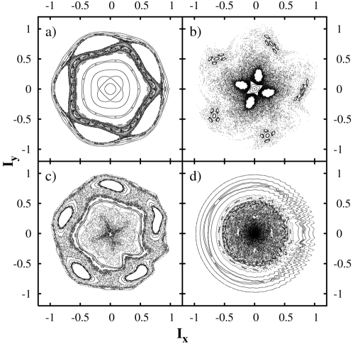
Figure 3: Poincaré map in the polar normalized action–angle variables: a) $k_{z}=0$, b) $k_{z}=2\pi/2$ km^-1, c) $k_{z}=2\pi/1$ km^-1, d) $k_{z}=2\pi/0.2$ km^-1. $I_{x}=(I/I_{s})\cos{\vartheta}$, $I_{y}=(I/I_{s})\sin{\vartheta}$, $I_{s}=I(E=0)$.

When $k_{z}$ is very small or equal to zero, ray dynamics is predominantly regular (Fig. 3a). Chaos occurs only in the isolated chaotic layer near $I=I(E_{r})$, where nondegeneracy violates. Nevertheless, inclusion of even slow vertical oscillations broaden the chaotic layer greatly, that is shown in Fig. 3b. The so-called ‘‘chaotic sea’’ emerges and chaotic diffusion in phase space becomes unbounded and global. The chaotic sea is rarely filled by points due to strong ray escaping. Such amplification of ray escaping is induced by vertical resonance (30) which affects especially the steep rays satisfying the condition RAO16

$$|p_{\text{max}}(I)|=\frac{\lambda_{z}}{\lambda_{r}}=0.2.$$ (41)

With further increasing $k_{z}$ the most steep rays exhibit the transition chaos – stability. It is shown in Fig. 3c, where the Poincaré map for the case of $k_{z}=2\pi/1.0$ km^-1 is depicted. Now the chaotic sea is separated into two parts, the internal layer and the external one (Fig. 3c). Both these layers are restricted by invariant curves. Complete stabilization of the steep rays takes place in the case of $k_{z}=2\pi/0.2$ km^-1 (Fig. 3d). With that, the internal chaotic layer occupies entirely the range of small values of the action.

In Fig. 4 fragments of three ray trajectories with $k_{z}$, varying from $2\pi/2.0$ km^-1 to $2\pi/0.2$ km^-1, are shown. Initial conditions and other parameters of the sound channel are the same for all trajectories. All the rays are launched from the channel axis with the same starting momentum $p(r=0)=0.03$. The ray with $k_{z}=2\pi/2.0$ km^-1 is completely stable, that is in agreement with Fig. 3b. In the case of $k_{z}=2\pi/1$ km^-1 the ray belongs to the internal chaotic layer and, therefore, is chaotic (this case corresponds to Fig. 3c), but its irregular behavior is not so apparent, as that of the ray with $k_{z}=2\pi/0.2$ km^-1. In the latter case the ‘‘elevating’’ effect takes place – the ray, being trapped into a microchannel near the lower turning point, leaves it only near the upper turning point. The action of an ‘‘elevated’’ ray insreases appreciably.

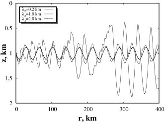
Figure 4: Ray trajectories with different values of vertical wavenumber of the perturbation $k_{z}$. All the rays are launched from the axis of the waveguide with one and the same starting momentum $p(r=0)=0.03$

The qualitative description, being provided by the Poincaré maps, enables to explore the properties of the wave field in the time – depth plain at a receiver, the so-called timefront. Timefronts were the main measurable characteristics in the recent long-range experiments Spind .

Chaotic dynamics of rays leads to divergence of their trajectories and, therefore, arrival times of chaotic rays with close launching angles can be very different. Besides that, topology of the Poincaré maps (Fig. 3) shows that only the rays with certain values of the action perform chaotic motion, whereas the rest part of phase space corresponds to stable rays. Therefore, arrival time spreading is significant only in some finite segments of a timefront of a received pulse.

We computed timefronts with different values of $k_{z}$. Each timefront is modeled as superposition of arrivals of 50000 rays started from the channel axis. The initial momentum $p$ is uniformly distributed in the interval $[-p_{\text{max}}:p_{\text{max}}]$, where $p_{\text{max}}=p(E=0)\simeq 0.22$. The timefronts for $k_{z}=0$ and $k_{z}=2\pi/0.2$km^-1 are presented in Fig. 5. In the case $k_{z}=0$ the time spreading is weak. There are two prominent gaps and densely filled region amid them in arrival pattern, those correspond to the horizontal resonance with $l=1$ and $m=5$. Such gaps are absent in the case of $k_{z}=2\pi/0.2$km^-1, that is connected with suppressing of horizontal resonance in the regime of fast vertical oscillations of a sound-speed perturbation. In this case the final portion of the pulse is chaotic and unresolved, that is a consequence of strong chaos of near-axial rays with small values of the action.

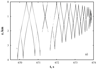
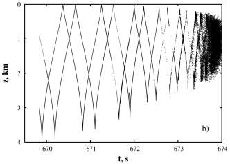
Figure 5: Timefront of a received pulse at the range 1000 km in the periodically perturbed waveguide: a) $k_{z}=0$, b) $k_{z}=2\pi/0.2$km^-1.

IV Random sound-speed perturbation

Internal waves in the deep ocean are known to have continuous spectrum and must be considered rather as a stochastic process than a deterministic one. So the following question arises: in what extent results of the previous section can be referred to acoustic propagation in a randomly perturbed sound channel? Our goal now is to investigate how ray dynamics depends on the vertical scale of random longitudinal sound-speed variations.

In the present section we consider the sound-speed perturbation given in the form

$$\delta c(z,r)=\varepsilon c_{0}\frac{z}{B}\,e^{-2z/B}\xi(z,r),$$ (42)

where a random function $\xi(z,\,r)$ is expressed as

$$\xi(z,r)=\cos{\left[\pi\left(ue^{-vz}+\sqrt{2}A_{\xi}\tilde{\xi}(r)\right)\right]}\tilde{\xi}(r),$$ (43)

where $A=1$, $v=1$ km^-1 and $\tilde{\xi}(r)$ is a random function with normalized first and second moments

$${\left<\tilde{\xi}(r)\right>}=0,\quad{\left<\tilde{\xi}^{2}(r)\right>}=\frac{1}{2}.$$ (44)

A function $\tilde{\xi}(r)$ is modeled as a sum of 10000 randomly-phased harmonics with wavenumber distributed in the range from $2\pi/100$ km^-1 to $2\pi/1$ km^-1. Spectral density of $\tilde{\xi}(r)$ decays with $k$ as $k^{-2}$. Single realizations of the perturbation with $u=5$ and $u=20$ are presented in Fig. 6.

Figure 6: Sound-speed perturbation vs depth: a) $u=5$, b) $u=20$.

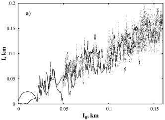
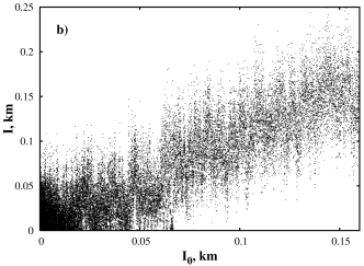
Figure 7: Ray action at the range 1000 km as a function of its initial value in the randomly perturbed waveguide. a) $u=5$, b) $u=20$.

We integrated numerically the ray equations with the parameter $u$ varying from 5 to 20. Figure 7 represents the ray action at the range 1000 km as the function of the starting action $I_{0}$. In the case of slowly varying vertical structure with $u=5$ (upper plot) chaoticity grows gradually with increasing $I_{0}$. Flat rays don’t perform extreme sensitivity to initial conditions and dependence is continuous in the range of small $I_{0}$. Isolated continuous pieces belong to bundles formed by stable or weakly chaotic rays with close launching angles and converging travel times, namely coherent clusters Chaos . Coherent clusterization is a sort of cooperative effects in randomly-driven nonlinear Hamiltonian systems Arxiv . Creation of coherent clusters results from the resonant interaction of unperturbed ray motion with low-frequency components of a random perturbation. In point of fact coherent clusters can be considered as counterparts of islands of stability. Continuous pieces melt with increasing $I_{0}$ and the dependence $I(I_{0})$ become almost irregular, that attests ray divergence and chaos.

In spite of the case $u=5$ there are no any remarkable coherent clusters in the case of $u=20$. The dependence $I(I_{0})$ is chaotic for all values of the starting action. It should be noted that the region of small values of the action is more fuzzy than the region of large ones. Moreover, spreading of values of the action depends slightly on $I_{0}$ for steep rays, that implies homogeneous chaotic diffusion. According to Virovlyansky Viro ; Radio , if ray diffusion in phase space is homogeneous and can be treated as a Wiener process, early arrivals are expected to be well-resolved. This statement is confirmed by the timefronts computed with $u=5$ and $u=20$ (Fig. 8). If $u=5$ (upper plot) all the arrivals are well resolved, but their distribution is nonuniform: coherent clusters, looking as concentrations of plotting points with extremely small time spreading, alternate with rarely filled regions. On the other hand, all the timefront branches are fuzzy in the case of $u=20$. Time spreading, however, abates with decreasing the arrival time and is less than distance between neighboring branches in the early portion of the pulse. Locations of branches and the envelope of a timefront in the early portion are coincide with ones for the unperturbed problem. As long as these characteristics can be considered as ‘‘marks’’ of environment, those are relevant for the long-range acoustic thermometry Worc ; Mikh or monitoring of the large-scale ocean variability RAO15 .

The stability of early portion of a received pulse can be clarified in the same way as that it has done in the case of the periodic perturbation in the Section III. Correlation length of sound-speed variations along a ray path is given by the formula BrV

$$L=\left[\frac{1-p^{2}}{L_{r}^{2}}+\frac{p^{2}}{L_{z}^{2}}\right]^{-1/2},$$ (45)

where $L_{r}$ and $L_{z}$ are the horizontal and the vertical correlation length scales of sound-speed variations, respectively. If $L_{z}$ is small enough, correlation length is expressed as $L=L_{z}/p$ and, therefore, is minimal for steep rays. Thus, if the criterion (37), being expressed as

$$\left|\frac{dV}{dz}\right|\ll\left|k_{z}V\right|,\quad\omega\ll\frac{|p|}{L_{z}},$$ (46)

is satisfied, fast oscillations of the perturbation suppress each other and diffusion in phase space weakens, that reveals itself in diminishing time spreads in the early portion of a received pulse.

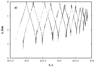
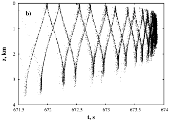
Figure 8: Timefront of a received pulse at the range 1000 km in the randomly perturbed waveguide: a) $u=5$, b) $u=20$.

V Summary and discussion

In the present paper we have investigated in what manner stability of rays in an underwater sound channel depends on the vertical scale of a sound-speed inhomogeneity induced by internal waves. The main result is that fast depth oscillations of a sound-speed perturbation can lead to stability of the steep rays forming early portion of a received pulse in experiments. We found that a ray can be captured in resonance with vertical sound-speed variations, which we call as vertical resonance. If the length scale of vertical variations is large enough, vertical resonance enforces strong chaos and escaping of steep rays.

Our results rely on the ray approximation without referring to the pulse characteristics, but we suggest that they can be worthwhile for understanding some features of the propagation of a monochromatic acoustic wave. This suggestion is mainly based on the results presented in the recent paper Hege , there the task of the ray/wave method correspondence was studied. As was reported in Hege , improving of ray predictions requires to smooth those features of internal wave fine structure, which have vertical length scale less than the threshold of wavefield responsibility defined by the formula

$$\lambda_{\text{min}}=\frac{c_{0}}{\Omega\tan\phi_{\text{max}}},$$ (47)

where $\Omega$ is the career frequency and $\tan\phi_{\text{max}}$ is the maximal grazing angle. For $\Omega=75$ Hz this scale of roughly of $110$ m. On the other hand, we have found ray dynamics to be very sensitive to the fine structure of the internal wave field, that implies the arrival pattern to change with varying frequency. For instance, the early portion of a received pulse can lose stability at very low frequencies, when the threshold given by (47) is large. This seems to associate the anomalous low-frequency sound attenuation Vadov with strong ray escaping.

However, there are many questions concerning structure of late arrivals. First, $\lambda_{\text{min}}$ is large enough for flat rays, so they are expected to be insensitive to the small vertical features of the background sound-speed profile. Second, it is impossible to use geometrical acoustics to describe the propagation along the axis of a waveguide due to multiple caustics GFP . On the other hand, forming of coherent ray clusters should explain the well-resolved coherent late arrivals which were observed at 28 Hz in the AST experiment Wage . So the following question arises: in what extent complicated structure of the arrival final is linked with ray chaos? This topic will be aim of our future research.

Appendix

The action variable for the rays with $E<E_{r}$ is given by the formula

$$I=\frac{b}{a}\left(\frac{\mu+\gamma}{2}-\sqrt{\mu\gamma-\frac{2E}{b^{2}}}\right).$$ (48)

The respective expression for the angle variable is the following

$$\vartheta=\pm\frac{\pi}{2}\mp\arcsin{\frac{\mu+\gamma-(2\mu\gamma-4E/b^{2})\,e^{az}}{Q}},$$ (49)

where the quantity Q is given by the formula

$$Q=\sqrt{(\mu-\gamma)^{2}+\frac{8E}{b^{2}}}.$$ (50)

The upper and the lower signs in (49) correspond to the case of $p>0$ and to the case $p\leq 0$, respectively. The action and the angle for surface-bounce rays are given by the following formulas

$$I=\frac{p(z=0)}{\pi a}+\frac{b}{a}\Biggl{(}\frac{\mu+\gamma}{4}-\frac{\mu+\gamma}{2\pi}\times\\ \times\arcsin{\dfrac{\mu+\gamma-2}{Q}}-\frac{\pi-\theta_{r}}{\pi}\sqrt{\mu\gamma-\frac{2E}{b^{2}}}\Biggr{)},$$ (51)

$$\vartheta=\frac{\pi}{\pi-\vartheta_{r}}\Biggl{[}\frac{\pi}{2}-\vartheta_{r}-\\ -\arcsin{\dfrac{\mu+\gamma-(2\mu\gamma-4E/b^{2})\,e^{az}}{Q}}\Biggr{]},\quad p\geq 0,\\ \vartheta=\frac{\pi}{\pi-\vartheta_{r}}\Biggl{[}\frac{\pi}{2}+\\ +\arcsin{\dfrac{\mu+\gamma-(2\mu\gamma-4E/b^{2})\,e^{az}}{Q}}\Biggr{]},\quad p<0.$$ (52)

In (51)–(52) we used the notation

$$\vartheta_{r}=\frac{\pi}{2}-\arcsin\left[\frac{\mu+\gamma-2\mu\gamma+4E/b^{2}}{Q}\right].$$ (53)

Under reflections, the ray momentum is given by the formula

$$p(z=0)=\sqrt{2E-b^{2}(\mu-1)(\gamma-1)}.$$ (54)

The inverse transformation for the rays, propagating without reflections from the surface, is expressed as follows

$$z(I,\,\vartheta)=\dfrac{1}{a}\ln{\dfrac{a^{2}b^{2}\,\left(\mu+\gamma-Q\cos{\vartheta}\right)}{2\omega^{\prime 2}}},$$ (55)

$$p(I,\,\vartheta)=\dfrac{\omega\,Q\sin{\vartheta}}{a\left(\mu+\gamma-Q\cos{\vartheta}\right)},$$ (56)

where

$$\omega^{\prime}(I)=\frac{ab\,(\mu+\gamma)}{2}-a^{2}I.$$ (57)

The quantity $\omega^{\prime}$ coincides with spatial frequency of ray oscillations $\omega$ for the rays propagating without reflections from the surface. Position and momentum of the surface-bounce rays are expressed as follows

$$z(I,\,\vartheta)=\dfrac{1}{a}\ln\dfrac{a^{2}b^{2}\left[\mu+\gamma+Q\cos{\left(\frac{\pi-\vartheta_{r}}{\pi}(\vartheta+\pi)\right)}\right]}{2\omega^{\prime 2}},$$ (58)

$$-\pi\leq\vartheta\leq 0,$$

$$z(I,\,\vartheta)=\dfrac{1}{a}\ln\dfrac{a^{2}b^{2}\left[\mu+\gamma-Q\cos{\left(\frac{\pi-\vartheta_{r}}{\pi}\vartheta+\vartheta_{r}\right)}\right]}{2\omega^{\prime 2}},$$

$$0\leq\vartheta\leq\pi.$$

$$p(I,\,\vartheta)=\dfrac{\omega^{\prime}Q\sin{\left(\frac{\pi-\vartheta_{r}}{\pi}(\vartheta+\pi)\right)}}{a\left[\mu+\gamma+Q\cos{\left(\frac{\pi}{\pi-\vartheta_{r}}(\vartheta+\pi)\right)}\right]},$$ (59)

$$-\pi\leq\vartheta\leq 0,$$

$$p(I,\,\vartheta)=\dfrac{\omega^{\prime}Q\sin{\left(\frac{\pi-\vartheta_{r}}{\pi}\vartheta+\vartheta_{r}\right)}}{a\left[\mu+\gamma-Q\cos{\left(\frac{\pi-\vartheta_{r}}{\pi}\vartheta+\vartheta_{r}\right)}\right]},$$

$$0\leq\vartheta\leq\pi.$$

References

- (1) A.V. Chigarev and Yu.V. Chigarev, Akust. Zh. 24, 765 (1978) [Sov. Phys. Acoust. 24, 432 (1978)].
- (2) S.S. Abdullaev and G.M. Zaslavsky, Zh. Eksp. Teor.Fiz. 80, 524 (1981) [Sov. Phys. JETP. 53, 265 (1981)].
- (3) D.R. Palmer, M.G. Brown, F.D. Tappert, and H.F. Bezdek, Geophys. Res. Let. 15, 569 (1988).
- (4) S.S. Abdullaev and G.M. Zaslavsky, Usp. Fiz. Nauk 161, 1 (1991) [Sov. Phys. Usp. 34, 645 (1991)].
- (5) M.G. Brown, J.A. Colosi, S. Tomsovic, A.L. Virovlyansky, M.A. Wolfson, and G.M. Zaslavsky, J. Acoust. Soc. Am. 113, 2533 (2003).
- (6) W.H. Munk and C. Wunsch, Deep-Sea Res. 26, 123 (1979).
- (7) J.L. Spiesberger, J. Acoust. Soc. Am. 77, 83. (1985).
- (8) J.L. Spiesberger J.L., J. Geophys. Res. 96. 4869 (1991).
- (9) V.A. Akulichev, V.P. Dzyuba, P.V. Gladkov, S.I. Kamenev, and Yu.N. Morgunov, in Theoretical and Computational Acoustics, edited by Er-Chang Shang, Qihu Li, and T.F. Gao (World Scientific, Singapore, 2002).
- (10) R.C. Spindel, J. Na, P.H. Dahl, S. Oh, C. Eggen, Y.G. Kim, V.A. Akulichev, and Yu.N. Morgunov, IEEE J. Ocean. Engin. 28, 297 (2003).
- (11) V.A. Akulichev, V.V. Bezotvetnykh, E.A. Voitenko, S.I. Kamenev, A.P. Leont’ev, and Yu.N. Morgunov, Acoustical Physics 50, 493 (2004).
- (12) K.B. Smith, M.G. Brown, and F.D. Tappert, J. Acoust. Soc. Am. 91, 1939 (1992).
- (13) K.B. Smith, M.G. Brown, and F.D. Tappert, J. Acoust. Soc. Am. 91, 1950 (1992).
- (14) F.D. Tappert and Xin Tang, J. Acoust. Soc. Am. 99, 185 (1996).
- (15) P.F. Worcester and R.C. Spindel, J. Acoust. Soc. Am. 117, Pt. 2, 1499 (2004).
- (16) P.F. Worcester, B.D. Cornuelle, M.A. Dzieciuch, W.H. Munk, B.M. Howe, J.A. Mercer, R.C. Spindel, J.A. Colosi, K. Metzger, T.J. Birdsall, and A.B. Baggeroer, J. Acoust. Soc. Am. 105, 3185 (1999).
- (17) F.J. Beron-Vera, M.G. Brown, J.A. Colosi, S. Tomsovic, A.L. Virovlyansky, M.A. Wolfson, and G.M. Zaslavsky, J. Acoust. Soc. Am. 114, 1426 (2003); e-print arXiv:nlin.CD/0301026.
- (18) D.V. Makarov, M.Yu. Uleysky, and S.V. Prants, Chaos 14. 79 (2004); e-print arXiv:nlin.CD/0306056.
- (19) D.V. Makarov, S.V. Prants, and M.Yu. Uleysky, Doklady Earth Science 382, 106 (2002).
- (20) D.V. Makarov, Nonlinear dynamics of rays in a range-dependent underwater sound channel, Ph.D. dissertation [in Russian] (V.I.Il‘ichev Pacific Oceanological Institute, Vladivostok, 2004).
- (21) J.D. Meiss, Chaos 7. 139 (1997).
- (22) M.V. Budyansky, M.Yu. Uleysky, and S.V. Prants, Physica D 195. 369 (2004); e-print arXiv nlin.CD/0208032.
- (23) Soo-Young Lee, Sungwan Rim, Jung-Wan Ryu, Tae-Yoon Kwon Muhan Choi, and Chil-Min Kim, Phys.Rev.Lett. 93. 164102 (2004); e-print arXiv:nlin.CD/0403025 (2004).
- (24) L.D. Landau and E.M. Lifshitz, Mechanics (Pergamon, London, 1976).
- (25) I.P. Smirnov, A.L. Virovlyansky, and G.M. Zaslavsky, Phys. Rev. E 64, 1 (2001).
- (26) B.V. Chirikov, Phys. Rep. 52, 265 (1979).
- (27) D.V. Makarov, M.Yu. Uleysky, and S.V. Prants, Tech.Phys. Lett. (2003).
- (28) F.J. Beron-Vera and M.G. Brown, J. Acoust. Soc. Am. 114, 123 (2003); e-print arXiv:nlin.CD/0208038.
- (29) A.L. Lichtenberg and M.A. Lieberman, Regular and Stochastic Motion (Springer, New York, 1992).
- (30) G.M. Zaslavsky, Physics of Chaos in Hamiltonian Systems (Academic Press, Oxford, 1998).
- (31) D.V. Makarov and M.Yu. Uleysky, Proceedings of the X-th L.M. Brekhovskikh‘s Conference [in Russian] 134 (2004).
- (32) S. Rahav, I. Gilary, and S. Fishman. Phys. Rev. A 68, 013820 (2003).
- (33) M.Yu. Uleysky. Study of statistical properties of chaotic nonlinear oscillations in Hamiltonian systems, Ph.D. dissertation [in Russian]. (V.I.Il‘ichev Pacific Oceanological Institute, Vladivostok, 2005).
- (34) M.Yu. Uleysky and D.V. Makarov, to be published in Proceedings of the XVI-th Session of Russian Acoustical Society (2005).
- (35) D.V. Makarov, M.Yu. Uleysky, M.V. Budyansky and S.V. Prants, e-print arXiv:nlin.CD/0507010 (2005).
- (36) A.L. Virovlyansky, J. Acoust. Soc. Am. 113, 2523 (2003).
- (37) A.L. Virovlyansky, Izv. VUZ.Radiofiz. 146, 555 (2003).
- (38) P.N. Mikhalevsky, A. Gavrilov, and A.B. Baggeroer. IEEE J.Ocean.Engin. 24, 183 (1999).
- (39) D.V. Makarov, M.Yu. Uleysky, and M.Yu. Martynov. Proceedings of the XV-th Session of Russian Acoustical Society 140 (2004).
- (40) M.G. Brown and J. Viechnicky, J. Acoust. Soc. Am. 104, 2090 (1999).
- (41) K.C. Hegewisch, N.R. Cerruti, and S. Tomsovic, 117, Pt. 2, 1582 (2004); e-print arXiv:physics/0312150 (2003).
- (42) R.A. Vadov, Acoustical Physics 46, 544 (2000).
- (43) N.S. Grigorieva, G.M. Fridman, and D.R. Palmer. J. Comp.Acoust. 12, 355 (1999).
- (44) K.E. Wage, M.A. Dzieciuch, P.F. Worcester, B.M. Howe, and J.A. Mercer. 117, Pt. 2, 1565 (2004).