Understanding widely scattered traffic flows, the capacity drop, platoons, and times-to-collision as effects of variance-driven time gaps

Abstract

We investigate the adaptation of the time headways in car-following models as a function of the local velocity variance, which is a measure of the inhomogeneity of traffic flow. We apply this mechanism to several car-following models and simulate traffic breakdowns in open systems with an on-ramp as bottleneck. Single-vehicle data generated by several ’virtual detectors’ show a semi-quantitative agreement with microscopic data from the Dutch freeway A9. This includes the observed distributions of the net time headways and times-to-collision for free and congested traffic. While the times-to-collision show a nearly universal distribution in free and congested traffic, the modal value of the time headway distribution is shifted by a factor of about two in congested conditions. Macroscopically, this corresponds to the ’capacity drop’ at the transition from free to congested traffic. Finally, we explain the wide scattering of one-minute flow-density data by a self-organized variance-driven process that leads to the spontaneous formation and decay of long-lived platoons even for deterministic dynamics on a single lane.

I Introduction

One of the open questions of traffic dynamics is a microscopic understanding of the observed wide variations in the time-headway distributions Tilch and Helbing (2000); Neubert et al. (1999) that are closely related to the wide scattering of flow-density data in the congested regime Kerner and Rehborn (1996); Nishinari et al. (2003), see, e.g., Refs. Kerner (2004); Helbing (2001) for an overview. Apart from their wide variations, the average values of the time headways depend strongly on the traffic density. For congested traffic, the modal value, i.e., the value where the distribution has its maximum, is larger by a factor of about 2 compared to free traffic. Figure 1(a) shows a typical example obtained from single-vehicle detector data of the Dutch freeway A9 from Haarlem to Amsterdam.

With the increasing availability of single-vehicle data Tilch and Helbing (2000); Neubert et al. (1999); Knospe et al. (2002), further statistical properties of traffic became the subject of investigation such as the velocity variance as a function of the traffic density Treiber et al. (1999), or the distribution of the times-to-collision (TTC), which plays an important role for traffic safety Minderhoud and Bovy (2001); Hirst and Graham (1997).

In this paper, we therefore propose a variance-driven adaptation mechanism, according to which drivers increase their safety time gaps $T$ when the local traffic dynamics is unstable or largely varying. This adaptation is, e.g., reflected in the empirically observed increase of the variation coefficient $V=\theta/\bar{v}$ and offers a safety-oriented interpretation of the capacity drop, i.e., the significant reduction of traffic flow when it becomes unstable Hall and Agyemang-Duah (1991); Daganzo et al. (1999); Kerner and Rehborn (1997).

Variance-driven time headways can also qualitatively explain the distribution of times-to-collision, which is surprisingly invariant with respect to density changes (compared to distance, time gap, or velocity distributions). Times-to-collision are, therefore, not only an interesting measure for traffic safety, but also a meaningful variable of behaviorally-oriented traffic models based on the physical approach of invariants Treiber et al. (2005); Lenz et al. (1998).

The variance-driven increase of the safety time gap $T$ may also be seen as an alternative to a frustration-driven increase of $T$ after a long time in congested traffic Treiber and Helbing (2003); Tilch and Helbing (2000); Neubert et al. (2000); Lei . Moreover, it potentially overcomes the criticism of traffic models with a fundamental diagram by Kerner Kerner (2004), as it causes a pronounced platooning effect when traffic flow is perturbed or unstable. This guarantees a wide gap distribution which is the main prerequisite to reproduce the wide scattering of flow-density data in congested traffic Nishinari et al. (2003); Kerner and Rehborn (1996).

Previous explanations of the wide scattering of flow-density data include stochastic effects Gipps (1981); Brackstone and McDonald (1999), and sustained non-equilibrium states caused by dynamic instabilities such as stop-and-go traffic Treiber and Helbing (2003). Stochastic terms are included in most cellular-automaton traffic models Nagel and Schreckenberg (1992); Knospe et al. (2004) and also in some car-following models, e.g., in the Gipps-model Gipps (1981) or in recent car-following models proposed by Kerner Kerner and Klenov (2002) or Wagner Wagner (2004). Another explanation of the scattering is based on the heterogeneity of vehicles (such as cars and trucks) and driving styles (such as defensive or aggressive) Treiber and Helbing (1999); Daganzo et al. (1999); Helbing and Treiber (2002). However, while all these effects can possibly account for the observed variations of time headways and times-to-collision, at least for a given traffic density, the scattering of flow-density data would be smaller than observed due to the averaging implied in aggregating single-vehicle data to, e.g., one-minute data Nishinari et al. (2003).

In the next section, we will introduce the mechanism of variance-driven time headways (VDT) in terms of a ’meta-model’ which can be applied to a wide range of car-following models. Section III introduces a general method to add fluctuations to car-following models. In Sec. IV, we apply the VDT mechanism to three microscopic traffic models and compare ’virtual-detector data’ directly with empirical findings. We found that this simple mechanism can semiquantitatively explain all the microscopic and macroscopic empirical findings mentioned above. In the concluding Sec. V, we discuss the effects of the VDT mechanism in terms of a spontaneous formation and decay of vehicle platoons, and point to applications in the field of traffic control and driver-assistance systems.

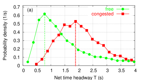
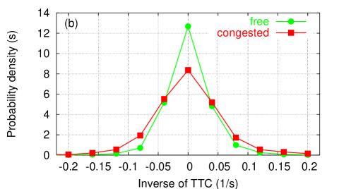
Figure 1: Empirical statistical properties of cars following any kind of vehicle obtained from single-vehicle data from the left lane of the Dutch freeway A9 at a detector cross section 1.0 km upstream of an on-ramp. (a) Net time headway according to Eq. (18); (b) Inverse times-to-collision according to Eq. (19); (c) Variance coefficient $V_{n}$ according to Eq. (2), as a function of the density. In (a) and (b), the data set for ’free traffic’ includes all single-vehicle data where the one-minute average of velocities was above 20 m/s, and the traffic flow above 1000 vehicles/h. ’Congested traffic’ includes all data where the one-minute average of the velocities was below 15 m/s.

II Variance-driven adaptation of the time headway

We will formulate the variance-driven time headways (VDT) model in terms of a meta-model to be applied to any car-following model where the time headway $T_{0}$ for equilibrium traffic can be expressed by a model parameter or a combination of model parameters.

The basic assumption of the VDT is that smooth traffic flow allows for lower values of the time headway than disturbed traffic flow where the actual time headway

$$T=\alpha_{T}T_{0}$$ (1)

is increased with respect to $T_{0}$ by a factor $\alpha_{T}\geq 1$. Furthermore, we characterize disturbed traffic flow (such as stop-and-go traffic) by relatively high values of the velocity differences between following vehicles. Since a driver in vehicle $\alpha$ must assess the heterogeneity of traffic flow in situ, any measure for the heterogeneity may only depend on the immediate environment. One of the simplest measure satisfying this requirement is the local variation coefficient

$$V_{n}=\frac{\sqrt{\theta_{n}}}{\bar{v}_{n}}$$ (2)

where the local velocity average

$$\bar{v}_{n}=\frac{1}{n}\sum\limits_{i=0}^{n-1}v_{\alpha-i},$$ (3)

and the local variance

$$\theta_{n}=\frac{1}{n-1}\sum\limits_{i=0}^{n-1}(v_{\alpha-i}-\bar{v}_{n})^{2}$$ (4)

are calculated from the own velocity $v_{\alpha}$ and the velocities of the $(n-1)$ predecessors $(\alpha-i),i=1,\ldots,n-1$. For the sake of simplicity we will skip the vehicle index $\alpha$ here, and in all subsequent equations. In this work, we will set $n=5$ in most cases, i.e., the adaptation of the drivers is assumed to depend on the own velocity and the velocities of the four nearest vehicles in front.

This quantity can be empirically determined if single-vehicle data are available. Figure 1(c) shows an example for the Dutch freeway A9 between Haarlem and Amsterdam. Notice that, for a given local density $\rho$, the variation coefficient $V_{n}=\sqrt{A}$ is related to the variance prefactor $A(\rho)$ introduced in the macroscopic gas-kinetic-based traffic (GKT) model Treiber et al. (1999).

Let us now assume that the multiplication factor $\alpha_{T}$ of the time headway is adapted instantaneously to a traffic situation according to

$$\alpha_{T}=\min\left(1+\gamma V_{n},\alpha_{T}\sup{max}\right).$$ (5)

Here, $\alpha_{T}\sup{max}$ denotes the maximum multiplication factor for the time headway for traffic flows of maximum unsteadiness, and

$$\gamma=\frac{1}{T_{0}}\frac{{\rm d}T}{{\rm d}V_{n}}$$ (6)

the sensitivity of the time headway to increasing velocity variations.

In summary, Eqs. (2) - (5) imply that the necessary time headway for safe driving depends on the velocity variance of the surrounding traffic. This proposition of variance-driven time headways (VDT) can be applied to any time-continuous car-following model in which the time headway can be expressed by a model parameter or a combination of parameters. Some examples are the optimal-velocity model (OVM) Bando et al. (1995), the velocity-difference model (VDIFF) Jiang et al. (2001), the intelligent-driver model (IDM) Treiber et al. (2000), or the Gibbs model Gipps (1981).

The VDT has three parameters, namely the number $n$ of vehicles used to determine the local velocity variance, the maximum multiplication factor $\alpha_{T}$ by which the time headway is increased compared to perfectly smooth traffic, and the sensitivity $\gamma$. For the special case $n=2$, the VDT acceleration depends only on the velocity difference to the immediate predecessor, i.e., one obtains a simple car-following model depending only on the immediate predecessor (at least, if this is the case for the underlying car-following model). However, the model yields more realistic results for a larger number of vehicles, therefore we will assume $n=5$ in all simulations (see Table 1). Larger values for $n$ will not change the dynamics significantly.

The parameters $\alpha_{T}$ and $\gamma$ can be determined from empirical data of the time-headway distribution for free and congested traffic, and from the observed maximum variation coefficient $V_{n}\sup{max}$. Figure 1 shows these data for the Dutch freeway A9 from Haarlem to Amsterdam Tilch and Helbing (2000). Figure 1(a) shows that the locations of the maxima (modal values) of the time-headway distributions for free and congested traffic differ by a factor of about two. We therefore set $\alpha_{T}\sup{max}=2$ in all simulations. The parameter $\gamma$ can be determined by the approximate relation

$$\gamma\approx\frac{\alpha_{T}\sup{max}-1}{V_{n}\sup{max}}.$$ (7)

From Fig. 1(c) we see that $V_{n}\sup{max}$ is slightly below 0.2, so we set $\gamma=5$ in all simulations.

Parameter	Value
Number $n$ of vehicles for determining $\theta$	5
Time-headway multiplication factor
in unsteady traffic $\alpha_{T}\sup{max}$	2.2
Sensitivity $\gamma$	4.0

Table 1: Model parameters of the VDT approach used throughout this paper for all simulated car-following models. The strength of the acceleration noise (cf. Sec. III) was set to $0.1\,\text{m}^{2}/\text{s}^{3}$.

III Acceleration noise

Fluctuating forces in microscopic traffic models are used to globally describe all influences that are not modeled explicitly such as imperfect estimation capabilities Treiber et al. (2005), lack of attention, or simply the fact that drivers do not always react identically to a given traffic situation. Fluctuation terms are part of nearly all cellular automata (the most popular example being the Nagel-Schreckenberg model Nagel and Schreckenberg (1992) and models derived from it Chowdhury et al. (2000)), but are less commonly used in time-continuous car-following models.

Since the VDT is essentially based on fluctuations of the velocity, it is to be expected that purely deterministic underlying models yield unrealistic results due to the lack of an initial source triggering the fluctuations. Therefore, we consider additional acceleration fluctuations when applying the VDT to a deterministic model.

For simplicity, we will just add a white (independent and $\delta$-correlated) noise term Helbing and Treiber (2003) to the deterministic car-following acceleration $a\sup{(det)}_{\alpha}$ according to

$$\dot{v}_{\alpha}=a\sup{(det)}_{\alpha}(t)+\sqrt{Q}\,\xi_{\alpha}(t).$$ (8)

Here, $Q$ denotes the fluctuation strength (cf. Table 1), and the white noise $\xi(t)$ is assumed to be unbiased and $\delta$-correlated:

$$\mbox{$\langle\xi_{\alpha}\rangle$}=0,\ \ \mbox{$\langle\xi_{\alpha}(t)\xi_{\beta}(t^{\prime})\rangle$}=Q\delta_{\alpha\beta}\delta(t-t^{\prime}).$$ (9)

The Kronecker symbol $\delta_{\alpha\beta}$ is 1, if $\alpha=\beta$ and zero otherwise, while the Dirac function $\delta(t)$ is defined by $\int_{-\infty}^{\infty}\delta(t^{\prime})\,dt^{\prime}=1$ and $\delta(t)=0$ for $t\neq 0$. To clarify the effects of the fluctuation term on the velocity, we note that

• in the absence of a deterministic acceleration, Eq. (8) leads to velocities $v_{\alpha}(t)$ fluctuating stochastically around the initial velocity $v_{\alpha}(t_{0})$ with a linearly-in-time increasing variance (random walk),

  $$\theta_{\alpha}=Q(t-t_{0}),$$ (10)

• under the linearized deterministic (relaxational) dynamics $a\sup{det}_{\alpha}=(v_{0}-v)/\tau$ (where $v_{0}$ is the desired velocity, $v$ the actual velocity, and $\tau$ the acceleration relaxation time), the velocity variance of the stationary state is given by the fluctuation-dissipation result Gardiner (1990)

  $$\theta=Q\tau.$$ (11)

In the explicit numerical velocity update from time $t$ to $t+\delta t$,

$$v_{\alpha}(t+\delta t)=v_{\alpha}(t)+a_{\alpha}\sup{det}\delta t+\eta_{t}\sqrt{Q\delta t},$$ (12)

we have implemented the stochastic term by the additive contribution $\eta_{t}\sqrt{Q\delta t}$, where the $\{\eta_{t}\}$ are statistically independent realizations of Gaussian distributed random numbers with zero mean and unit variance Gardiner (1990).

The velocity update according to (12) is numerically consistent in the stochastic sense. More precisely, we have considered the ’numerical’ velocity distribution function $F\sup{num}(v,t)=\mbox{Prob}(v_{\alpha}(t)\leq v)$ obtained from many simulations with different seeds for the pseudo-random number generator at a given time $t$. We have then compared the numerical distribution function with the theoretical distribution $F(v,t)=\int_{-\infty}^{v}dv^{\prime}P(v^{\prime},t)$ where $P(v,t)$ is the solution to the Fokker-Planck equation corresponding to Eq. (8),

$$\frac{\partial P(v_{\alpha},t)}{\partial t}+a_{\alpha}\sup{(det)}\frac{\partial P}{\partial v_{\alpha}}=\frac{Q}{2}\frac{\partial^{2}P}{\partial v_{\alpha}^{2}}.$$ (13)

It turned out that the deviations between $F\sup{num}(v,t)$ and $F(v,t)$ are of the order ${\cal O}(\delta t)$. Notice that this means that, for sufficiently small time steps $\delta t$, the result is independent from $\delta t$ and agrees with the analytic solution to the stochastic differential equation (8).

We have checked this for the random walk and linear relaxation scenarios mentioned above and found a very good agreement between the numerical results from the update scheme (12) and the analytical results (10) and (11), respectively. (see Ref. Helbing and Treiber (2003) for a more detailed discussion).

In summary, Eqs. (8) - (12) can be considered as a general approach to add acceleration noise to time-continuous deterministic car-following models. Clearly, $\delta$-correlated noise terms are unrealistic in many respects. Therefore, we have also simulated more realistic time-correlated and multiplicative noise, which clearly describes the human origins of acceleration noise better Treiber et al. (2005), but we found no qualitative difference.

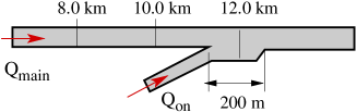
Figure 2: Simulated infrastructure and positions of virtual detectors. The units of locations are measured in kilometers.

IV Simulation results

In the following, we will apply the VDT to three car-following models, namely the intelligent-driver model (IDM) Treiber et al. (2000), the optimal-velocity model (OVM) Bando et al. (1995), and the velocity-difference model Jiang et al. (2001), which augments the OVM by a term proportional to the velocity difference. We will also simulate heterogeneous traffic consisting of a mixture of these models.

For the purpose of reference and in order to discuss the coupling to the VDT, we shortly present the model equations, i.e., the acceleration functions, of these models.

The IDM acceleration $\dot{v}_{\rm IDM}(s,v,\Delta v)$ of a vehicle as a function of the (net) distance $s$ to the predecessor, the velocity $v$, and the velocity difference $\Delta v$ (positive when approaching) is given by

$$\dot{v}_{\rm IDM}=a\left[1-\left(\frac{v}{v_{0}}\right)^{4}-\left(\frac{s^{*}}{s}\right)^{2}\right]$$ (14)

with the ’desired dynamical distance’

$$s^{*}=s_{0}+vT+\frac{v\Delta v}{2\sqrt{ab}}.$$ (15)

The acceleration of the optimal-velocity and velocity-difference models is given by

$$\dot{v}_{\rm OVM}=\frac{v_{\rm opt}-v}{\tau}-\lambda\Delta v$$ (16)

where $\lambda=0$ for the OVM and the ’optimal velocity’ is given by

$$v_{\rm opt}=\frac{v_{0}}{2}\left[\tanh\left(\frac{s}{L}-\beta\right)-\tanh(-\beta)\right].$$ (17)

The coupling (1) of the VDT to the IDM is simple, since the desired time headway $T$ is already an IDM parameter. We used $T=T_{0}=0.7$ s as minimum value which can be increased up to $T=1.54$ s corresponding to $\alpha_{T}\sup{max}=2.2$ (cf. Table 1). To find an appropriate coupling of the VDT to the OVM and VDIFF models, we note that the parameter $L$ defines a typical interaction range and, consequently, the desired time headway $s/v_{\rm opt}(s)$ is essentially proportional to $L/v_{0}$ in these models. Therefore, we coupled the VDT to the OVM and the VDIFF models by setting $L=L_{0}\alpha_{T}$ with $\alpha_{T}$ according to Eq. (5).

In order to distinguish between freely moving and following vehicles, we need at least two vehicle types (’cars’ and ’trucks’) with different desired velocities $v_{0}$. For all models, we have set $v_{0}=35$ m/s for ’cars’, and $v_{0}=25$ m/s for ’trucks’ and simulated a truck percentage of 20%. Notice that $v_{0}$ is a common parameter of all three models. Because we want to introduce as little complexity as possible, we did not distinguish cars and trucks with respect to other parameters. Furthermore, we used the same vehicle length $l_{\rm veh}=5$ m for both vehicle types in all simulations.

The remaining IDM parameters are the minimum gap $s_{0}=3$ m, the acceleration $a=1\,\mbox{m/s${}^{2}$}\,$, and the comfortable deceleration $b=1.5\,\mbox{m/s${}^{2}$}\,$. For the OVM, we used the relaxation time $\tau=0.4$ s and the form factor $\beta=1$. Furthermore, we set the interaction length $L_{0}=13$ m for cars and $L_{0}=10$ m for trucks. Thus, the effective time headway is about the same for both types. For the VDIFF, we used the same values for $L_{0}$ and $\beta$ as for the OVM. Furthermore, we used $\tau=2$ s and the sensitivity coefficient $\lambda=1\,{\rm s}^{-1}$. For all models, we set the fluctuation strength $Q=0.1\,{\rm m}^{2}/{\rm s}^{3}$. For comparison, we simulated also the deterministic VDT-IDM for which the fluctuation strength is $Q=0$. The parameters were chosen such that the traffic dynamics was comparable to the Dutch freeway A9 freeway data with respect to the form of the fundamental diagram, capacity, and stability.

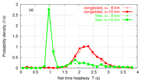
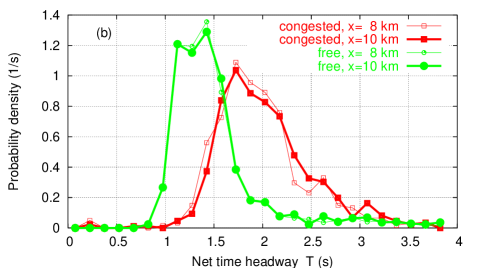
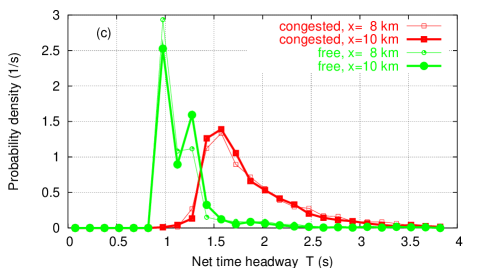
Figure 3: Distribution of the net time headways of cars following any kind of vehicle (cars or trucks) obtained from single-vehicle data of ’virtual detectors’ at various positions for simulations of the VDT with (a) the IDM; (b) the OVM; (c) the VDIFF model.

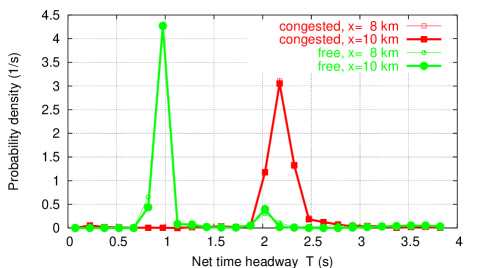
Figure 4: Distribution of the net time headways of cars for the deterministic VDT-IDM.

We have simulated a single-lane road section of total length 15 km with an on-ramp of length $L_{\rm rmp}=200$ m located at $x_{\rm rmp}=12$ km (Fig. 2) from which a constant flow of 400 vehicles/h merges to the main road. To keep matters simple, we have avoided explicit modeling of the merging of ramp vehicles to the main road. Instead, we have inserted the ramp vehicles centrally into the largest gap within the 200 m long ramp section. In order to generate a sufficient velocity perturbation in the merge area, the speed of the accelerating on-ramp vehicles at the time of insertion was assumed to be 50% of the velocity of the respective front vehicle. It turned out that the perturbations induced by the slower merging vehicles were crucial: When simulating merges with the same velocity as the main road vehicles, the onset of traffic breakdown was markedly delayed indicating the role of perturbations for traffic optimization (see Sec. V below).

We initialized the simulations with very light traffic of density $\rho=3$ vehicles/km and an initial velocity of 100 km/h. The details of the initial conditions, however, are not relevant unless they lead to an immediate breakdown of traffic flow. To generate congestion, we have increased the inflow of vehicles to the main lane linearly from 300 vehicles/h at $t=0$ s to 3000 vehicles/h at $t=2400$ s. Afterwards, we decreased the inflow linearly to 300 vehicles/h until $t=4800$ s. In case the inflow exceeded capacity, we delayed the insertion of new vehicles at the upstream boundary.

The update time step of the numerical integration scheme was $\delta t=0.05\>\mathrm{s}$ for all models. Runs with smaller time steps yielded essentially the same results.

IV.1 Time-headway distribution

Empirical investigations of single-vehicle data have shown that the distributions of net time headways differ markedly in free and congested traffic situations Tilch and Helbing (2000); Knospe et al. (2002), see Fig. 1.

To enable direct comparisons with experimental work, we have implemented ’virtual detectors’ at $x=8$ km and 10 km (cf. Fig. 2) recording the passage time $t_{\alpha}$, type (car or truck) and velocity $v_{\alpha}$ of each vehicle $\alpha$ crossing the detector. We estimated the net time headway $T_{\alpha}$ by the time interval between the passage of the rear bumper of the preceding vehicle $(\alpha-1)$ and the front bumper of the vehicle under consideration,

$$T_{\alpha}=t_{\alpha}-t_{\alpha-1}-\frac{l_{\alpha-1}}{v_{\alpha-1}}.$$ (18)

Figure 3 shows the simulated distribution of $T_{\alpha}$ for the faster vehicle type (’cars’ following any vehicle type) separately for free traffic ($v_{\alpha}>15$ m/s) and congested traffic ($v_{\alpha}\leq 12$ m/s). We have obtained the following main results:

• The modal value (location of the maximum of the probability density) of the time headway is markedly higher (about twice as high for the VDT-IDM) in congested traffic compared to free traffic.

• The values for $T_{\alpha}$ form a broad and asymmetrical distribution.

• The different underlying models, particularly deterministic and stochastic variants, yielded the same qualitative results. Remarkably, the velocity variance depends only weakly on the noise.

Notice that the VDT only prescribes that the time headway increases with the variance. The dependence of the variance (and thus the average time headway) on the traffic situation results from the traffic dynamics. Moreover, all statistical data were obtained from identical vehicles (the ’cars’). Since all cars have the same unique equilibrium relation between velocity and net distance $s$, the wide and bimodal distributions are an interesting result, particularly for the deterministic case.

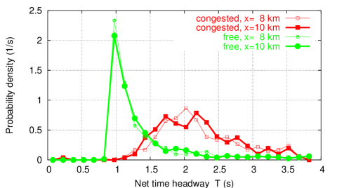
Figure 5: Distribution of time headways for the VDT with a mix of 1/3 IDM, 1/3 OVM, and 1/3 VDIFF vehicles (truck percentage 20% in each model).

Nevertheless, the peaks of the simulated distributions are higher and sharper that those in the empirical data (cf. Fig. 1) The lacking quantitative agreement in this case can be explained by the wide variation of individually preferred time headways of drivers, i.e., in the variations of the driving style Nishinari et al. (2003), which was neglected in our simulation for reasons of simplicity. To test this assumption, we have simulated a mix of all three models. The resulting time-headway distribution for congested traffic and the variance as a function of the density reproduces the observed data nearly quantitatively as shown in Fig. 5.

For the sake of simplicity, we will, however, not incorporate heterogeneity in the rest of this work.

IV.2 Times-to-collision

Further dynamic microscopic aspects of traffic can be captured by the ’times-to-collision’ (TTC) $\tau_{\alpha}\sup{TTC}$ which is defined as the time interval after which a vehicle $\alpha$ would collide with its predecessor provided no deceleration would take place. Negative TTC values denote ’virtual’ collisions in the past. We extract the value of $\tau\sup{TTC}_{\alpha}$ from the single-vehicle data by the relation

$$\tau\sup{TTC}_{\alpha}=\frac{s_{\alpha}}{v_{\alpha}-v_{\alpha-1}}\approx\frac{T_{\alpha}v_{\alpha-1}}{v_{\alpha}-v_{\alpha-1}},$$ (19)

where $s_{\alpha}$ is the net distance inferred from the data.

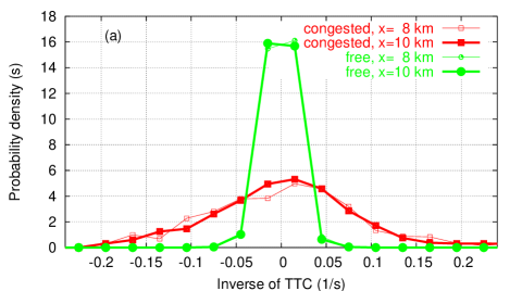
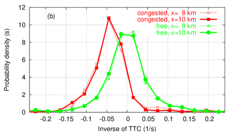
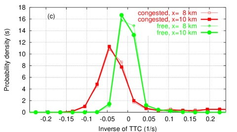
Figure 6: Distribution of the inverse $(v_{\alpha}-v_{\alpha-1})/s_{\alpha}$ of the times-to-collision as calculated from single-vehicle data of virtual detectors for the VDT using (a) the IDM; (b) the OVM; (c) the VDIFF.

Instead of plotting distributions of the TTC directly, we present, in Fig. 6, distributions of the inverse of the TTC, which we denote as ’relative approaching rate’

$$r_{\alpha}=1/\tau\sup{TTC}_{\alpha}.$$ (20)

This has the advantage that the interesting range of small positive and negative values of the TTC is magnified and there is no divergence for the equilibrium state, i.e., $v_{\alpha}=v_{\alpha-1}$. We have obtained the following main results:

• Both in the models and in the empirical data (cf. Fig. 1), the distribution is nearly symmetrical with respect to positive and negative values of $r_{\alpha}$.

• For the OVM and VDIFF, the width of the distribution is nearly the same for free and congested traffic, in agreement with the empirical data, while the variance of the IDM distribution is too small for free traffic.

• For the IDM, the peaks of the distribution are located at $r_{\alpha}=0$ (i.e., equilibrium traffic is the most probable state, in agreement with the data) while the peak for congested traffic is shifted towards negative times-to-collision in the other two models.

The main difference of the IDM with respect to the other models are the order of magnitude of the accelerations. While the IDM acceleration (whose order is given by the parameters $a$ and $b$) did not exceed $\pm 4\mbox{m/s${}^{2}$}\,$, the OVM acceleration varied between $-16\mbox{m/s${}^{2}$}\,$ and $7\,\mbox{m/s${}^{2}$}\,$, and the VDIFF accelerations between $-9\,\mbox{m/s${}^{2}$}\,$ and $5\,\mbox{m/s${}^{2}$}\,$. Since the determination of $r_{\alpha}$ from single-vehicle data via the Eqs. (19) and (20) is only exact for zero accelerations, this is a possible explanation for the asymmetry in the simulation.

V Discussion

In the variance-driven time headway (VDT) model put forward in this paper, the desired safety time headway is a dynamic variable increasing with the local velocity variance. This provides a mechanism for a spontaneous formation and decay of long-lived but non-permanent platoons: If traffic flow is stable, initial velocity differences decrease, leading to decreased values of the local variance and thereby to low values of the desired time headway and a high dynamic road capacity. Because of the conservation of the vehicle number, this automatically leads to platoons and to large gaps in front of the slowest vehicles (’trucks’). For sufficiently high traffic demands the short time gaps may result in unstable traffic flow, leading to higher values of the variance. This, in turn, causes spontaneous braking maneuvers of the drivers which further increase the velocity variance. Finally, this breaks up the whole platoon resulting in a traffic breakdown with a distinct capacity drop.

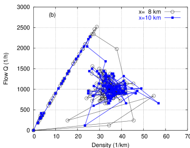
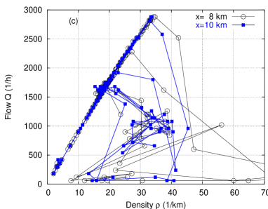
Figure 7: Simulated flow-density data of the VDT applied to the IDM at two ’virtual detectors’ with a sampling interval of $T_{\mathrm{aggr}}=60$ s (a) with fluctuations; (b) without fluctuations; (c) without fluctuations and on-ramp vehicles merging with the speed of the vehicles on the main road rather than half of it as in (a) and (b).

Our intention is to propose a simple model for this variance-driver mechanism. Therefore, we have neglected, e.g., finite reaction times or more elaborated concepts of anticipation which are contained, for example, in the human driver model (HDM) Treiber et al. (2005). Furthermore, we have modeled fluctuations in the simplest possible way.

In the following, we want to discuss our main results in the light of the ’VDT mechanism’:

• The distribution of time headways in free traffic is broad and asymmetric both in the deterministic and stochastic cases, although all vehicles (cars and trucks) have the same time-headway parameter. The reason is that the time headway depends dynamically on the velocity variance. Consequently, even the deterministic driver-vehicle units do not have a unique fundamental diagram.

• The averaged time headway in congested traffic is almost twice of that in free traffic (Figs. 1 and 3), which is related to the higher values of the velocity variation coefficient for congested traffic compared to free traffic.

• Apart from the IDM, the distribution of the relative approaching rates (inverse of the times-to-collision) is nearly independent of whether traffic is free or congested. This is a result of several antagonistic effects: In congested traffic, the velocity correlation $r_{v_{\alpha},v_{\alpha-1}}$ between neighboring vehicles, the variation coefficient $V$, Eq. (2), and the time headway $T$, Eq. (1), are all higher than in free traffic. In the approximate expression for the standard deviation of the relative approaching rate defined in Eq. (20),

  $$\sqrt{\mbox{$\langle r_{\alpha}^{2}\rangle$}}=\frac{V(1-r_{v_{\alpha},v_{\alpha-1}})}{T},$$ (21)

  these three influences essentially cancel out each other for suitable parameter choices.

• On a macroscopic level, the VDT reproduces the wide scattering of data points in the flow-density diagram calculated from one-minute data (Fig. 7), and the capacity drop at the transition from free to congested traffic (Fig. 7(a)).

In presenting our simulation results, we have emulated the available data analogously to real traffic data. For example, we did not use the full information of all vehicle trajectories for plotting the spatiotemporal dynamics of the velocity. Instead, we have restricted ourselves to ’virtual detectors’, as this approach allows a direct comparison with empirical traffic data.

We note that an understanding of the effects of the velocity variance is crucial for devising measures to avoid traffic breakdowns: The VDT feedback mechanism is triggered most likely near sources of sustained velocity variations, for example in the merging, diverging, or weaving zones near freeway intersections, but also the noise term plays a role. To illustrate that, we have introduced a sustained velocity perturbation in all simulations of Sec. IV and in Figs. 7(a) and (b) by letting accelerating ramp vehicles merge with only half the velocity of the vehicles on the main road. In simulations where the ramp vehicles entered with the speed of the vehicles on the main road, we observed a markedly delayed traffic breakdown occurring only after a traffic-flow peak near 3000 vehicles/h instead of 2500 vehicles/h, cf. Fig. 7(c). The subsequent breakdown, however, was more severe showing not only ’synchronized traffic’ but also jammed traffic with nearly vanishing flows. Eliminating the noise term alone had a smaller effect (Fig. 7(b)).

Thus, it is essential to avoid merging and diverging maneuvers at high velocity differences, e.g., by increasing the length of the acceleration lane at on-ramps and off-ramps. Another measure to reduce the velocity variance are speed limits which can be simulated with the VDT as well. Furthermore, since lane changes constitute another source of velocity variance, we expect a strong coupling of lane changes to the longitudinal dynamics by the VDT mechanism. In particular, a multi-lane generalization of the VDT Treiber and Helbing (2002) might yield a fully quantitative explanation of bottleneck effects introduced by weaving zones and off-ramps.

Finally, the distinct increase of the time headways after traffic breakdown opens up vehicle-based options to increase traffic performance and stability by means of adaptive-cruise control (ACC) systems. Such driver-assistance systems, which accelerate and brake automatically depending on the distance to the preceding vehicle and its velocity, are already commercially available for some upper-class vehicles. By a suitable strategy for varying the time headways of ACC systems as a function of the traffic situation, the unfavorable human behavior can be partially compensated for. First simulations of such ACC-systems show promising results Treiber and Helbing (2001).

Acknowledgments: The authors would like to thank for partial support by the Volkswagen AG within the BMBF project INVENT.

References

- (1)
- Neubert et al. (1999) L. Neubert, L. Santen, A. Schadschneider, and M. Schreckenberg, Phys. Rev. E 60, 6480 (1999).
- Tilch and Helbing (2000) B. Tilch and D. Helbing, in Traffic and Granular Flow ’99, edited by D. Helbing, H. Herrmann, M. Schreckenberg, and D. Wolf (Springer, Berlin, 2000), pp. 333–338.
- Kerner and Rehborn (1996) B. Kerner and H. Rehborn, Phys. Rev. E 53, R4275 (1996).
- Nishinari et al. (2003) K. Nishinari, M. Treiber, and D. Helbing, Phys. Rev. E 68, 067101 (2003).
- Helbing (2001) D. Helbing, Review of Modern Physics 73, 1067 (2001).
- Kerner (2004) B. S. Kerner, The Physics of Traffic. Empirical Freeway Pattern Features, Engineering Applications, and Theory, Understanding Complex Systems (Springer, Heidelberg, 2004).
- Knospe et al. (2002) W. Knospe, L. Santen, A. Schadschneider, and M. Schreckenberg, Phys. Rev. E 65, 056133 (2002).
- Treiber et al. (1999) M. Treiber, A. Hennecke, and D. Helbing, Phys. Rev. E 59, 239 (1999).
- Hirst and Graham (1997) S. Hirst and R. Graham, in Ergonomics and Safety of Intelligent Driver Interfaces, edited by Y. Noy (Lawrence Erblaum Associates, New Jersey, 1997).
- Minderhoud and Bovy (2001) M. M. Minderhoud and P. H. L. Bovy, Accident Analysis & Prevention 33, 89 (2001).
- Hall and Agyemang-Duah (1991) F. Hall and K. Agyemang-Duah, Transportation Research Record 1320, 91 (1991).
- Daganzo et al. (1999) C. Daganzo, M. Cassidy, and R. Bertini, Transportation Research B 33, 25 (1999).
- Kerner and Rehborn (1997) B. Kerner and H. Rehborn, Phys. Rev. Lett. 79, 4030 (1997).
- Treiber et al. (2005) M. Treiber, A. Kesting, and D. Helbing, to be published in Physica A (2005), doi:10.1016/j.physa.2005.05.001.
- Lenz et al. (1998) H. Lenz, C. Wagner, and R. Sollacher, European Physical Journal B 7, 331 (1998).
- Treiber and Helbing (2003) M. Treiber and D. Helbing, Phys. Rev. E 68, 046119 (2003).
- (18) M. Treiber and D. Helbing, Explanation of observed features of self-organization in traffic flow, e-print cond-mat/9901239.
- Neubert et al. (2000) L. Neubert, L. Santen, A. Schadschneider, and M. Schreckenberg, in Traffic and Granular Flow ’99, edited by D. Helbing, H. Herrmann, M. Schreckenberg, and D. Wolf (Springer, Berlin, 2000), pp. 307–314.
- Gipps (1981) P. G. Gipps, Transp. Res. B 15, 105 (1981).
- Brackstone and McDonald (1999) M. Brackstone and M. McDonald, Transp. Res. F 2, 181 (1999).
- Nagel and Schreckenberg (1992) K. Nagel and M. Schreckenberg, J. Phys. I France 2, 2221 (1992).
- Knospe et al. (2004) W. Knospe, L. Santen, A. Schadschneider, and M. Schreckenberg, Phys. Rev. E 70, 016115 (2004).
- Kerner and Klenov (2002) B. S. Kerner and S. L. Klenov, J. Phys. A: Math. Gen. 35, L31 (2002).
- Wagner (2004) P. Wagner (2004), cond-mat/0411066.
- Treiber and Helbing (1999) M. Treiber and D. Helbing, J. Phys. A 32, L17 (1999).
- Helbing and Treiber (2002) D. Helbing and M. Treiber, Cooper@tive Tr@nsport@tion Dyn@mics 1, 2.1 (2002), (Internet Journal, www.TrafficForum.org/journal).
- Bando et al. (1995) M. Bando, K. Hasebe, A. Nakayama, A. Shibata, and Y. Sugiyama, Phys. Rev. E 51, 1035 (1995).
- Jiang et al. (2001) R. Jiang, Q. Wu, and Z. Zhu, Phys. Rev. E 64, 017101 (2001).
- Treiber et al. (2000) M. Treiber, A. Hennecke, and D. Helbing, Physical Review E 62, 1805 (2000).
- Chowdhury et al. (2000) D. Chowdhury, L. Santen, and A. Schadschneider, Physics Reports 329, 199 (2000).
- Helbing and Treiber (2003) D. Helbing and M. Treiber (2003), cond-mat/0307219.
- Gardiner (1990) C. Gardiner, Handbook of Stochastic Methods (Springer, N.Y., 1990).
- Treiber and Helbing (2002) M. Treiber and D. Helbing, in ASIM 2002, edited by D. Tavangarian and R. Grützner (Tagungsband 16. Symposium Simulationstechnik, Rostock, 2002), pp. 514–520.
- Treiber and Helbing (2001) M. Treiber and D. Helbing, Automatisierungstechnik 49, 478 (2001).