The Network of Inter-Regional Direct Investment Stocks across Europe

Abstract

We propose a methodological framework to study the dynamics of inter-regional investment flow in Europe from a Complex Networks perspective, an approach with recent proven success in many fields including economics. In this work we study the network of investment stocks in Europe at two different levels: first, we compute the inward-outward investment stocks at the level of firms, based on ownership shares and number of employees; then we estimate the inward-outward investment stock at the level of regions in Europe, by aggregating the ownership network of firms, based on their headquarter location. Despite the intuitive value of this approach for EU policy making in economic development, to our knowledge there are no similar works in the literature yet. In this paper we focus on statistical distributions and scaling laws of activity, investment stock and connectivity degree both at the level of firms and at the level of regions. In particular we find that investment stock of firms is power law distributed with an exponent very close to the one found for firm activity. On the other hand investment stock and activity of regions turn out to be log-normal distributed. At both levels we find scaling laws relating investment to activity and connectivity. In particular, we find that investment stock scales with connectivity in a similar way as has been previously found for stock market data, calling for further investigations on a possible general scaling law holding true in economical networks.

I Introduction

In this work we study the network of investment stocks in Europe at two different levels of graining, a finer and a coarser level. We start by studying the network of investment stocks between individual firms and we then proceed to study the network of investment stocks between European regions. At each level we focus on two specific aspects of such networks: on one hand the statistical distributions of activity, investment stock and connectivity degree. On the other, the scaling relations between such quantities. In this respect this work is related to previous ones in Complex Networks, in economic networks, and also in scaling laws in industrial economics.

Several authors within the Complex Networks scientific community have started to focus today on the geographical aspects of empirical networks like for instance the world wide air traffic network Barrat/Barth/Vesp:05:SpatConstrInAirNet ; Guimera/Mossa/Turtschi/Amaral:05:AirNet .

Closer to economics, some authors have studied the so called World Trade Web (WTW), i.e. the network of import-export trade among countries in the world Garlaschelli/Loffredo:04:WTW ; Serrano/Boguna:03:WTW . Also, statistical properties of ownership networks have been studied so far only in a few works, and in any case with no focus on geographical aspects. To name a few of the works in this area, a study on the firm ownership network of Germany found it to exhibit small world properties Kogut and Walker 1999 . In the US stock markets, power law distribution of connectivity degree and scaling relation between degree and invested volume have been found Garlaschelli/Battiston/al:05:SFTopo . However, it has been observed that network structures may differ from each other in terms of control concentration and still look similar from the point of view of the degree distribution or the investment volume distribution Battiston:04:InnerStructCapitNets .

In the economic literature, some works consider geographical embedding of economic networks. It has been argued that domestic rivalry and geographic industry concentration are especially important in creating dynamic clusters Jakobsen/Onsager:04:HeadOfficeLocation . From a more general perspective, some authors assume the existence of a global world-economy in which, since its inception in the sixteenth century, the periphery is assigned the function of supplying the core with cheap labor and raw materials, while the core has the role of producing manufactured goods, which require capital intensive high technology Wallerstein:74:ModernWorldSystemI .

Statistical distributions in firm demography are well documented: firm size Axtell:01:Science ; Sutton:97 , firm growth Fujiwara/DiGuilmi/Aoyama/Gallegati:03:ParetoZipf , firm debts DelliGatti/DiGuilmi/Gallegati:03 have been studied in several countries and contexts. However, in general, interactions are poorly considered in empirical studies. Firms are not isolated, but rather depend on the interaction with other ones through supply, ownership, partnership relations etc. Such relations should then play a role in the statistical properties observed at a macroscopic scale. Also, there exists an interaction between firms and banks through loans, and it has been found that the distribution of the so called ”bad debts” (debts of firms towards the bank when they go bankrupt) is power-law distributed. Another type of interaction which is not well documented are the investment stocks of firms in other firms. In this paper we find a power law distribution for investment stock with an exponent very close to the one found for firm activity (measured in number of employees, see section II). Such a finding suggests a scaling law between investment and activity that we also investigate and discuss. It is relevant to mention here the relationship between empirically observed macroscopic distributions and possible microscopic processes that may be responsible for them. In literature about the emerging of scaling laws in firm demography, power law distributions are usually obtained as a result of a random multiplicative process affecting the size of each firm. Now, it is known from the works of Kesten in the 70’ies that under some general conditions, a combination of random multiplicative and additive process can give rise to power law distributions Kesten:73:RandomDiff . Even a random multiplicative process with a lower reflecting barrier (representing for example a bankruptcy threshold below which a firm disappears and a new one is created) gives rise to a power law distribution. Instead, a pure random multiplicative process gives rise to a log-normal distribution Sornette:98 . However, in all these processes, interaction between firms is not considered. Among the few works addressing the issue, we mention one in which a firm bankruptcy affects indirectly other firms through the interest rate of the central bank Delli Gatti/al:03:NewApprBusinessFluct . In this paper we start filling such gap by focusing on the distribution and the scaling properties of investments of firms in other firms. Our aim is to contribute to the understanding of how interdependency between firms gives rise to well defined statistical distributions both at the level of firms as at the level of regions.

I.1 Foreign Direct Investments and Inter-Regional Direct Investments

Concerning investment there is a tendency to study investment stocks or flows between countries, referred to as Foreign Direct Investment (FDI), without considering a higher resolution. Contrary to this tendency, in this paper, we focus on investment stocks between regions of Europe, which can be referred to as Inter-Regional Direct Investment (IRDI). In this sense, as discussed later, some concepts will be borrowed from the FDI literature and applied in the IRDI context. The statistical characterization of the network of IRDI stocks in Europe is a first step towards relating investment flow patterns at a global level to local and regional dynamics.

FDI is defined as ”investment that adds to, deducts from or acquires a lasting interest in an enterprise operating in an economy other than that of the investor” the purpose is to have an ”effective voice in the management of the enterprise”, as equivalent to holding 10% or more in the foreign enterprise ONS-UNCTAD:FDI_def . Foreign affiliates are made up of subsidiaries, associates, and branches. Subsidiaries are majority- or wholly-owned by the parent companies. Associates are companies in which the investing firm participates in the management but does not exercise control. Branches are permanent establishments set up by the parent company in which there is no equity share capital apart from that of the parent. For associates and subsidiaries, FDI flows consist of the net sales of shares and loans (including non-cash acquisitions made against equipment, manufacturing rights, etc.) to the parent company plus the parent firm’s share of the affiliate’s reinvested earnings plus total net intra-company loans (short- and long-term) provided by the parent company. For branches, FDI flows consist of the increase in reinvested earnings plus the net increase in funds received from the foreign direct investor. FDI flows with a negative sign (reverse flows) indicate that at least one of the components in the above definition is negative and not offset by positive amounts of the remaining components. However, the magnitude of FDI flow can also be measured as number of jobs created or increased. Contribution to more favorable employment status in the host country is critical when evaluating FDI, especially for countries that are battling high unemployment rates or want to increase the quality of their workforce. When quantifying FDI, ”flow” (function of time) and ”stock” (cross-sectional/cumulative) are measured and headquarter location of the investor plays a critical role Jakobsen/Onsager:04:HeadOfficeLocation .

Due to standard legal, institutional and policy attributes that are common across a given country it indeed makes sense to focus on FDI. However, nowadays firms may perceive some regions in another country as more similar than regions within national borders. This might be revealing that the process of European integration has reduced the national specificities perceived by multinationals and that regions now are competing to attract FDIs more across than within countries. Therefore it is important to gain insight on investment flows at a higher spatial resolution. In this paper we define Inter-Regional Direct Investment (IRDI) flow in analogy to FDI, as the flow between two administratively separated regions irrespective of their countries.

I.2 Relevance of FDI/IRDI for the Global Economy

Just like FDI, the study of IRDI has prominent policy making implications, in particular for governing bodies trying to tackle economic growth and employment creation IFC:Policies . There are certain general factors that consistently determine which countries/regions attract the most investment Borensztein/DeGregorio/Lee:98 . In particular, investors cite the following: market size and growth prospects of the host, wage-adjusted productivity of labor, the availability of infrastructures, reasonable levels of taxation and the overall stability of the tax regime. Recent crises have magnified perceptions of regulatory risks and greater attention is now being focused on the legal framework and the rule of law. Thus the decision process in investment is multi-factorial whereas the success or a higher productivity of the investment holds only when the host country/region has a minimum threshold stock of human capital. Thus, investment contributes to economic growth only when a sufficient absorptive capability of the advanced technologies is available in the host economy Loungani/Razin . Promotional efforts to attract investment have become the focal point of competition among developed and developing countries. This competition is maintained even when countries are pursuing economic integration at another level. And it also extends to the sub-national level, with different regional authorities pursuing their own strategies and assembling their own basket of incentives to attract new investments. While some see countries lowering standards to attract FDI in a ”race to the bottom,” others praise FDI for raising standards and welfare in recipient countries. The targets for these promotional efforts are dominantly the major players of FDI, namely the Transnational Corporations (TNC’s) who on the other end push for newer markets (in the last decades the global trend of privatization has been a very important mean towards this end). Public interest driven policies meanwhile continue to serve as the balancing force, and sustainable development concerns are dealt with accordingly. The EU has attracted over 40% of total world flows of FDI in the 1990s, becoming the largest recipient of multinational activity: multinationals account for a growing share of gross fixed capital formation in Europe (from 6% in 1990 to over 50% in 2000). However, this increasing inflow of FDI in Europe has not been equally distributed across countries and regions Basile/Castellani/Zanfei:03:LocationChoiceMultinat .

Now, while statistics are mostly regarded at the country-to-country scale, investments are actually made in specific regions with geographic features, local administration constraints, and cultural profile. There seem to be a substantial gap to fill in understanding what is the role of region-to-region investment flow in the global economy. For this reason we hereby propose to define the IRDI stock network and we investigate some of its statistical properties as a first stage of a more comprehensive study to be continued in the future. In section II we describe the data set analysed and discuss some methodological issues. In section III we present and discuss the results of our analysis. In section V we draw the conclusions and list some possible extensions of the present work.

II Data Sets and Methods

In this section we first describe the content of the firm database we used for our analysis. We then introduce the quantities we have measured on the data set and include some methodological remarks.

For the firm information we used data collected in December 2004 from the Amadeus database of Bureau Van Dijk. Access to the on-line service of Amadeus is costly and was kindly granted by Prof. Delli Gatti of Università Cattolica di Milano. The database provides firm address, financial profile, number of employees, industrial classification, names of shareholders and board of directors of virtually all firms in Europe.

However data are delivered in files of limited size and we were forced to restrict the download to a selection of the ensemble of firms. We have chosen to select the firms with number of employees larger or equal to 100. Also, a small percentage of around 1% of firms was lost in this selection because the number of employees was not available. The original data set consists of 181.945 firms from 39 European countries uniquely identified by their Bureau Van Dijk identification number (BVDID). For a given firm, shareholders can be individuals/families, governments or other institutions that are not listed as firms. Even when they are firms they may have only indirect ownership through intermediate firms. Moreover, they may have less than 100 employees and therefore location and profile for them is not available in our data set. The set of firms which are involved in ownership links with other firms includes 47.621 firms. We have chosen to restrict our analysis to the direct ownership network of firms with more than 100 employees, implying that we have the financial profile and geographical location of all the firms involved in this set of ownership links. This is the set of data we use for the network analysis and it includes 29.314 firms and 22.174 links.

The selection of a subset of the ownership links induces of course an underestimation of the total hosted investment stock. Still, investigating how investment size among this set of firms is distributed in the network and among geographical regions is a very interesting point to address.

II.1 Defining the Quantities of Interest

For each firm $i$ we consider the following quantities: the activity $a_{i}$ measured as number of employees in the firm, the shares $w_{ij}$ of firm $i$ owned by any other firm $j$, and the headquarter region $R_{i}$ of firm $i$. The number of employees is one of the standard quantities used to measure firm size Axtell:01:Science , and in the following we will measure also investment stocks in terms of number of employees. There are of course other possible measures of investment stocks, based on capital rather than on human resources, but from the point of view of labour market and economic impact at a local scale, it is relevant to have an estimate of how many employees of a firm or a region depend on the investment coming from outside.

Figure 1: Diagram illustrating how the (right) region network $G_{R}$ is built up from the (left) firm network $G_{F}$.

Shares are usually defined as a percentage, but it is more convenient to define $w_{ij}$ as a fraction of ownership and, therefore, as a real number in $[0,1]$. Not all shares are necessarily held by entities external to the firm. Moreover some entities are not firms and we only look at shares held by firms, as discussed above. Therefore it holds:

$$\sum_{j\neq i}w_{ij}\leq 1$$ (1)

If we take the number of employees as a measure of activity of a firm, it is natural to compute the quantity $s_{ij}$:

$$s_{ij}=w_{ij}a_{i}$$ (2)

that represents the investment stock of firm $i$ held by firm $j$.

We can define the firm network as a graph $G_{F}=(V_{F},E_{F})$ Figure 1(left) where $V_{F}$ is a set of nodes representing firms and $E_{F}$ is a set of directed edges between nodes. An edge $(i,j)$ represents the fact that firm $j$ owns shares of firm $i$. The order of the pair in this notation is natural for the layout of most databases of firms and we adopt it. However, keep in mind, that ownership and investment have opposite directions. In fact, it is more natural to define in-degree and out-degree of connectivity with respect to investments rather than to ownership. We define as in-degree $k_{in}$ of a firm the number of firms investing in $i$ (holding shares of $i$). Similarly we define as out-degree $k_{out}$ of a firm the number of outside firms in which firm $i$ invests. The connectivity degree or simply degree $k$ of a node is the number of edges entering or departing from that node.

We can associate to each edge $(i,j)$ the normalized weight $w_{ij}$, representing the amount of shares that firms $j$ owns in $i$. But we can also associate the absolute weight $s_{ij}$. We then define the inward investment stock $a_{i}^{in}$ of firm $i$ , as the total stock invested in firm $i$ by other firms and outward investment stock $a_{i}^{out}$, as the total stock invested by firm $i$ in other firms:

$$a_{i}^{in}=\sum_{j}s_{ij}\hskip 28.45274pta_{i}^{out}=\sum_{k}s_{ki}$$ (3)

We can now define analogous quantities aggregated by region. The activity of region $m$ is defined as the sum of the activity of the firms with headquarter in that region.

$$A_{m}=\sum_{i\in m}a_{i}$$ (4)

In other words, $A_{m}$ is the total number of workers employed by firms of that region. Keep in mind that we analyse only a subset of all firms and that therefore, the activity of a region can be much smaller than the number of individuals employed in that region. The sum of the investments made by firms of region $n$ in firms in region $m$ is defined as:

$$S_{mn}=\sum_{i\in m,j\in n}s_{ij}$$ (5)

It can be seen both as the outward investment stock of region $n$ in region $m$ or as the hosted investment stock in region $m$ coming from region $n$

It is very natural at this point to define the region network as a graph $G_{R}=(V_{R},E_{R})$ where nodes represent regions and a directed edge $(m,n)$ from region $m$ to region $n$ represents the fact that some firms of region $n$ own shares in some firms of region m. The diagram in figure 1 illustrates the procedure of building the network of regions. Small circles represent firms with their associated values of activity. Edges represent ownership relations. Larger circles represent regions in which firms have their headquarters. The edges in firm network among all firms in regions $m$ and $n$ sum up to form an edge between m and $n$ in the region network. We associate to the edge $(m,n)$ the absolute weight $S_{mn}$. The degree is defined as for the firm region and in particular in-degree and out-degree are defined with respect to investments.

The sum of the investments made in firms of a region by firms of any other region will be called inward investment stock of region m (eq.6). In the following we will refer to this quantity also as hosted investment stock. Similarly, the sum of the investments made by the firms of a region in firms of other regions will be called outward investment stock of region m (eq.6).

$$A_{m}^{in}=\sum_{n}S_{mn}\hskip 28.45274ptA_{m}^{out}=\sum_{n}S_{nm}$$ (6)

Both definitions are chosen in analogy with the terms used in the literature about Foreign Direct Investments. But instead of looking at investments between different countries, we increase the spatial resolution to the level of regions.

As only the few most important shareholders of each firm are usually listed in the database, the in-degree of firms is a bias quantity with little meaning for our purposes. However, when aggregating by region, the in-degree of a region represents the number of other regions in which the top shareholders of firms in the focal region have their headquarters. This quantity is not limited a priori and as such it makes sense to study its distribution.

II.2 Measuring the Quantities of Interest

Our perspective in this work is to try and relate the microscopic and macroscopic aspects of the network of investments between firms and between regions. We want to look at statistical distributions and not at single or average values, the aim being to try and understand what is the individual tendency that builds up the macroscopic properties. Therefore we will focus on the probability distributions of the quantities defined above.

In order to study the probability distribution (pdf) of a variable $x$ it is useful to plot its cumulative distribution function (cdf) defined as

$$P_{C}(\hat{x})=\int_{x\geq\hat{x}}p(x)dx$$ (7)

where $x\rightarrow p(x)$ is the probability distribution function. In words, the cdf gives the fraction of a randomly chosen sample of the variable $x$ that lies above the value $\hat{x}$. A simple way of constructing $P(x)$ is the following. Consider the vector $x$ of $N$ real numbers. We rank $x$ in ascending order. Clearly, now all values are larger or equal to the first data point. So the probability distribution starts from 1 and decreases. The k-th component of the vector $x$ has ascending rank $k$ and there are $N-k$ values larger or equal to $x(k)$. The fraction of data larger or equal to $x(k)$ is $N-k/N$. We therefore simply plot the pair $(x(k),N-k/N)$ for all $k$. If some values of $x$ are repeated and in particular if $x$ is a discrete variable, then the plot will display ’stairs’. In this case it is preferable to count the fraction $P$ of data that are larger or equal to each value $x$ and then to plot $P$ versus $x$.

If the distribution of the variable $x$ is a power law with exponent $-\gamma$, then its cumulative distribution is still a power law with exponent $-\gamma+1$. In $\log-\log$ scale they appears as straight lines with different slope:

$$p(x)=c_{1}x^{-\gamma}$$ (8)

$$P(x)=c_{2}x^{-\gamma+1}$$ (9)

where $c_{1},c_{2}$ are normalization factors. If instead the distribution of the variable $x$ is log normal with coefficients $\mu$ and $\sigma$ (eq. 10), then it appears as a quadratic curve in $\log-\log$ scale.

$$p(x)=\frac{1}{x\sqrt{2\pi\sigma^{2}}}exp(-\frac{(\log x-\mu)^{2}}{2\sigma^{2}}$$ (10)

$$\log(p(x))\sim-\log(x)-\frac{(\log x-\mu)^{2}}{2\sigma^{2}}$$ (11)

However, its cumulative distribution does not have an analytical expression.

It is usually more accurate and safe to estimate the exponent from the cdf rather than from the pdf, because of the fluctuations in the frequency of high values of $x$. This is usually done by fitting the cdf in $\log-\log$ scale with a line and computing the slope. However, it has been recently remarked that this method introduces a systematic bias Goldstein/Morris/Yen:04 . An alternative method that doesn’t make use of a graphic fit is described in Newman:05:PLReview . The formula for the exponent is

$$\gamma=1+N\left[\sum_{i}\log\frac{x_{i}}{x_{\mathrm{min}}}\right]^{-1}$$ (12)

where $x_{\mathrm{min}}$ is the lower limit of the range of data following the power law. Confidence intervals for $\gamma$ can be computed with the standard bootstrap technique.

When a relation holds between two variables, then their respective probability distributions are also related through the equation:

$$p(y)=p(f(x))=p(x)\frac{df}{dx}$$ (13)

An important consequence is that if, $x$ is power law distributed and $y$ scales as a power law of $x$, then $y$ is also power law distributed, and a relation holds for all the exponents involved (power law distributions are closed with respect to the operation of power law rescaling). If $x$ is log normal distributed, and $y$ scales as a power law of $x$, then the distribution of $y$ converges to a log normal function for large $y$. This observation implies that, if two variables are both power law distributed, and we suspect that a relation might hold between them, such relation could be a power law scaling, therefore we have to be careful while checking for possible correlations.

In fact, in the study of the correlation between quantities, related to firms and regions, that span several order of magnitude and have to be studied in $\log-\log$ scale, we proceed as follows. Consider the variables $(X,Y)$ for instance. We compute the $\log{10}$ of both variables and produce a scatter plot of $(\tilde{X},\tilde{Y})=(\log{10}X,\log{10}Y)$. We then divide the X axes in $k$ bins of equal size. For each bin centered in the value $x_{i}$, we compute the mean $y_{i}$ and the standard deviation $\sigma_{y_{i}}$ of the values of $Y$ for which the corresponding abcissa falls in the bin $k$. We obtain a new set of data points $(x,y)$ that allows to better display the trend of the original data $(X,Y)$. A linear fit is then performed on the $(x,y)$ data points, and values of slope, intercept and correlation coefficient are computed. We remind that a linear relationship between $x$ and $y$ implies taking the exponential, a power law relationship between the original variables:

$$\tilde{Y}=m\cdot\tilde{X}+q$$ (14)

$$\log{10}(Y)=m\cdot\log{10}(X)+q$$ (15)

$$Y=C\cdot X^{m}$$ (16)

where $C=10^{q}$. Of course, while the operation of binning and averaging over bins is a standard procedure one should be careful in this case, as such operation does not commute with the operation of taking the exponential. However, we are not aware of any documented bias introduced by this procedure and if the fit is reasonably good we conclude that $Y$ is scaling as a power law of $X$ and we take $m$ as the exponent of the scaling law.

III Analysis at the level of firms

We first report the cumulative frequency distribution of activity and investment stock of firms. We also investigate how investment stock scale with firm activity and with firm connectivity degree. We then report the analogous results for regions where activity, investment stock and connectivity degree of regions are defined as in section II.1. Similarly, we investigate how investment stock scale with region activity and region connectivity degree.

III.1 Firms. Distributions of activity,investment and connectivity degree

In figure 2 we report the cumulative distribution (cdf) of activity and investment stock of firms computed from our data set. The onset at the value 100 for the activity is simply due to the restriction of the data set to firms with more than 100 employees. Investment stock can of course take smaller values as it is measured as a fraction of the number of employees per firm. The cumulative distributions display a linear decay over 3 decades or more. However some ’bumps’ deviating from linearity are visible. The curves can either be fitted with $\log$ normal distributions with very large standard deviation or can be reasonably fitted with a power law. In both cases the meaning is the same: the probability of finding large firms is decreasing approximately as the exponent of the power law fitting the curve. Computing the exponent from the linear fit is known to introduce bias Goldstein/Morris/Yen:04 , hence following a known procedure Newman:05:PLReview the values of the exponents and confidence intervals were computed as described in II. The values of the exponents and their confidence interval are reported in table 1.

Table 1: Firms. Power law fit values for Cumulative Distributions.

Data	$\gamma$	$\sigma_{\gamma}$
$a$	1.7829	0.0038
$a^{in}$	1.9307	0.0064
$a^{out}$	1.7684	0.0061
$a^{in+out}$	1.8480	0.0047
$k^{out}$	3.849	0.044

Our finding concerning the activity is in line with what is generally known in the literature for firm size distributions of many countries and historical epochs. It implies that firm activity is very heterogeneous and that roughly speaking, very large values and very small values of activity are much more frequent that in normal distributions. We remind the reader that the data set analysed includes only firms involved in an ownership relationship in Europe and not all firms indiscriminately. However, the value of exponent $\gamma$ is not far from results obatined in previous studies. For instance Axtell reports 2.056 for the US firm activity distribution Axtell:01:Science . Fujiwara et al. report 1.995 for UK based on data from Amadeus Database Fujiwara/DiGuilmi/Aoyama/Gallegati:03:ParetoZipf . On the other hand, the fact that investment stock distribution is also a power law is to our knowledge a novel result. In particular, the values of the exponent $\gamma$ for activity and outward investment stock are very close.

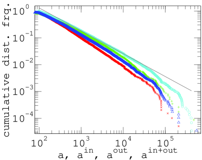
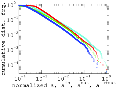
Figure 2: Firms. Cumulative distribution of: (left) activity $a$ (o); hosted investment stock $a^{in}$ ($\times$); outward investment stock $a^{out}$ (+); total investment stock $a^{in+out}$ ($\Delta$) and (right) normalized values with respect to the maximum value

This finding might suggest that a scaling relation holds between the two variables (as discussed in section II.2). However, this hypothesis had not been empirically verified so far in the literature and we don’t know a priori to what extent it holds. We will then investigate its validity in the next section.

As is usual in the study of networks, we report the cumulative distribution functions (cdf) of the degree of connectivity of firms (figure 3 ). We distinguish between (total) degree, in-degree and out-degree as defined in II.1. The distributions span a short range of less than two decades. The out-degree display a linear decay in $\log-\log$ scale that can be fitted by a power law with exponent 3.85, which is a little larger than the typical values observed in many empirical complex networks (typically in the range [1.8 3]). The result implies that the number of connections between firms is moderately heterogeneous and decreases slower than exponentially. The curve for the in-degree instead is not meaningful as mentioned in section II.2 and simply shows how many records of shareholders are available per firm. The linear fit was performed just for sake of completeness.

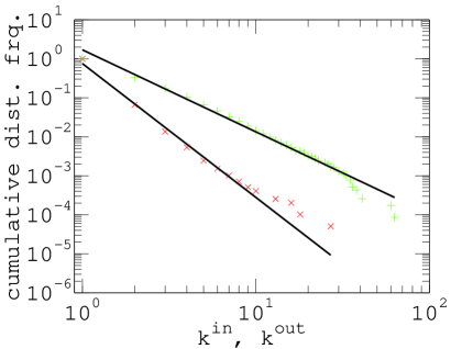
Figure 3: Firms. Cumulative distribution of connectivity degree. In-degree ($\times$) , out-degree (+)

However, it is important to remark that the connectivity out-degree represents the number of ownership relations in which the firm is involved, regardless of the size of shares involved in each relation. Because the degree doesn’t take into account the size of the shares, a large out-degree doesn’t mean that a firms really controls a lot of other firms. Alternative quantities are needed to characterize the ownership concentration such as those introduced in Battiston:04:InnerStructCapitNets and they will be applied to the present data set in a future study.

III.2 Firms. Correlations among activity, investment and connectivity degree

In order to understand why investment of firms are power law distributed and why distributions of outward investment and activity have exponents very close to each other we investigate the correlations between activity, investment and connectivity out-degree. The plots in figures 4 - 5 are produced by taking the $\log 10$ of the quantities and binning the data on the x axes as described in section II.2.

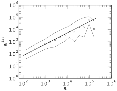
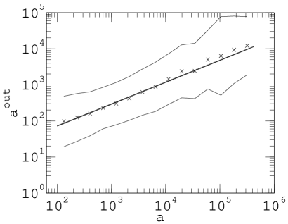
Figure 4: Firms. Plot of (left) hosted invested stock $a^{in}$ and (right) outward invested stock $a^{out}$ of firms versus their activity $a$ in $\log-\log$ scale. Data are binned. Mean $\pm$ standard deviation of the values in each bin are plotted as the continuous lines.

Table 2 reports the value of slope and correlation coefficients for the linear fit of the binned data. The correlation coefficients are all quite close to 1 so, with the caveat mentioned in section II.2, we conclude that the data indicate the existence of scaling laws between investment and activity and between out-degree and activity.

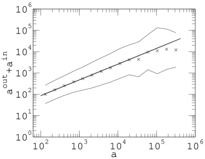
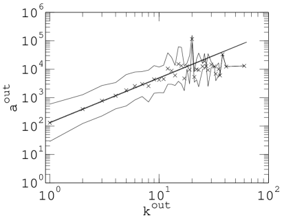
Figure 5: Firms. (left) Plot of total invested stock $a^{in+out}$ of firms versus their activity $a$. (right) Plot of connectivity out-degree $k^{out}$ of firms versus their hosted investment stock $a^{out}$ in $\log-\log$ scale. Plot Data are binned. Mean $\pm$ standard deviation of the values in each bin are plotted as continuous lines.

Table 2: Firms. Scaling of investments versus activity. Coefficients of linear fit and correlation coefficients.

Yaxis	$m$	$q$	corr.coef.
$a^{in}$	0.925	0.026	0.974
$a^{out}$	0.607	0.644	0.997
$a^{in+out}$	0.739	0.460	0.992

We notice that the exponent $0.925$ for the scaling of hosted investment versus activity is smaller than, but still close to 1. This means that firms tend to host investment in amount almost just proportional to their activity. This is not surprising if we consider that all firms in the data set analysed, are owned to some extent by some other firm in the data set and in many cases the share is large and close to 1. A deeper understanding would require an investigation of the statistics of the ownership concentration and will be carried out in a future work. On the other hand the exponent $0.61$ for the scaling of outward investment versus activity implies that although more active firms tend to invest more, the investment increases less than linearly as a function of the activity (sub-linear increase). This means that very large and active firms invest less, in proportion, with respect to smaller ones. Such a finding becomes quite important if an institution in charge of attracting investments from firms is trying to estimate the expected investment of firms based on their activity.

Finally, the exponent $1.57$ for the scaling of activity versus out-degree is quite interesting. It implies that the larger the firm the larger the number of investments but the increase is sub-linear. Interestingly, the value of the exponent is not far from the values found for the scaling law between invested volume and degree in some stock markets: 1.1 for Nasdaq, 1.43 for NYSE, 1.59 for MIB Garlaschelli/Battiston/al:05:SFTopo . In that case the invested volume is exactly the analogous quantity to the outward investment. Moreover, the scaling law resembles the one observed inthe context of air traffic networks for a quantity analogous to the outward investment which has been recently introduced as node strength Barrat/Barth/Vesp:05:SpatConstrInAirNet . In that case the exponent found is $1.7$. These findings might support the idea that a universal scaling law for node strength holds in complex networks where the weight plays a crucial role. In a future work we will investigate possible network formation models leading to the emergence of such scaling law in economic networks.

Table 3: Firms. Scaling of investments versus connectivity degree. Coefficients of linear fit and correlation coefficients

Yaxis	$m$	$q$	corr.coef.
$a^{out}$	1.574	2.120	0.855

IV Analysis at the Level of Regions

IV.1 Regions. Distributions of activity, investment and connectivity degree

In figure 6 (left) we report the cumulative distribution of activity $A$ and inward/outward/total investment stock $A^{in}$, $A^{out}$, $A^{in+out}$ for regions. These quantities were computed from the data set as described in section II.1. As done for the case of firms, in order to check to what extent they overlap we also normalized such quantities and we report their cumulative distribution in figure 6 (right) . As it can be seen, the overlap is only partial. This may suggest that a non linear scaling holds between the variables and this hypothesis will be investigated in the next section.

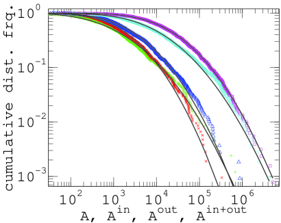
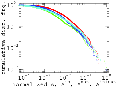
Figure 6: Regions. Cumulative distribution of: (left) activity $A$ (for all firm profiles) ($\square$); activity $A$ (o); hosted investment stock $A^{in}$ ($\times$); outward investment stock $A^{out}$ (+); total investment stock $A^{in+out}$ ($\Delta$) and (right) the same quantities normalized with respect to the maximum value. Zoom.

It must be remarked that the way regions are defined within a country surely depends on the country’s administrative system. To give an example, the regions provided in the data set are at the level of ’provincia’ for Italy and ’department’ for France which have comparable surface on average.

Table 4: Regions. Log normal fit values for Cumulative Distributions.

Data	$\mu$	$\Delta\mu$	$\sigma$	$\Delta\sigma$
$A$	9.06	0.12	1.97	0.08
$A_{alldataset}$	9.79	0.10	1.82	0.07
$A^{in}$	7.28	0.10	1.64	0.07
$A^{out}$	6.89	0.14	2.02	0.10
$A^{in+out}$	7.69	0.10	1.76	0.07
$K$	1.98	0.07	1.18	0.05
$K^{in}$	1.50	0.06	1.00	0.04
$K^{out}$	1.52	0.08	1.16	0.06

Table 5: Regions. Power law fit values for Cumulative Distributions.

Data	$\gamma$	$\sigma_{\gamma}$
$A$	2.29	0.14
$A_{alldataset}$	2.23	0.09
$A^{in}$	2.58	0.19
$A^{out}$	2.40	0.20
$A^{in+out}$	2.21	0.11
$K$	2.53	0.09
$K^{in}$	3.00	0.15
$K^{out}$	2.40	0.10

Differently from the case of the firms, the distributions do not display a linear decay in $\log-\log$ scale but rather a quadratic one which we tried to fit with log-normal distributions. The fit with log normal is quite good although a discrepancy can be observed in the right tail. On the other hand, only the very last portion of the distribution could be fitted with a power law. Values for the coefficients of the log normal fit are given in table 4. Just for sake of comparison we also report the exponent of the power law fit of the rightmost tail (table 5)

At a first sight the finding that the distributions above are log normal is puzzling, as one may expect that region activity and investment stocks also scale with a power law. However, the following remark is relevant at this point. Cities ranges from small villages of few inhabitants to metropolis of 10-20 millions. Firms also range from one-person enterprises to multinationals with few hundreds thousands employees. On the other hand, while the position of the boundaries of a region surely is the result of the historical process, the surface and the amount of population within a region is probably limited by administration tasks constraints, in the sense that if the administrative load becomes too heavy, the region is split into two. For instance within a same country there are no regions which are orders of magnitude larger in surface than other regions. On the other hand, it is known that activity of countries measured by Gross Domestic Product is power law distributed with exponent 1 Garlaschelli/Loffredo:04:WTW . So it appears that regions are clearly less heterogeneous with respect to firms and countries. However before trying to draw some implications for economic development policies, it would be interesting to normalize the activity of the regions by the regions surface and/or active population. Unfortunately these data were not available during this work.

In figure 7 we report the cdf of the connectivity degree for regions. All curves are clearly not power laws and we tried to fit them with log-normal functions. Values of coefficients are reported in table 4. The curve for the in-degree is systematically above the one for the out-degree. Given the fact that the pdf is the derivative of the cdf, the plot implies that in the range [1 50] the in-degree is typically smaller than the out-degree while above 50 the opposite holds. We don’t have an explanation for this finding. On the other hand we remind that as in the case of firms, the number of connections is not necessarily meaningful. In fact this is exactly why we have introduced the inward and outward investment stock.

Figure 7: Network of Regions. Cumulative distribution of connectivity degree. In-degree ($\times$) , out-degree (+), total degree ($\Delta$)

IV.2 Regions. Activity, investment and connectivity degree: correlations

In order to understand why investment of regions are log normal distributed and why distributions of inward/outward investment and activity display a partial overlap after normalization (see section II.2), we investigate the correlations between activity, investment and connectivity in/out-degree of regions. With the same procedure used for the case of firms (see section III.2), we produced the plots in figures 8-9 (see section II.2.

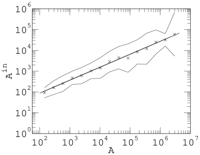
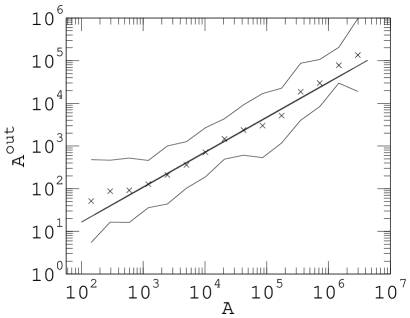
Figure 8: Regions. Plot of (left) hosted invested stock $A^{in}$ and (right) outward invested stock $A^{out}$ of regions versus their activity $A$ in $\log-\log$ scale. Data are binned. Mean $\pm$ standard deviation of the values in each bin are plotted as the continuous lines.

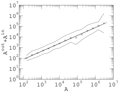
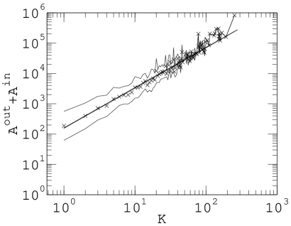
Figure 9: Regions. Plot of (left) total invested stock $A^{in+out}$ of regions versus their activity $A$. (right) Plot of total connectivity degree $k^{tot}$ of regions versus their hosted investment stock $A^{in+out}$. $\log-\log$ scale. Data are binned. Mean $\pm$ standard deviation of the values in each bin are plotted as the continuous lines.

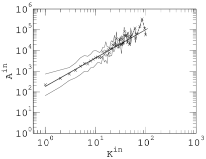
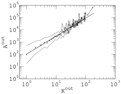
Figure 10: Regions. Plot of connectivity (left) in-degree $k^{in}$ and (right) out-degree of regions versus their hosted investment stock $A^{in}$ and outward investment stock $A^{out}$ respectively in $\log-\log$ scale. Data are binned. Mean $\pm$ standard deviation of the values in each bin are plotted as the continuous lines.

Tables 6,7 report the values of slope and correlation coefficients for the linear fit of the binned data. Again the correlation coefficients are all quite close to 1 so, with the caveat mentioned in section II.2, we conclude that the data indicate the existence of scaling laws in the network of regions between investment and activity and between connectivity degree and activity.

Table 6: Scaling of investments versus activity for regions. Coefficients of linear fit and correlation coefficients.

Yaxis	$m$	$q$	corr.coef.
$A^{in}$	0.623	0.697	0.997
$A^{out}$	0.819	-0.420	0.990
$A^{in+out}$	0.748	0.401	0.998

Table 7: Scaling of investments versus connectivity degree for regions. Coefficients of linear fit and correlation coefficients.

Yaxis	$m$	$q$	corr.coef.
$A^{in}$	1.467	2.022	0.965
$A^{out}$	1.370	2.268	0.965
$A^{in+out}$	1.326	2.201	0.979

We notice that the exponents $0.62$ and $0.82$ for the scaling of hosted investment versus activity and outward investment versus activity respectively are smaller than 1.

As seen at the firm level, it follows that although more active regions tend to make and host more investment, the investment increases less than linearly as a function of the activity (sub-linear increase). This means that very active regions invest, in proportion, less than smaller regions. However, the increase of outward investment with activity is stronger for regions ($m=0.82$) than for firms ($m=0.61$ see table 2). This is an interesting result that we will address in the future.

The amount of investment made or received by regions in relation with their activity is relevant to institutions in charge of fostering development of regions. Although this findings cannot provide detailed prediction they could help develop multi-agent based models trying to reproduced the observed features with the aim of designing possible incentive strategies.

Finally, the exponents for the scaling of activity versus in/out-degree are again not far from the values found for the scaling law in other works such as: between invested volume and degree in stock markets and for the scaling law of node strength versus degree in air traffic networks.

V Conclusions

In this paper we propose a simple but novel procedure to build the network of inter-regional investment, based on the number of employees of firms in each region and their network of ownership. In this network representation, the connectivity in-degree of a region is the number of other regions from which firms invest in the focal region, while the out-degree is the number of regions in which firms of the focal region invest. The sum of the weights over the incoming links represents the hosted investment stock of a region in terms of employees. The sum over the outgoing links represents the outward investment stock of a region in terms of employees.

We study the statistical properties of investment stock networks at the level of firms and at the level of regions. Our first result is that investment stock of firms is power law distributed and that, in particular, the exponent of outward investment is very close to the one of firm activity. As it is well known, this fact may result from a power law scaling relation between activity and outward investment. This is neither obvious nor documented in the literature, so it has to be checked empirically. At a first sight, activity and investment are quite scattered and span a few orders of magnitude. However, by taking the logarithm of the values of activity and investments, and binning the data, we indeed find that investment scales as a power of the activity. Moreover, power law scaling relations also hold between investment stock and connectivity degree.

On the other hand, in the case of regions, we find log normal distributions for activity, investments and degree. Now, it can be argued that this result might simply be related to the distribution of population size across regions (unfortunately we do not have data to test this hypothesis at the moment). Even so, it is a remarkable fact that such probability distributions for the regions clearly differ both from those of firms as from those of countries in the world. The impact of this fact on the design of global policies to foster investments and economic development should be investigated.

Again, the fact that similar distributions emerge for activity, investment and connectivity degree of regions suggests that some relation should hold among them. In particular, we find that investment of firms scales as a power of the degree with exponent 1.57 (out-degree), while for regions it scales with exponents 1.37 and 1.47 (in-degree and out degree respectively). Interestingly, previous studies on different data set have investigated the scaling law of two quantities (invested volume and node strength) strictly analogous to the investment stock and found exponent values between 1.1 and 1.7 Barrat/Barth/Vesp:05:SpatConstrInAirNet ; Garlaschelli/Battiston/al:05:SFTopo . The existence of scaling laws relating investment, activity and connectivity both in firms and regions is an interesting and novel result relevant to the fields of complex networks, industrial economics and geography.

On the other hand, such scaling laws should be of interest for policy making. For instance we find that very active regions invest less, in proportion, with respect to smaller ones. The same holds for firms, although the coefficient governing the relation between investment and activity are different. This kind of result allows to make some statistical predictions about the investments that regions will receive or make, based on their activity and connectivity. The present work is a first step towards understanding the relation between the local dynamics of investment flows and the macro-economical facts emerging at a global level. One can ask for example whether such a distribution of investments is desirable with respect to some societal goals that might be at stake at the country or at the EU level. If it is not, one can investigate if introducing some incentive policies, the distribution can be improved with respect to the goals. In this sense, the findings reported here should stimulate the investigation of models for managing the development of regions and the optimal allocation of resources. Overall, we believe that these results open the way for further studies with potential long run implications in policy making at the level of EU investment promotion, support to underdeveloped EU regions and optimization of investment flow.

VI Acknowledgments

This manuscript greatly benefited from Prof. Frank Schweitzer’s comments. We also thank Prof. Domenico Delli Gatti of Università Cattolica di Milano for granting us access to Amadeus database. S.B. acknowledges the support of CNRS during the phase of data collection and the initial stage of this work. S.B. and J.R. acknowledge the support of the European project MMCOMNET (IST contract n. 12999) and the EXYSTENCE Thematic Institute CHIEF (held at Univ. Politecnica delle Marche, Ancona, IT, May 2-21 2005) where this collaboration has started.

References

- (1)
- (2) Axtell, R.L., Zipf Distribution of U.S. Firm Sizes, Science 293 (2001) 1818.
- (3) Barrat, A., Barthélemy, M., Vespignani, A., The effects of spatial constraints on the evolution of weighted complex networks”, arXiv:physics/0504029 v1 4 Apr 2005
- (4) Basile, R., Castellani, D., Zanfei, A., Location choices of multinational firms in Europe: the role of national boundaries and EU policy, Quaderni di economia, matematica e statistica , n. 76, June 2003, (http://www.fscpo.unict.it/pdf/Castellani
- (5) Battiston, S., Inner structure of capital control networks, Volume 338, Issues 1-2, 1 July 2004, Pages 107-112
- (6) Borensztein, E., De Gregorio, J., Lee, J.W., ”How does foreign direct investment affect economic growth?, Journal of International Economics 45 (1998) 115-135
- (7) Fujiwara, Y., Di Guilmi, C., Aoyama, H., Gallegati, M., Souma, W., Do Pareto-Zipf and Gibrat laws hold true? An analysis with European Firms, arXiv:cond-mat/0310061 v2 27 Nov 2003
- (8) Garlaschelli, D., Loffredo, M.I., Fitness-dependent topological properties of the World Trade Web, Phys. Rev. Lett. 93, 188701 (2004), arXiv:cond-mat/0403051
- (9) Garlaschelli, D., Battiston, S., Castri, M., Servedio, V.D.P., Caldarelli, G., The scale free topology of market investments, 2005, Physica A, Volume 350, 2-4, 491-499
- (10) Gaffeo, E., Gallegati, M., Palestrini, A., Physica A 324 (2003) 117.
- (11) Delli Gatti, D., Di Guilmi, C. and Gallegati, M., On the Empirics of ”Bad Debt”, mimeo, Universit Politecnica delle Marche (2003).
- (12) Delli Gatti, D., Di Guilmi, C., Gaffeo, E., Giulioni, G., Gallegati, M., Palestrini, A., A new approach to business fluctuations: heterogeneous interacting agents, scaling laws and financial fragility, to appear on Journal of Economic Behaviour and Organisation, http://arxiv.org/abs/cond-mat/0312096
- (13) Goldstein, M.L., Morris, S.A., and Yen G.G., Problems with Fitting to the Power-Law Distribution, to appear on EPJ, arXiv:cond-mat/0402322 v3 13 Aug 2004
- (14) Guimerà R., Mossa S., Turtschi A., Amaral L.A.N., The world-wide air transportation network: Anomalous centrality, community structure, and cities’ global roles”, Proc. Nat. Acad. Sci. USA 102, 7794-7799 (2005)
- (15) Kesten, H., Random di erence equations and renewal theory for products of random matrixes. Acta Math., 131, 207-248,(1973)
- (16) Kogut, B. and Walker, G., The Small World of Germany and the Durability of National Ownership Networks, American Sociological Review, 66(3): 317-35, 2001.
- (17) Jakobsen, S.E. and Onsager, K., Head office location Agglomeration, clusters or flow nodes? Urban Studies, August, 2005 Volume 42:9
- (18) Loungani, P. and Razin, A., ”How Beneficial Is Foreign Direct Investment for Developing Countries?” Finance and Development (IMF) June 2001, Volume 38, Number 2
- (19) Newman, M. E. J., Power laws, Pareto distributions and Zipf s law, arXiv:cond-mat/0412004 v2 9 Jan 2005
- (20) Serrano, M.A. and Boguñá, M., Topology of the World Trade Web, Physical Review E 68, 015101 (2003), arXiv:cond-mat/0301015
- (21) Sornette, D., Multiplicative processes and power laws, Phys. Rev. E 57 N4, 4811-4813 (1998)
- (22) Sutton, J., J. Econ. Lit. 35 (1997) 40.
- (23) Wallerstein, I., The Modern World System I. Capitalist Agriculture and the Origins of the European World -Economy in the Sixteenth Century, New York, Academic Press, 1974
- (24) Office for National Statistics (ONS), UK - FDI Profile UNCTAD
- (25) Policies to Attract Foreign Direct Investment, World Bank/IFC. (Web site: Papers and Links - Privatization, Infrastructure & Business Environment)