A selected history of expectation bias in physics

Abstract

The beliefs of physicists can bias their results towards their expectations in a number of ways. We survey a variety of historical cases of expectation bias in observations, experiments and calculations.

It is a capital mistake to theorise before one has data. Insensibly one begins to twist facts to suit theories, instead of theories to suit facts.

Sherlock Holmes Holmes

But are we sure of our observational facts? Scientific men are rather fond of saying pontifically that one ought to be quite sure of one’s observational facts before embarking on theory. Fortunately those who give this advice do not practice what they preach. Observation and theory get on best when they are mixed together, both helping one another in the pursuit of truth. It is a good rule to not put overmuch confidence in a theory until it has been confirmed by observation. I hope I shall not shock the experimental physicists too much if I add that it is also a good rule not to put overmuch confidence in the observational results that are put forward until they have been confirmed by theory.

Sir Arthur S. Eddington Eddington

I Introduction

Under an idealized view of science, the theoretical beliefs of experimenters should have no effect on what results are obtained. Theoretical beliefs can influence what experiments are done, and how they are interpreted and recieved, but the actual results are facts determined purely by nature. But in practice, one can worry that even honest and careful experimenters might still somehow transfer their biases to their end results.

Sherlock Holmes warns against this by forbidding any theorizing in advance of the experiment. But it is difficult to see how this is possible, let along desirable. And when we remember that Sir Arthur Conan Doyle, the author of Sherlock Holmes, uncritically accepted, and indeed actively promoted, the “data” that fairies had been seen and photographed in Cottingley, England fairies , we begin to think that perhaps not all “experimental facts” should be accepted and treated equally. Eddington’s characterization of the complex interplay between theory and experiment seems to come closer to the truth. Perhaps the facts from experiments and observations are not always simple “facts,” to be accepted at face value.

Expectation bias is well-known, and widely discussed in the “softer” sciences, that study humans, such as psychology and medicine. But what role does it play in “hard” sciences, such as physics? The impression one gets from the history in physics textbooks is that it plays virtually no role, but this may be misleading. Because textbooks have as their primary goal to teach physics, extended discussions of how this physics was arrived at can seem like pointless and potentially confusing diversions; the emphasis is on how careful and correct reasoning leads to correct results, even if that reasoning is retrospective, and ahistorical. Convoluted reasoning that was actually followed is replaced with the clearer reasoning that “should” have been followed. Many readers will doubtlessly be surprised to discover that Planck was not led to quantization in an attempt to fix an “ultraviolet catastrophe” discovered by Rayleigh History.Brush ; History.Whitaker , that Rømer never calculated a value for the speed of light Romer , and that Einstein was not primarily motivated by the Michelson-Morley experiment in his invention of special relativity relativity . These, and other examples, are discussed in the reviews by Brush and Whitaker History.Brush ; History.Whitaker . While this systematic bias in textbooks is understandable, it unfortunately tends to eliminate cases of expectation bias. Here, we consider some historical cases where beliefs of physicists have influenced their results.

II Observations

When human perception is at its limits, even basic observations are unreliable, and may be biased towards what the observer expects to see. Van Helden surveyed the history of early telescopic observations of Saturn Saturn . While most observers today, even with very low-resolution pictures, see a planet with rings, early observers echoed Galileo’s first observations, and saw and reported on a planet with two giant moons, one on each side. Van Helden’s analysis convincingly shows that the inaccurate drawings of Saturn came not from poor telescopes, but from the influence of Galileo’s first reports on later observers. Van Helden traces the evolution of observations from a “two moon” phase to a “ring” phase.

Another example can be seen in the N-rays of the early 1900’s Nrays . From 1903 to 1906, roughly 300 papers on N-rays were written by 100 scientists and doctors throughout France, describing in detail the properties of N-rays, as deduced by the faint lines they produced on white surfaces in dark rooms. However, many researchers were unable to see these lines. While there were early suspicions, it was not until several years had passed that the scientific community came to decide that the positive results arose from experimenters convincing themselves that they saw faint lines and flashes that were not really there. In fact, anyone staring at a white surface under such conditions long enough will start to see dark spots and lines, and the judgment as to what constituted a flash turned out to be rather subjective. While this case has been used as an example of “pathological science,” pathological it is not clear how to distinguish pathological science from normal science in error.

As Brewer points out, in almost all cases like these, the observations required were at the limits of human perception, and it is in these sorts of cases where we can expect subconscious biases to seep in Brewer . When the perceptual data are unambiguous, these sorts of problems will generally not occur; no experimenter is likely to report that apples fall up. However, it is not always clear what constitutes “unambiguous” perceptual data. Bisson and Dennen noted that while Newton’s experiments with color used a prism under conditions where spectral lines should have been clearly visible, Newton never reported seeing such lines NewtonColor1 . Boring argued that Newton’s presuppositions essentially prevented him from seeing these spectral lines NewtonColor2 . Similarly, it is striking that there are no European records of the 1054 supernova. This supernova was visible to the naked eye by daylight for several weeks, and at night for over a year, and appears in Chinese and Japanese records. It has often argued that Europeans failed to record and discuss the supernova because of ideological committments to an unchanging universe supernova . These arguments are necessarily speculative, since it is difficult to draw firm conclusions from the absence of records, but the lack of reports of such a dramatic event is rather striking.

But one does not need to rely on historical cases to see this observational bias in practice. Physics Education Research has shown that students in physics classes do not always see what they are “supposed to” in demonstrations. Instead, students sometimes see what they expect to see, even when the demonstration is supposed to provide a dramatic illustration of a counterintuitive result. Redish describes how his students “saw” a marble leaving a curved track continue to curve, instead of seeing the straight line motion that they were supposed to observe Redish . Gunstone and White reported similar results when studying student observations of experiments on gravity; what the students saw was highly correlated with what they expected to see PER.gravity .

However, even when the perceptual data is completely clear, other errors can occur. For example, when data is recorded by hand, it may simply be misrecorded. It might be thought that these errors, while regrettable, would have no overall effect in any direction. However, in 1978 Rosenthal reviewed 21 psychology studies that allowed analysis of errors in recording. Subject responses recorded by human observers were compared to those recorded by mechanical devices. Roughly 140,000 observations, by over 300 observers, were looked at. Rosenthal found that about two-thirds of the recording errors favored the hypothesis of the observer, significantly greater than the 50% that would be expected if the observers were unbiased RecordingError . Psychology differs substantially from physics, and has many more ways in which experimenter beliefs can influence their results Psychology . However, simple recording errors should presumably play the same role in physics experiments where individual data points can immediately be seen as favoring or disfavoring a hypothesis.

III Calculations

However, in many physics experiments, data can only be seen as favoring or disfavoring a hypothesis after lengthy calculations. This would seem to prevent recording errors from being biased in any particular direction. However, this will not save us from experimenter biases, because errors then can occur in calculations, and just as with the recording errors, will tend to favor experimenter predispositions.

The first experiment to observe and quantitatively measure the pressure due to light, by Nichols and Hull, found agreement with Maxwell’s theory to within 1%. However, Bell and Green later reanalyzed the data from these experiments, and found several mathematical errors: Nichols and Hull had used an incorrect value for the mechanical equivalent of heat, had taken some logarithms to base ten instead of base $e$, and made several mistakes over units and conversion factors. Once these mistakes were corrected, the results deviated from Maxwell’s theory by 10%, which was still a success, but not nearly as good as the original 1% agreement reported LightPressure . It seems reasonable to think that Nichols and Hull, seeing such good agreement with Maxwell’s theory, had been happy to publish, but that if the mathematical errors had been in the opposite direction, they would have checked over their calculations more carefully.

More subtle errors occurred in the searches for free quarks by Fairbank and his collaborators blind . They measured the charges on several niobium spheres, obtaining $(-0.343\pm 0.011)e$, $(0.001\pm 0.033)e$, and $(+0.328\pm 0.007)e$, in excellent agreement with the fractional charges of $\pm e/3$ expected for quarks. However, other experimenters failed to find evidence of free quarks. The calculations needed to turn Fairbank’s raw data into charges were quite complex, and it was suggested that the Fairbank group might have been unconsciously biased by their expectations when doing them. The Fairbank group thus did a “blind” analysis. To do this, they added a random offset to their original data, and recalculated all charges without knowing the value of this offset. Only when all calculations were completed was the offset revealed and removed. When this was done, the calculated charges were instead $(+0.189\pm 0.02)e$, and $(+0.253\pm 0.02)e$, which did not agree with the quark model, or indeed, any major theoretical model. This case, and other cases of blind analysis in physics, can be found in the book by Franklin blind .

The effects of expectation bias can be particularly strong in cases where the physicists have a great deal of freedom in their analysis, such as when “eyeballing” fits. In the 1920’s, Millikan and Cameron ran experiments on cosmic rays, to test Millikan’s theory of the “birth cry of atoms,” which postulated that heavy elements were formed in the space between the stars Galison . Not only was this theory false, but they analyzed their cosmic ray data with absorption formulae from Dirac that were subsequently discovered to be in error. Nevertheless, Millikan and Cameron were able to obtain excellent agreement between their experimental results, and the “birth cry of atoms” theory! Their results gave quantitatively precise agreement for the production of oxygen, nitrogen, helium, and silicon, and they obtained rough agreement for the production of iron MillikanBirth . They obtained these results by measuring ionization from cosmic rays as a function of depth, and then fitting by eye this absorption curve as a sum of three exponentials. But such a fit gave them excessive freedom, so that their final results for the coefficients and exponents of these three exponentials, were essentially arbitrary.

Calculations influenced by the desire to obtain certain results even date back to Newton’s Principia NewtonPrincipia . Newton’s calculation of the speed of sound in air agreed with experiment to within 0.1%. This calculation of the speed of sound was based on the assumption that the the air underwent isothermal compressions and expansions. However, correct treatment of sound in air requires treating the compressions and expansions as adiabatic, so Newton should have obtained a speed of sound 15% too low. It is often said that Newton did obtain a speed of sound 15% too low; see, for example Ref. [SoundText ]. But he did not: he obtained results that agreed perfectly with the experiments at the time! He did this by applying a number of poorly-motivated “corrections” to his calculations, based on quantities he could not possibly have known (and did not know), such as the finite volume of space taken up by air molecules, and the effects of the water vapor in the air. He thus calculated corrections to the isothermal result that magically achieved a 0.1% agreement with the most recent experimental results available to him.

An interesting postscript appears in the later correction to Newton’s calculation of the speed of sound Laplace.sound.1 ; Laplace.sound.2 ; Caloric . Other scientists recognized Newton’s fudging for what it was, and the discrepancy between the theoretical and experimental results for the speed of sound remained an outstanding problem for over 100 years. In the early 1800’s, Laplace, armed with recent experimental results on specific heat capacities of gasses by Delaroche and Berard, gave an adiabatic treatment of sound waves, deriving a speed of sound differing only 2.5% from experiment. But not only did Laplace use the now-discredited caloric theory in his determination of $\gamma$, but we now know that the experimental results of Delaroche and Berard are 12% off the corrent values CaloricNote ! The two errors ended up canceling, giving a spurious agreement. Here the agreement seems to be fortuitous, rather than the result of bias.

IV The Bandwagon Effect

In other cases, experimenter bias is clear, but it is more difficult to identify precisely where the bias crept in. When, in 1915, Einstein and de Haas performed the first experiments measuring the gyromagnetic ratio of the electron, they expected, on the basis of their models, to find a $g$-factor of $g=1$. We know today that the correct value is roughly 2, yet Einstein and de Haas obtained $1.02\pm 0.10$ Galison ! Around the same time, the American scientist Barnett independently did two sets of experiments on magnetism, and found $g=2.0$, and $g=2.3$. But after hearing of the results of Einstein and de Haas, Barnett repeated his experiments, and then reported that $g$ was between 1.1 and 1.4, stating that 1.0 was within his error bars. Subsequent experiments by other groups did obtain values closer to 2. However, de Haas, in three more experiments in 1915 and 1923, continued to obtain values significantly below 2 (1.2, 1.11, and 1.55). It seems clear that Einstein, de Haas, and Barnett, were somehow influenced by their expectations. A very enjoyable history of this episode, as well as the already-mentioned Millikan “birth cry of the atoms” episode, can be found in the book by Galison Galison . Galison speculates that Einstein and de Haas may have unintentionally corrected for systematic errors in a biased fashion, fixing systematic errors that led to higher values of $g$, but leaving alone ones that led to lower values of $g$.

A similar problem can be seen in the history graphs produced by the Particle Data Group’s Review of Particle Properties. This group produces a report of all physical properties every two years, and their history graphs show reports of certain particle properties as a function of the year of their report. Ideally, the reported values should be randomly scattered about the constant correct value. However, some of the graphs show distinct trends with time ParticleDataGroup . The 1980 Particle Data Group explained this as follows PDG.Explained :

We show these figures not only to demonstrate that there is not much change in these averages in the usual case, but also to show that there exist cases with relatively large changes. There is a psychological danger in preparing tables of “right” answers. The old joke about the experimenter who fights the systematics until he or she get the “right” answer (read “agrees with previous experiments”), and then publishes, contains a germ of truth (presumably, those who compile and average experimental results are also not immune to this disease). A result can disagree with the average of all previous experiments by five standard deviations and still be right! Hence, perhaps it is of value to show that large changes can (and do) sometimes occur.

Franklin terms these time-dependent shifts and trends “bandwagon effects,” and discusses a particularly dramatic case with $\mid\eta_{+-}\mid$, the parameter that measures CP violation Bandwagon . As seen in Fig. 1, measurements of $\mid\eta_{+-}\mid$ before 1973 are systematically different from those after 1973.

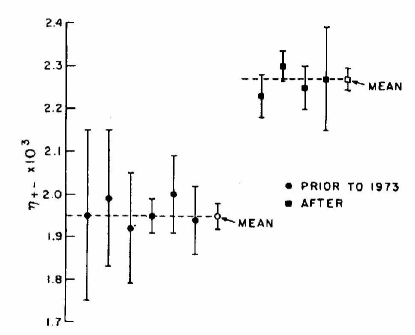
Figure 1: Measurements of $\mid\eta_{+-}\mid$ in order of their year of publication. Reprinted with permission from A. Franklin, “Forging, cooking, trimming, and riding on the bandwagon,” Am. J. Phys. 52, 786-793 (1984), copyright 1984, American Association of Physics Teachers.

Henrion and Fischhoff graphed experimental reports on the speed of light, as a function of the year of the experiment. Their graph (Fig. 2) shows that experimental results tend to cluster around a certain value for many years, and then suddenly jump to cluster around a new value, often many error bars from the previously accepted value HenrionFischhoff . Two such jumps occur for the speed of light. Again, the bias is clearly present in the graph, but the exact mechanism by which it occured is harder to discern.

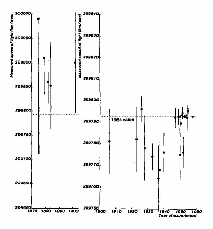
Figure 2: Measurements of the speed of light, as a function of the year of the experiment. Note that the vertical scale is changed at 1900, to make the errors bars visible. Reprinted with permission from M. Henrion and B. Fischhoff, “Assessing uncertainty in physical constants,” Am. J. Phys. 54, 791-798 (1986), copyright 1986, American Association of Physics Teachers.

V Results that are too good to be true

Newton’s results on the speed of sound, and Millikan and Cameron’s results on cosmic rays, are in retrospect too good to be true, because they were working with deficient or incorrect theories. But even results that agree with correct theories can be too good to be true.

Henrion and Fischhoff looked at the reported values for a number of other fundamental constants, and with one exception, found that error bars had been systematically underestimated—results were more spread about the correct value than they should have been, based on the reported error bars HenrionFischhoff . Underestimating error bars is not necessarily a sign of experimenter bias. However, their one exception is. Unlike the fundamental constants such as $\hbar$ or $c$, for which there are no theoretical calculations to tell experimenters what to expect, experiments measuring the ratio of the absolute ohm to the ohm as maintained by the National Bureau of standards ($\Omega_{ABS}/\Omega_{NBS}$) “should” obtain one, if all calibrations are correct. Henrion and Fischhoff found that the experimental results for $\Omega_{ABS}/\Omega_{NBS}$ were too closely clustered around one—given the error bars reported, the chance was only 1 in 200 that the results would be so clustered together. This indicates that experimenters, knowing that they should obtain one, somehow biased their measurements or calculations to get “the right answer.”

We depart briefly from physics to consider a famous case from biology. Fisher’s reexamination of Mendel’s results in his famous experiments on heredity in peas, showed that Mendel’s results were simply too good to be true. Many of his results show ratios that almost exactly match the theoretical values, with deviations much smaller than the expected statistical fluctuations. Fisher showed that only 3 experiments in 100,000 would obtain results as close to theory as Mendel’s MendelFisher ; MendelNote . This has often been taken as proof of fraud, either on the part of Mendel, or an assistant, but no evidence of fraud has been found, other than the fact that the data is too good to be true. As we have seen, such biases can arise in a number of ways without intentional fraud. For example, Root-Bernstein has shown that the results can be explained if Mendel was unconsciously biased in cases where the assignation of pea traits was ambiguous MendelRoot . Olby has pointed out that the results could be explained if Mendel kept track of the ratios as he collected data, and stopped recording when the ratios were what he expected MendelOlby ; MendelOlbyNote .

VI Other cases

Experimenter biases can also arise from ambiguities in when to discard data. If equipment was clearly malfunctioning during a run, data can no longer be used. But it will sometimes be unclear whether data should be discarded, and in ambiguous cases, whether the data agrees with expectations may unconsciously (or consciously) tip the experimenter in one direction or another. One of the most (in)famous cases is that of Millikan’s oil drop experiments, where he both demonstrated the quantization of charge, and measured this quantized charge MillikanOilDrop . In his paper he claimed “It is to be remarked, too, that this is not a selected group of drops but represents all of the drops experimented on during 60 consecutive days. . .” MillikanOriginal . But later inspection of his lab notebook shows that he threw out results for a number of oil drops, in many cases after calculating their charge. For some oil drops the equipment was clearly malfunctioning. For others, the data failed certain consistency checks. And for a few drops, Millikan simply discarded them because the calulated charges were too far off from what he believed to be the correct value. The exclusion of the latter data points appears to cross the line into fraud, but the reasons used to discard data form a continuum from obviously reasonable to fraudulent, and illustrate the difficulty in determining when it is appropriate to discard data. (Fraud is, of course, also a way in which experimenter beliefs can influence their results, but discussion of such cases is beyond the scope of this paper.)

Here we have only discussed the ways in which theoretical beliefs can affect the actual results reported. Once the results are reported, theoretical beliefs can also affect how the results are interpreted, and whether they are believed and/or published. We will not discuss such cases here, except to note that it is not always easy to separate the cases where theoretical beliefs have affected the experiment, and when they have merely affected its interpretation. The difficulty of this distinction is well-illustrated by an episode in the development of the kinetic theory of gasses.

In 1859 the scientific understanding of heat was still uncertain, and the atomic picture for materials was still controversial. Maxwell considered his now-famous model of a gas as a collection of billiard balls (atoms) undergoing elastic collisions, and came up with a startling result—he showed that with this model, the viscosity of a gas would be independent of its density MaxwellKinetic . This was surprising, since he and his colleagues, naturally, expected the viscosity to go to zero as the density went to zero. Maxwell asked Stokes about this, and Stokes assured him that experiments by Sabine on the damping of pendulums in air had demonstrated that the viscosity of air went to zero at low densities—apparently, a strong disconfirmation of the billiard ball model! Nevertheless, Maxwell continued his investigations, and eventually did experiments showing that gas viscosity was constant over a wide range of densities. With this triumph of the billiard ball model, Stokes went back and reanalyzed Sabine’s experiment. Stokes came to realize that, in fact, his previous analysis of Sabine’s experiment has implicitly assumed that the viscosity was proportional to density at low densities, thus assuming the result he claimed to be proving. It could be argued that this is not a case where theory affected reported experimental results, but merely one where it affected the way in which results were interpreted; but the line is blurry, for Stokes and Maxwell both apparently believed that “the viscosity goes to zero as the density goes to zero,” was the experimental result.

We have seen that there are a number of ways in which the theoretical expectations of physicists can influence their results. This bias is certainly less prominent than in fields such as psychology and medicine, but it is clearly present, and important if we want to understand how physics works in practice. Finally, if the reader knows of any cases of expectation bias, either historical or recent, in their own fields, I’d love to hear about them!

- (1) Sir A. C. Doyle, A Scandal in Bohemia, in Sherlock Holmes: The Complete Illustrated Short Stories (Chancellor Press, Great Britain, 1985), p. 12.
- (2) Sir Arthur Eddington, New Pathways in Science (The University of Michigan Press, 1959), p.211.
- (3) The photographs were crude forgeries, produced by two young girls, using cutouts from a magazine, and freehand drawings. J. Randi, Flim-Flam! Psychics, ESP, Unicorns, and Other Delusions (Prometheus Books, Buffalo, New York, 1982).
- (4) S. G. Brush, “The role of history in the teaching of physics,” Phys. Teach. 7, 271-280 (1969).
- (5) M. A. B. Whitaker, “History and quasi-history in physics education: part I,” Phys. Educ. 14, 108-112 (1979).
- (6) A. Wróblewski, “de Mora Luminis: A spectacle in two acts with a prologue and an epilogue,” Am. J. Phys. 53, 620-630 (1985).
- (7) G. Holton, “Einstein, Michelson, and the ‘crucial’ experiment,” Isis 60, 132-197 (1969).
- (8) A. Van Helden, “Saturn and his anses,” J. Hist. Astro. 5, 105-121 (1974).
- (9) M. J. Nye, “N-rays: an epsisode in the history and psychology of science,” Hist. Stud. Phys. Sci. 11, 125-156 (1980).
- (10) I. Langmuir, “Pathological Science,” Colloquium at Knolls Research Laboratory, 18 Dec 1953, ed. R. N. Hall; reprinted in Phys. Today, 42, 36-48 (1989).
- (11) W. F. Brewer, B. L. Lambert, “The theory-ladenness of observation and the theory-ladenness of the rest of the scientific process,” Phil. Sci. 68, S176-182 (2001).
- (12) W. J. Bisson and W. H. Dennen, “Newton and spectral lines,” Sci. 135, 921-922 (1962).
- (13) E. G. Boring, “Newton and the spectral lines,” Sci. 136, 600-601 (1962).
- (14) J. V. Narlikar and S. Bhate, “Search for ancient Indian records of the sighting of supernovae,” Current Sci. 81, 701-705 (2001).
- (15) E. F. Redish, Teaching Physics (John Wiley and Sons, U.S.A., 1993), p.130-132.
- (16) R. F. Gunstone and R. T. White, “Understanding of gravity,” Sci. Educ. 65, 291-299 (1981).
- (17) R. Rosenthal, “How often are our numbers wrong?,” Am. Psychol. 33, 1005-1008 (1978).
- (18) R. Rosenthal, Experimenter Effects in Behaviour Research, enlarged ed. (Irvington Pub. Inc., New York, 1976).
- (19) J. Worrall, “The pressure of light: the strange case of the vacillating ‘cruical experiment’,” Stud. Hist. Phil. Sci. 13, 133-171 (1982). This has citations to the original experiments and presents a fascinating history of other light pressure experiments.
- (20) A. Franklin, Selectivity and Discord: Two Problems of Experiment (University of Pittsburgh Press, Pittsburgh, 2002), chapter 6.
- (21) P. Galison, How Experiments End (University of Chicago Press, Chicago, 1987).
- (22) P. Galison, ibid., p.85 (Table 3.2).
- (23) R. S. Westfall, “Newton and the Fudge Factor,” Science 179, 751-758 (1973).
- (24) F. S. Crawford Jr., Waves (Mc-Graw-Hill Publishing Co., New York, 1968), p. 167. Crawford writes “Now comes the interesting question: How could Newton come so close to the right answer (which shows that something is right with his derivation) and yet miss it by 15% (which shows that something is wrong with his derivation)?”
- (25) T. S. Kuhn, “The caloric theory of adiabatic compression,” Isis 49, 132-140 (1958).
- (26) T. S. Kuhn, “The function of measurement in modern physical science,” Isis 52, 161-193 (1961).
- (27) R. Fox, The Caloric Theory of Gases: From Lavoisier to Regnault (Oxford University Press, Claredon, 1971), p.162-5.
- (28) Laplace’s derivation of a factor of in the speed of sound was valid despite his use of caloric theory, but his method of calculating the value of from the experimental results of Delaroche and Berard was not.
- (29) Particle Data Group: S. Eidelman, et. al. “Review of particle properties,” Phys. Lett. B 592, 1-1109 (2004), p.16-18.
- (30) Particle Data Group: R. K. Kelly, et. al., “Review of particle properties,” Rev. Mod. Phys. 52, S1-286 (1980), p.S284-286.
- (31) A. Franklin, “Forging, cooking, trimming, and riding on the bandwagon,” Am. J. Phys. 52, 786-793 (1984).
- (32) M. Henrion and B. Fischhoff, “Assessing uncertainty in physical constants,” Am. J. Phys. 54, 791-798 (1986).
- (33) R. A. Fisher, “Has Mendel’s work been rediscovered?,” Ann. Sci. 1, 115-137 (1936).
- (34) A number of authors have also taken issue with Fisher’s statistical arguments, although few find enough problems with Fisher’s analysis to conclude that Mendel’s data are unproblematic.
- (35) R. S. Root-Bernstein, “Mendel and methodology,” Hist. Sci. 21, 275-295 (1983).
- (36) R. C. Olby, The Origins of Mendelism (Schocken Books, New York, 1966), p.182-185.
- (37) Root-Bernstein has pointed out a logical flaw in Olby’s evidence that such optional stopping occured, but is also unable to rule it out as a possible mechanism MendelRoot .
- (38) S. G. Brush, The Kind of Motion we Call Heat: A History of the Kinetic Theory of Gases in the 19th Century, Book 1 (North-Holland Publishing Co., Amsterdam, 1976), p.189-191.
- (39) G. Holton, “Subelectrons, presuppositions, and the Millikan-Ehrenhaft Dispute,” Hist. Stud. Phys. Sci. 9, 161-224 (1978).
- (40) R. A. Millikan, “On the elementary electrical charge and the Avogadro constant,” Phys. Rev. 2, 109-143 (1913), p.138.