The two electron molecular bond revisited: from Bohr orbits to two-center orbitals

Abstract

Niels Bohr originally applied his approach to quantum mechanics to the H atom with great success. He then went on to show in 1913 how the same “planetary-orbit” model can predict binding for the H₂ molecule. However, he misidentified the correct dissociation energy of his model at large internuclear separation, forcing him to give up on a “Bohr’s model for molecules”. Recently, we have found the correct dissociation limit of Bohr’s model for H₂ and obtained good potential energy curves at all internuclear separations. This work is a natural extension of Bohr’s original paper and corresponds to the $D=\infty$ limit of a dimensional scaling (D-scaling) analysis, as developed by Herschbach and coworkers.

In a separate but synergetic approach to the two-electron problem, we summarize recent advances in constructing analytical models for describing the two-electron bond. The emphasis here is not maximally attainable numerical accuracy, but beyond textbook accuracy as informed by physical insights. We demonstrate how the interplay of the cusp condition, the asymptotic condition, the electron-correlation, configuration interaction, and the exact one electron two-center orbitals, can produce energy results approaching chemical accuracy. To this end, we provide a tutorial on using the Riccati form of the ground state wave function as a unified way of understanding the two-electron wave function and collect a detailed account of mathematical derivations on the exact one-electron two-center wave functions. Reviews of more traditional calculational approaches, such as Hartree-Fock, are also given.

The inclusion of electron correlation via Hylleraas type functions is well known to be important, but difficult to implement for more than two electrons. The use of the D-scaled Bohr model offers the tantalizing possibility of obtaining electron correlation energy in a non-traditional way.

I Introduction

I.1 Overview

We are in the midst of a revolution at the interface between chemistry and physics, largely due to the interplay between quantum optics and quantum chemistry. For example, the explicit control of molecules afforded by modern femtosecond lasers and adaptive computer feedback Juds92 has opened new frontiers in molecular science. In such studies, molecules are controlled by sculpting the amplitude and phase of femtosecond pulses, forcing the molecule into predetermined electronic and rotational-vibrational states. This holds great promise for vital applications, from the trace detection of molecular impurities, such as dipicolinic acid as it appears in anthrax PNAS , to the utilization of molecular excited states for quantum information storage and retrieval Niel99 .

We are thus motivated to rethink certain aspects of molecular physics and quantum chemistry especially with regard to the excited state dynamics and coherent processes of molecules. The usual discussions of molecular structure are based on solving the many-particle Schrödinger equation with varying degree of sophistication, from exacting Diffusion Monte Carlo methods, coupled cluster expansion, configuration interactions, to density functional theory. All are intensely numerical. Despite these successful tools of modern computational chemistry, there remains the need for understanding electron correlations in some relatively simple way so that we may describe excited states dynamics with reasonable accuracy.

In this work, we propose to reexamine these questions in two complementary ways. One approach is based on the recently resurrected Bohr’s model for molecules Svid04 ; Svid05 . In particular, we show that by modifying the original Bohr’s model Bohr1 in a simple way, specially when augmented by dimensional scaling (D-scaling), we can describe both the singlet and triplet potential of H₂ with remarkable accuracy (see Figs. 2, 5).

In another approach, following the lead of the French school of Le Sech Le ; Sech96 , we use correlated two-center orbitals of the H${}_{2}^{+}$ molecule to model H₂’s ground and excited state. This approach worked well, even when only a simple electron correlation function is used, see Table 1.

Table 1: The binding energy of H₂ molecule based on “exact” two-center H${}_{2}^{+}$ orbitals.

Orbital Binding energy (eV) No Free Parameter 1 Free (screening) parameter Jaffé (VI.55) 4.50 4.60 Hylleraas (VI.58) 4.51 4.62

When we allow the $\alpha$ and $B$ parameters of Eqs. (VI.55) and (VI.58) to vary, we obtain a binding energy of 4.7 eV. The binding energy is comparable to the experimental value of 4.7 eV.

The Bohr model and D-scaling technique taken together with good (uncorrelated) molecular orbitals is especially interesting and promising. As discussed in subsection C, the Bohr model yields a good approximation to the electron-electron Coulomb energy, which can be used to choose a renormalized nuclear charge and a much improved (correlated) two electron wave function.

Figure 1: Cylindrical coordinates (top) and electronic distances (bottom) in H₂ molecule. The nuclei $Z$ are fixed at a distance $R$ apart. In the Bohr model, the two electrons rotate about the internuclear axis $z$ with coordinates $\rho_{1}$, $z_{1}$ and $\rho_{2}$, $z_{2}$ respectively; the dihedral angle $\phi$ between the ($\rho_{1},z_{1}$) and ($\rho_{2},z_{2}$) planes remains constant at either $\phi=\pi$ or $\phi=0$. The sketch corresponds to configuration 2 of Fig. 2, with $\phi=\pi$.

I.2 The Bohr molecule

Figure 1 displays the Bohr model for a hydrogen molecule Bohr1 ; Svid04 ; Svid05 , in which two nuclei with charges $Z|e|$ are separated by a fixed distance $R$ (adiabatic approximation) and the two electrons move in the space between them. The model assumes that the electrons move with constant speed on circular trajectories of radii $\rho_{1}=\rho_{2}=\rho$. The circle centers lie on the molecule axis $z$ at the coordinates $z_{1}=\pm z_{2}=z$. The separation between the electrons is constant. The net force on each electron consists of three contributions: attractive interaction between an electron and the two nuclei, the Coulomb repulsion between electrons, and the centrifugal force on the electron. We proceed by writing the energy function $E=T+V$, where the kinetic energy $T=p_{1}^{2}/2m+p_{2}^{2}/2m$ for electrons 1 and 2 can be obtained from the quantization condition that the circumference is equal to the integer number $n$ of the electron de Broglie wavelengths $2\pi\rho=nh/p$, so that we have $T=p^{2}/2m=n^{2}\hbar^{2}/2m\rho^{2}$; the unit of distance is taken to be the Bohr radius $a_{0}=\hbar^{2}/me^{2}$, and the unit of energy the atomic energy, $e^{2}/a_{0}$ where $m$ and $e$ are, respectively, the mass and charge of the electron. The Coulomb potential energy $V$ is given by

$$V=-\frac{Z}{r_{a1}}-\frac{Z}{r_{b1}}-\frac{Z}{r_{a2}}-\frac{Z}{r_{b2}}+\frac{1}{r_{12}}+\frac{Z^{2}}{R},$$ (I.1)

where $r_{ai}$ ($i=1,2$) and $r_{bi}$ are the distances of the $i$th electron from nuclei A and B, as shown in Fig. 1 (bottom), $r_{12}$ is the separation between electrons. In cylindrical coordinates the distances are

$$r_{ai}=\sqrt{\rho_{i}^{2}+\left(z_{i}-\frac{R}{2}\right)^{2}},\quad r_{bi}=\sqrt{\rho_{i}^{2}+\left(z_{i}+\frac{R}{2}\right)^{2}},$$

$$r_{12}=\sqrt{(z_{1}-z_{2})^{2}+\rho_{1}^{2}+\rho_{2}^{2}-2\rho_{1}\rho_{2}\cos\phi},$$

here $R$ is the internuclear spacing and $\phi$ is the dihedral angle between the planes containing the electrons and the internuclear axis. The Bohr model energy for a homonuclear molecule having charge $Z$ is then given by

$$E=\frac{1}{2}\left(\frac{n_{1}^{2}}{\rho_{1}^{2}}+\frac{n_{2}^{2}}{\rho_{2}^{2}}\right)+V(\rho_{1},\rho_{2},z_{1},z_{2},\phi).$$ (I.2)

Possible electron configurations correspond to extrema of the energy function (I.2). For $n_{1}=n_{2}=1$ the energy has extrema at $\rho_{1}=\rho_{2}=\rho$, $z_{1}=\pm z_{2}=z$ and $\phi=\pi$, $0$. These four configurations are pictured in Fig. 2 (upper panel). For example, for configuration 2, with $z_{1}=-z_{2}=z$, $\phi=\pi$, the extremum equations $\partial E/\partial z=0$ and $\partial E/\partial\rho=0$ read

$$\frac{Z(R/2-z)}{\left[\rho^{2}+(R/2-z)^{2}\right]^{3/2}}+\frac{z}{4[\rho^{2}+z^{2}]^{3/2}}-$$

$$\frac{Z(R/2+z)}{\left[\rho^{2}+(R/2+z)^{2}\right]^{3/2}}=0,$$ (I.3)

$$\frac{Z\rho}{\left[\rho^{2}+(R/2-z)^{2}\right]^{3/2}}+\frac{Z\rho}{\left[\rho^{2}+(R/2+z)^{2}\right]^{3/2}}-$$

$$\frac{\rho}{4[\rho^{2}+z^{2}]^{3/2}}=\frac{1}{\rho^{3}},$$ (I.4)

which are seen to be equivalent to Newton’s second law applied to the motion of each electron. Eq. (I.3) specifies that the total Coulomb force on the electron along the $z-$axis is equal to zero; Eq. (I.4) specifies that the projection of the Coulomb force toward the molecular axis equals the centrifugal force. At any fixed internuclear distance $R$, these equations determine the constant values of $\rho$ and $z$ that describe the electron trajectories. Similar force equations pertain for the other extremum configurations.

In Fig. 2 (lower panel) we plot $E(R)$ for the four Bohr model configurations (solid curves), together with “exact” results (dots) obtained from extensive variational calculations for the singlet ground state ${}^{1}\Sigma_{g}^{+}$, and the lowest triplet state, ${}^{3}\Sigma_{u}^{+}$ Kolo60 . In the model, the three configurations 1, 2, 3 with the electrons on opposite sides of the internuclear axis ($\phi=\pi$) are seen to correspond to the ${}^{1}\Sigma_{g}^{+}$ singlet ground states, whereas the other solution 4 with the electrons on the same side ($\phi=0$) corresponds to the first excited, ${}^{3}\Sigma_{u}^{+}$ triplet state. At small internuclear distances, the symmetric configuration 1 originally considered by Bohr agrees well with the “exact” ground state quantum energy; at larger $R$, however, this configuration’s energy rises far above that of the ground state and ultimately dissociates to the doubly ionized limit, 2H⁺+2e. In contrast, the solution for the asymmetric configuration 2 appears only for $R>1.20$ and in the large $R$ limit dissociates to two H atoms. The solution for asymmetric configuration 3 exists only for $R>1.68$ and climbs steeply to dissociate to an ion pair, H${}^{+}+$H^-. The asymmetric solution 4 exists for all $R$ and corresponds throughout to repulsive interaction of two H atoms.

Figure 2: Energy $E(R)$ of H₂ molecule for four electron configurations (top) as a function of internuclear distance $R$ calculated within the Bohr model (solid lines) and the “exact” ground ${}^{1}\Sigma_{g}^{+}$ and first excited ${}^{3}\Sigma_{u}^{+}$ state energy of Ref. Kolo60 (dots). Unit of energy is 1 a.u.$=27.21$ eV, and unit of distance is the Bohr radius.

We then extend these “Bohr molecule” studies in several ways. In particular, we use a variant of the dimensional scaling (D scaling) theory as it was originally developed in quantum chromodynamics and applied with great success to molecular and statistical physics Witt80 ; Hers92 . This is based on an analysis in which the usual kinetic energy terms in the Schrödinger equation are written in D dimensions, i.e.,

$$-\frac{\hbar^{2}}{2m}\sum_{i=1}^{3}\frac{\partial^{2}}{\partial x_{i}^{2}}\rightarrow-\frac{\hbar^{2}}{2m}\sum_{i=1}^{D}\frac{\partial^{2}}{\partial x_{i}^{2}}$$ (I.5)

This provides another avenue into the interface between the old (Bohr-Sommerfeld) and the new (Heisenberg-Schrödinger) quantum mechanics. In particular, when $D\rightarrow\infty$ the two electron Schrödinger equation can be scaled and sculpted into a form which is when $D\rightarrow\infty$ identical to the Bohr theory of the H₂ molecule, and much better than when $1/D$ or other corrections are included.

I.3 Simple correlation energy from the Bohr model

The Bohr model offers an effective way to treat most of the correlation energy absent in the conventional Hartree–Fock (HF) approximation. Here we show how a charge renormalization method can be applied to improve the ground state energy obtained in the HF approximation. We start from He-like ions and consider a nucleus with charge $Z$ and two electrons moving around it. According to the Bohr model the ground state energy is given by the minimum of the following expression

$$E=\frac{1}{2}\left(\frac{1}{\rho_{1}^{2}}+\frac{1}{\rho_{2}^{2}}\right)-\frac{Z}{\rho_{1}}-\frac{Z}{\rho_{2}}+\frac{1}{\sqrt{\rho_{1}^{2}+\rho_{2}^{2}-2\rho_{1}\rho_{2}\cos\phi}},$$ (I.6)

where $\phi$ is the dihedral angle between electrons. At the minimum $\phi=\pi$ and Eq. (I.6) reduces to

$$E=\frac{1}{2}\left(\frac{1}{\rho_{1}^{2}}+\frac{1}{\rho_{2}^{2}}\right)-\frac{Z}{\rho_{1}}-\frac{Z}{\rho_{2}}+\frac{1}{\rho_{1}+\rho_{2}}.$$ (I.7)

Optimization with respect to $\rho_{1}$ and $\rho_{2}$ yields

$$\rho_{1}=\rho_{2}=\frac{1}{Z-\frac{1}{4}},\qquad E_{B}=-\left(Z-\frac{1}{4}\right)^{2}.$$ (I.8)

The HF approximation in the framework of the Bohr model means that optimum parameters $\rho_{1}$ and $\rho_{2}$ are determined by minimization of Eq. (I.7) with no electron repulsion term, i.e., omitting the electron-electron correlation. In the HF approximation the Bohr model gives

$$\rho_{1}=\rho_{2}=\frac{1}{Z},\qquad E_{\text{B-HF}}=-Z^{2}+\frac{Z}{2}.$$ (I.9)

For the He atom ($Z=2$) we obtain $E_{\text{B-HF}}=-3$ a.u., while $E_{B}=-3.0625$ a.u. Thus, the inclusion of correlation shifts the ground state energy down by

$$E^{{\rm B}}_{\text{corr}}=-\frac{1}{16}=-0.0625\text{ a.u.}$$ (I.10)

The Bohr model itself is quasiclassical and, as a consequence, it predicts the He ground state energy with only $5.4\%$ accuracy ($E_{\text{exact}}=-2.9037$ a.u.). However, the Bohr model provides a quantitative way to include the correlation energy. Let us consider the He ground state energy calculated using the HF (effective charge) variational wave function

$$\Psi(r_{1},r_{2})=C\exp[-\tilde{Z}(r_{1}+r_{2})],$$ (I.11)

where $\tilde{Z}$ is a variational parameter (effective charge), which is determined by minimizing the energy $E=\tilde{Z}^{2}-2Z\tilde{Z}+5\tilde{Z}/8$, $\tilde{Z}=Z-5/16.$ The wave mechanical HF energy is

$$E^{{\rm W}}_{\text{HF}}=-\left(Z-\frac{5}{16}\right)^{2}.$$ (I.12)

For $Z=2$ we obtain $E^{{\rm W}}_{\text{HF}}=-2.8476$ a.u. The difference between $E^{{\rm W}}_{\text{HF}}$ and the exact value is due to the correlation energy missing in the HF treatment. One can notice that if we add the correlation energy (I.10) to $E^{{\rm W}}_{\text{HF}}$ we obtain

$$E^{{\rm W}}_{\text{HF}}+E^{{\rm B}}_{\text{corr}}=-2.9101\text{ a.u.,}$$

which substantially improves the answer and deviates by only $0.2\%$ from the exact value. Such an idea can be incorporated by renormalization of the nuclear charge Kais93 . Let us define an effective charge $Z_{\text{eff}}$ by the condition

$$E_{\text{B-HF}}(Z_{\text{eff}})=E^{{\rm W}}_{\text{HF}}(Z),$$ (I.13)

which yields

$$Z_{\text{eff}}=\frac{1}{4}+\sqrt{\frac{1}{16}+\left(Z-\frac{5}{16}\right)^{2}}.$$ (I.14)

The effective charge improves the Bohr model energy by taking into account the difference between the quasiclassical and fully quantum mechanical description. The effective charge is calculated from the correspondence between the Bohr model in the HF approximation and the quantum mechanical HF answer. Now, if we take the Bohr model energy $E_{B}(Z)$ (I.8) (that includes correlation) but with $Z_{\text{eff}}$ instead of $Z$ it improves the quantum mechanical HF answer:

$$E_{B}(Z_{\text{eff}})=-\left(Z-\frac{5}{16}\right)^{2}-\frac{1}{16}=E^{{\rm W}}_{\text{HF}}(Z)-\frac{1}{16}.$$ (I.15)

The correction energy $-1/16$ is independent of $Z$ and coincides with Eq. (I.10). Table 2 compares the quantum mechanical HF answer for the ground state energy of He-like ions and the improved value (I.15). Depending on $Z$ Eq. (I.15) improves the accuracy $10-20$ times.

Table 2: Ground state energy of the He-like ions in the HF approximation $E^{{\rm W}}_{\rm HF}$ and the value improved by the Bohr model $E_{B}$. The last two columns compare the accuracy of the HF and the improved result.

$Z$	$E^{{\rm W}}_{\text{HF}}(Z)$	$Z-Z_{\text{eff}}$	$E_{B}(Z_{\text{eff}})$	$E_{\text{exact}}$	$\Delta E_{\text{HF}},\text{ \%}$	$\Delta E_{B}(Z_{\text{eff}}),\text{ \%}$
2	-2.8476	0.0441	-2.9101	-2.9037	1.93	0.22
3	-7.2226	0.0508	-7.2851	-7.2799	0.79	0.072
4	-13.597	0.0540	-13.6602	-13.6555	0.42	0.033
5	-21.9726	0.0558	-22.0351	-22.0309	0.26	0.019
6	-32.3476	0.0570	-32.4102	-32.4062	0.18	0.012
7	-44.7226	0.0578	-44.7852	-44.7814	0.13	0.008
8	-59.0976	0.0584	-59.1602	-59.1566	0.10	0.006
9	-75.4726	0.0589	-75.5352	-75.5317	0.08	0.004
10	-93.8476	0.0592	-93.9102	-93.9068	0.06	0.003

I.4 Correlated two-center orbitals

¿From the preceding discussion it is clear that we need good (hopefully simple) HF wave functions. There is, of course, a great deal of work on this problem but we find the two-center orbital approach of Le Sech and coworkers ABB ; A-FL ; SL ; Le ; Sech96 and of Patil PTT to be especially useful. In a previous publication ScullyEtAl , we attempted a first principle (semi-tutorial) presentation employing that the exact two-center orbitals obtained from solving the Schrödinger equation for the H${}_{2}^{+}$ ion. As shown by Le Sech these are the most useful building blocks for constructing the electronic wave functions of the homonuclear H₂ molecule. One simple form of the electronic ground state constructed with two-center orbitals is

$$\Psi_{{\rm H}_{2}}(1,2)=\Psi_{{\rm H}_{2}^{+},1\sigma}(1)\Psi_{{\rm H}_{2}^{+},1\sigma}(2)\chi_{00}\left(1+\frac{1}{2}r_{12}\right),$$ (I.16)

where $\Psi_{{\rm H}_{2}^{+},1\sigma}$ is the solution of the Schrödinger equation for the H${}_{2}^{+}$ in prolate-spheroidal (ellipsoidal) coordinates, $\chi_{00}=[|\uparrow_{1}\downarrow_{2}\rangle-|\downarrow_{1}\uparrow_{2}\rangle]/\sqrt{2}$ is singlet spin function, and $(1+\frac{1}{2}r_{12})$ is the Hylleraas correlation factor. See more detailed discussions of (I.16) in Sections IV–VI below. This wave function yields a binding energy of 4.5 eV for H₂ molecule without any variational parameters. Variation with respect to a couple of parameters in the function (I.16) shifts the binding energy to 4.7 eV, giving remarkable agreement with the experimental value. To achieve the same result, sums over many one-centered atomic orbitals or Hylleraas type of wave function (cf. (IV.30) below) that explicitly include the interelectronic distance are usually used. This has been demonstrated by the earlier work of Kolos and Wolniewicz KW . Kolos and Szalewicz KS , and that of James and Coolidge james , respectively.

In these studies the introduction of a correlation factor, taking into account the Coulomb interaction between the two electrons, is naturally motivated by considering the trial wave function as broken into three parts, we write

$$\Psi(r_{1},r_{2})=\Psi(r_{1})\Psi(r_{2})f(r_{1},r_{2}),$$ (I.17)

where $\Psi(r_{1})$ and $\Psi(r_{2})$ are exact one electron solutions in the absence of interaction between electrons. For $\Psi(r_{1},r_{2})$ the Schrödinger equation (in atomic units) gives

$$\Psi(r_{2})f(r_{1},r_{2})\left(-\frac{\nabla_{1}^{2}}{2}-\frac{Z_{a}}{r_{a1}}-\frac{Z_{b}}{r_{b1}}\right)\Psi(r_{1})+\Psi(r_{1})f(r_{1},r_{2})\left(-\frac{\nabla_{2}^{2}}{2}-\frac{Z_{a}}{r_{a2}}-\frac{Z_{b}}{r_{b2}}\right)\Psi(r_{2})\\ +\Psi(r_{1})\Psi(r_{2})\left(-\frac{\nabla_{1}^{2}}{2}-\frac{\nabla_{2}^{2}}{2}+\frac{1}{r_{12}}\right)f(r_{1},r_{2})+\mbox{cross terms}\\ =\left(E-\frac{Z_{a}Z_{b}}{R}\right)\Psi(r_{1})\Psi(r_{2})f(r_{1},r_{2})\,.$$ (I.18)

where cross terms mean terms that go as $\nabla_{1}\Psi(r_{1})\cdot\nabla_{1}f(r_{1},r_{2})$, etc. The solution with only the first two terms is just that for H${}_{2}^{+}$. The functions $\Psi(r_{1})$ and $\Psi(r_{2})$ exponentially decay at large distances from the nuclei. The third term corresponds to the Schrödinger equation for two free electrons,

$$\left(-\frac{\nabla_{1}^{2}}{2}-\frac{\nabla_{2}^{2}}{2}+\frac{1}{r_{12}}\right)f(r_{1},r_{2})=\varepsilon f(r_{1},r_{2})$$ (I.19)

that is the solution to Eq. (I.19) is well known Landau and is given in terms of Coulomb wave functions, i.e., confluent hypergeometric functions (see more detailed discussions in Subsection V.B), which yields the $(1+r_{12}/2)$ Hylleraas factor as an asymptotic at small $r_{12}$. In order to place this part of the present review in perspective and be ready for the paradigm shift from the old quasi quantum-mechanical Bohr model to the new fully wave-mechanical Schrödinger–Born–Oppenheimer model, we next give a brief history of the molecular orbital concepts and computations.

I.5 Context

Molecular quantum chemistry is a fascinating success story in the annals of 20th Century science. In 1926, Schrödinger introduced the all-important wave equation which soon bore his name. In the following year Schrödinger’s new theory was applied to the simplest molecular systems of the hydrogen molecular ion H${}^{+}_{2}$ by Burrau Bur and to the hydrogen molecule H₂ by Heitler and London Heit27 and Condon Con . In the same year, Born and Oppenheimer BO published their important paper dealing with molecular nuclear motion. Further, in 1928, Hund and Mulliken HM presented their venerable molecular orbital (MO) theory, which provided a powerful computational tool for chemistry and a foundation for the subsequent development of modern molecular science.

Diatomic molecules such as H₂ and HeH⁺ are the simplest of all molecules. Their analysis, modeling and computation constitute the bedrock of the study of chemical bonds in molecular structures. To quote a recent insightful article by Cotton and Nocera CN :

“It can be said without fear of contradiction that the two-electron bond is the single most important stereoelectronic feature of chemistry.”

Indeed, the description of the covalent bond in diatomics, based on the methods of Heitler–London and Hund–Mulliken, is one of the crowning achievements of quantum mechanics and fundamental physics.

Computational quantum chemistry dawned in 1927 with the advent of the Heitler–London method. However, the accuracy of these early numerical results were not satisfactory, as can be seen from the following quotation (Hinchliffe (Hin, , p. 254)):

“The calculated bond length and dissociation energy [of MO theory] are in poor agreement with experiment than those obtained from simple VB [valence bond] treatment (Table 15.3), and this puzzled many people at the time. It has also led them to believe that the VB method was the correct way forward for the description of molecular structure $\ldots$ .”

New ideas were then proposed to improve the numerical accuracy of the Heitler–London and Hund–Mulliken method. The first idea of configuration interaction (CI) is to incorporate excited states into the wave function. The second idea of correlation introduces explicit dependence of the interelectronic distance in the wave function. The idea of correlation was first demonstrated by Hylleraas hylleraas in 1929 for the helium atom and by James and Coolidge james in 1933 for H₂. The use of configuration interaction and correlation are key evolutionary steps in improving the original ideas of Heitler–London and Hund–Mulliken. We can quote the following from Rychlewski Ryc :

“$\ldots$ Very soon it has been realized that inclusion of interelectronic distance into the wave function is a powerful way of improving the accuracy of calculated results $\ldots$ . Today, methods based on explicitly correlated wave functions are capable of yielding the “spectroscopic” accuracy in molecular energy calculations (errors less than the orders of one $\mu$ Hartree) $\ldots$ .”

For more than two electrons, it is difficult for most numerical methods to include electron correlations directly except in Monte Carlo simulations. When it is possible, as in the two electron case, excellent results can be achieved with very compact wave functions.

Molecular calculations are inherently more difficult than atomic calculations. The fundamental difficulty is well stated by Teller and Sahlin teller :

“The molecular problem has a greater inherent complexity than the corresponding atomic problem…. In atoms, degeneracy due to spherical symmetry causes many levels to have nearly the same energy. This grouping of levels is responsible for the presence of a shell structure in atoms, and this shell structure is in turn the primary reason for the striking and simple behavior of atoms and the consequent successes of the independent-electron approximation for atomic systems. In passing from atoms to molecules the symmetry is reduced and the amount of degeneracy for the electronic levels becomes smaller, and, as a consequence, the power of the independent-particle model is decreased relative to the atomic case.”

Nothing illustrates this loss of symmetry, and its consequent loss of validity of the independent-particle picture better than the complete failure of the molecular orbital picture to account for the correct dissociation energy of H₂. At large internuclear separation, the symmetry is greatly reduced, and the independent occupation of single-particle molecular orbitals fails catastrophically. This failure can of course be averted by configuration-interaction, but this extra work makes it plain that molecular problems are inherently more complicated than atomic problems. Fortunately, for the investigation of ground and excited molecular states near equilibrium, one is far from the dissociation limit; the loss of symmetry complicates the calculation of the molecular orbital, but the independent particle model remains a good approximation.

In the case of H₂, a natural candidate is the orbital of the two-center one-electron molecular ion. Such orbitals will be referred to as diatomic orbitals (DO) or, in more complicated cases, shielded diatomic orbitals (SDO) when shielding is a factor to be considered. The early (1930s) ansatz wave functions of James and Coolidge james are expressed in terms of prolate spheroidal coordinates of the two electrons with respect to the two centers of the diatomic nuclei. However, their wave functions are not DOs in that they are not expansions of the exact one electron H${}_{2}^{+}$ states. Rather, their approach is CI with a basis conveniently chosen for numerical evaluation. Their work is the forerunner of the Polish quantum chemistry group Kolo60 ; KW ; KS of Kolos, Wolniewicz, etc., which have achieved the highest accuracy in numerical computation of two-electron molecules. The high accuracy obtained by Kolos and Wolniewicz in KW is admirable, but as noted by Patil, Tang and Toennies PTT ,

“$\ldots$ It is, however, perhaps somewhat unfortunate that these very impressive accomplishments have largely discouraged further fundamental studies on novel approaches to obtain accurate wave functions more directly $\ldots$ .”

A similar comment was made much earlier by Mulliken Mul :

“[T]he more accurate the calculations become the more concepts tend to vanish into thin air.”

Thus the human quest for comprehension remains, and the recent research on novel approaches to obtain accurate wave functions have indeed yielded accurate, physically motivated, and compact two-electron wave functions. Patil et al. Klei98 ; pat ; K ; Pati00 ; Pati03a ; Pati03 have advocated the construction of coalescense wave functions by incorporating both cusp and asymptotic conditions. We have provided a detailed review with simplfied derivations of this development in Section III. The other approach is the use of diatomic orbitals. Historically, the original idea of using DOs as basis for diatomic molecules seems to begin from the work of Wallis and Hulburt WH . More extensive references and history can be found in the works of Mclean, Weiss and Yoshimine mclean , Teller and Sahlin teller and Shull shull . Wallis and Hulburt’s result was not particularly successful, because there was no explicit electron correlation and solving the two-center wave function was difficult. According to Aubert, Bessis and Bessis (ABB, , Part I, p. 51):

“$\ldots$ the use of these functions, i.e., diatomic orbitals (DOs), within the one-configuration molecular-orbital scheme has not been very successful, owing to the difficulty of taking into account the interelectronic interactions and, moreover, owing to the complexity of calculations.”

The calculation of H${}_{2}^{+}$ wave function improved over the years, culminating in the extensive tabulations by Teller and Sahlin teller . In 1974–75, Aubert, Bessis and Bessis published a three-part series ABB detailing how to determine SDOs for diatomic molecules. These three papers emphasize the determination of shielded DOs. Surprisingly, the use of DO with correlation to study H₂ was not undertaken until 1981 by Aubert–Frécon and Le Sech A-FL . Le Sech, et al. have since then made further refinements to the method (Siebbeles and Le Sech SL , Le Sech Le ).

Our study of the DO’s approach was motivated by our strong interest in the modeling and computation of molecules. We were especially attracted by DOs as a natural and accurate description of chemical bonds. In Scully et al. ScullyEtAl , largely unaware of the prior work done by Aubert–Frécon and Le Sech of the French school, we obtained simple correlated DOs for diatomic molecules with good accuracy. The present paper represents part of our continued efforts in this direction. In this work, we will first study the mathematical properties of wave functions such as their cusp conditions, asymptotic behaviors, and forms of correlation functions. We summarize methods, techniques and formulas in a tutorial style, interspersed with some unpublished results of our own. It it not our intention to complete an exhaustive review on this vast subject, rather, only to record developments relevant to our interest in sufficient details. We apologize in advance for any inadvertent omissions.

I.6 Outline

The present paper is organized as follows:

• In Section II, we present some recent progress of an interpolated Bohr model.

• In Section III, we discuss some general and fundamental properties of atoms and molecules, including the Born–Oppenheimer separation, the Feynman–Hellman Theorem, Riccati form of the ground state wave function, proximal and asymptotic conditions, the coalescent construction and the dissociation limit.

• In Section IV, we introduce the basics of the 1-electron two-centered orbitals from the classic explicit solutions of Hylleraas and Jaffé. The one-centered and multi-centered orbitals will also be reviewed.

• In Section V, we present the details of the derivations of the all-important cusp conditions of Kato, and show examples as to how to verify them in prolate spheroidal coordinates. We also provide a glossary of various correlation functions that satisfy the interelectronic cusp condition.

• In Section VI, we discuss numerical modeling of diatomic molecules and compare results with the classic methods such as the Heitler–London, Hund–Muliken, Hartree–Fock and James–Coolidge, and the new approach of two-centered orbitals by Le Sech, et al.

• In Section VII we discuss alternative methods for molecular calculations based on the generalized Bohr model and the dimensional scaling.

• Finally, in Section VIII we give our conclusions and present an outlook.

II Recent progress based on Bohr’s model

The diatomic molecules in a fully quantum mechanical treatment addressed in Subsection I.E requires solution of the many-particle Schrödinger equation. However, such an approach also requires complicated numerical algorithms. As a consequence, for a few electron problem the results become less accurate and sometimes unreliable. This is pronounced for excited electron states when the application of the variational principle is much less involved. Therefore, invention of simple and, at the same time, relatively accurate methods of molecule description is quite desirable.

In this section we discuss a method which is based on the Bohr model and its modification Svid04 ; Svid05 . In particular, we show that for H₂ a simple extension of the original Bohr model Bohr1 describes the potential energy curves for the lowest singlet and triplet states just about as nicely as those from the wave mechanical treatment.

The simplistic Bohr model provides surprisingly accurate energies for the ground singlet state at large and small internuclear distances and for the triplet state over the full range of $R$. Also, the model predicts the ground state is bound with an equilibrium separation $R_{e}\approx 1.10$ and gives the binding energy as $E_{B}\approx 0.100$ a.u.$=2.73$ eV. The Heitler–London calculation, obtained from a two-term variational function, yields $R_{e}=1.51$ and $E_{B}=3.14$ eV Heit27 , whereas the “exact” results are $R_{e}=1.401$ and $E_{B}=4.74$ eV Kolo60 . For the triplet state, as seen in Fig. 2, the Bohr model gives a remarkably close agreement with the “exact” potential curve and is in fact much better than the Heitler–London result (which, e.g., is 30% higher for $R=2$). One should mention that in 1913, Bohr found only the symmetric configuration solution, which fails drastically to describe the ground state dissociation limit.

The simple Bohr model offers valuable insights for the description of other diatomic molecules. For $N$ electrons the model reduces to finding configurations that deliver extrema of the energy function

$$E=\frac{1}{2}\sum_{i=1}^{N}\frac{n_{i}^{2}}{\rho_{i}^{2}}+V({\bf r}_{1},{\bf r}_{2},...,{\bf r}_{N},R),$$ (II.1)

where the first term is the electron kinetic energy, while $V$ is the Coulomb potential energy. In such formulation of the model there is no need to specify electron trajectories nor to incorporate nonstationary electron motion. Eq. (II.1) assumes that only at some moment in time the electron angular momentum equals an integer number of $\hbar$ and the energy is minimized under this constraint. In the general case, the angular momentum of each electron changes with time; nevertheless, the total energy remains a conserved quantity.

Let us now discuss the ground state potential curve of HeH. To incorporate the Pauli exclusion principle one can use a prescription based on the sequential filling of the electron levels. In the case of HeH the three electrons can not occupy the same lowest level of HeH⁺⁺. As a result, we must disregard the lowest potential energy curve $E(R)$ obtained by the minimization of Eq. (II.1) and take the next possible electron configuration, which is shown in Fig. 3 (upper panel). For this configuration, $n_{1}=n_{2}=n_{3}=1$, however, the right energy corresponds to a saddle point rather than to a global minimum. In order to obtain the correct dissociation limit we assign the helium an effective charge $Z_{\text{He}}^{\text{eff}}=1.954$. The charge matches the difference between the exact ground state energy of the He atom and the Bohr model result. Fig. 3 shows the ground state potential curve of HeH in the Bohr model (solid curve) and the “exact” result (dots) obtained from extensive variational calculations Theo84 . The Bohr model gives a remarkably close agreement with the “exact” potential curve.

Figure 3: Energy $E(R)$ of HeH molecule for the electron configuration shown on the upper panel as a function of internuclear spacing $R$ calculated within the Bohr model for $n_{1}=n_{2}=n_{3}=1$, $Z_{He}^{\text{eff}}=1.954$ (solid line) and the “exact” ground state energy of Ref. Theo84 (dots).

II.1 Interpolated Bohr model

The original Bohr model assumes quantization of the electron angular momentum relative to the molecular axis. This yields a quite accurate description of the H₂ ground state $E(R)$ at small $R$. However, $E(R)$ becomes less accurate at larger internuclear separation as seen in Fig. 2. To obtain a better result one can use the following observation. At large $R$ each electron in H₂ feels only the nearest nuclear charge because the remaining charges form a neutral H atom. Therefore, at large $R$ the momentum quantization relative to the nearest nuclei, rather than to the molecular axis, must yield a better answer. This leads to the following expression for the energy of the H${}_{2}\,$ molecule

$$E=\frac{1}{2}\left(\frac{n_{1}^{2}}{r_{a1}^{2}}+\frac{n_{2}^{2}}{r_{b2}^{2}}\right)-\frac{Z}{r_{a1}}-\frac{Z}{r_{b1}}-\frac{Z}{r_{a2}}-\frac{Z}{r_{b2}}+\frac{1}{r_{12}}+\frac{Z^{2}}{R}$$ (II.2)

For $n_{1}=n_{2}=1$ and $R>2.8$ the expression (II.2) has a local minimum for the asymmetric configuration 2 of Fig. 2. We plot the corresponding $E(R)$ without the $1/R$ term in Fig. 4 (curve 2). At $R<2.8$ the electrons collapse into nuclei. At small $R$ we apply the quantization condition relative to the molecular axis which yields curve 1 in Fig. 4. To find $E(R)$ at intermediate separation we connect smoothly the two regions by a third order polynomial (thin line). Addition of the $1/R$ term yields the final potential curve, plotted in Fig. 5. The simple interpolated Bohr model provides a remarkably close agreement with the “exact” potential curve over the full range of $R$.

Figure 4: The Bohr model $E(R)$ for H₂ molecule without $1/R$ term. Curves 1 and 2 are obtained based on the quantization relative to the molecular axis (small $R$) and the nearest nuclei (large $R$) respectively. Thin line is the interpolation between two regions.

Figure 5: Ground state $E(R)$ of H₂ molecule as a function of internuclear distance $R$ calculated within the interpolated Bohr model (solid line) and the “exact” energy of Ref. Kolo60 (dots).

As an example of application of the interpolated Bohr model to other diatomic molecules, we discuss the ground state potential curve of LiH. The Li atom contains three electrons, two of which fill the inner shell. Only the outer electron with the principal quantum number $n=2$ is important in forming the molecular bond. This makes the description of LiH similar to the excited state of H₂ in which two electrons possess $n_{1}=1$ and $n_{2}=2$. So, we start from the H₂ excited state and apply the interpolated Bohr model as described above. Then, to obtain $E(R)$ for LiH, we take the H₂ potential curve and add the difference between the ground state energy of Li (-7.4780 a.u.) and H in the $n=2$ state, i.e., add $-7.3530$ a.u. The final result is shown in Fig. 6 (lower solid line), while dots are the “exact” numerical answer from Dock72 . One can see that the simple interpolated Bohr model provides quite good quantitative description of the potential curve of LiH, which is already a relatively complex four electron system.

Figure 6: Ground (${}^{1}\Sigma^{+}$) state energy $E(R)$ of LiH molecule as a function of internuclear distance $R$ calculated within the interpolated Bohr model (lower solid line) and the “exact” energy of Dock72 (dots). Upper solid curve is the first excited (${}^{3}\Sigma^{+}$) state energy of LiH obtained from the Bohr model ${}^{3}\Sigma^{+}_{g}$ $E(R)$ of H₂ molecule by adding the difference between the ground state energy of Li and H.

III General results and fundamental properties of wave functions

Having examined the quasi-quantum mechanical Bohr model in the preceding two sections, we now attend to the fully quantum mechanical model and its approximation and analysis.

III.1 The Born–Oppenheimer separation

The underlying theoretical basis for problems involving a few particles in atomic and molecular physics is the Schrödinger equation for the electrons and nuclei, which provides satisfactory explanations of the chemical, electromagnetic and spectroscopic properties of the atoms and molecules. Assume that the system under consideration has $N_{1}$ nuclei with masses $M_{K}$ and charges $eZ_{K},e$ being the electron charge, for $K=1,2,\ldots,N_{1}$, and $N_{2}=\sum\limits^{N_{1}}_{K=1}Z_{K}$ is the number of electrons. The position vector of the $K$th nucleus will be denoted as $\boldsymbol{R}_{K}$, while that of the $k$th electron will be $\boldsymbol{r}_{k}$, for $k=1,2,\ldots,N_{2}$. Let $m$ be the mass of the electron. The Schrödinger equation for the overall system is given by

$$H\Psi(\boldsymbol{R},\boldsymbol{r}) =\left[-\sum^{N_{1}}_{K=1}\frac{\hslash^{2}}{2M_{K}}\nabla^{2}_{K}-\sum^{N_{2}}_{k=1}\frac{\hslash^{2}}{2m}\nabla^{2}_{k}-\sum^{N_{1}}_{K=1}\sum^{N_{2}}_{k=1}\frac{Z_{K}e^{2}}{|\boldsymbol{R}_{K}-\boldsymbol{r}_{k}|}+\frac{1}{2}\sum^{N_{2}}_{\underset{\scriptstyle k,k^{\prime}=1}{k\neq k^{\prime}}}\frac{e^{2}}{|\boldsymbol{r}_{k}-\boldsymbol{r}_{k^{\prime}}|}\right.$$

$$\quad\left.+\frac{1}{2}\sum^{N_{1}}_{\underset{\scriptstyle K,K^{\prime}=1}{K\neq K^{\prime}}}\frac{Z_{K}Z_{K^{\prime}}e^{2}}{|\boldsymbol{R}_{K}-\boldsymbol{R}_{K^{\prime}}|}\right]\Psi(\boldsymbol{R},\boldsymbol{r})=E\Psi(\boldsymbol{R},\boldsymbol{r}),$$ (III.1)

where $H$ is the Hamiltonian and

$$\boldsymbol{R}=(\boldsymbol{R}_{1},\boldsymbol{R}_{2},\ldots,\boldsymbol{R}_{N_{1}}),\quad\boldsymbol{r}=(\boldsymbol{r}_{1},\boldsymbol{r}_{2},\ldots,\boldsymbol{r}_{N_{2}}).$$

The above equation is often too complex for practical purposes of studying molecular problems. Born and Oppenheimer BO provide a reduced order model by approximation, permitting a particularly accurate decoupling of the motions of the electrons and the nuclei. The main idea is to assume that $\Psi$ in (III.1) takes the form of a product

$$\Psi(\boldsymbol{R},\boldsymbol{r})=G(\boldsymbol{R})F(\boldsymbol{R},\boldsymbol{r}).$$ (III.2)

Substituting (III.2) into (III.1), we obtain

$$G(\boldsymbol{R})\left\{\left[-\sum^{N_{2}}_{k=1}\frac{\hslash^{2}}{2m}\nabla^{2}_{k}-\sum^{N_{1}}_{K=1}\sum^{N_{2}}_{k=1}\frac{Z_{K}e^{2}}{|\boldsymbol{R}_{K}-\boldsymbol{r}_{k}|}+\frac{1}{2}\sum^{N_{2}}_{\underset{\scriptstyle k,k^{\prime}=1}{k\neq k^{\prime}}}\frac{e^{2}}{|\boldsymbol{r}_{k}-\boldsymbol{r}_{k^{\prime}}|}\right]F(\boldsymbol{R},\boldsymbol{r})\right\}$$

$$\quad+\left\{\left[-\sum^{N_{1}}_{K=1}\frac{\hslash^{2}}{2M_{K}}\nabla^{2}_{K}+\frac{1}{2}\sum^{N_{1}}_{\underset{\scriptstyle K,K^{\prime}=1}{K\neq K^{\prime}}}\frac{Z_{K}Z_{K^{\prime}}e^{2}}{|\boldsymbol{R}_{K}-\boldsymbol{R}_{K^{\prime}}|}\right]G(\boldsymbol{R})\right\}F(\boldsymbol{R},\boldsymbol{r})$$

$$\quad+{\mathcal{T}}_{1}+{\mathcal{T}}_{2}=EG(\boldsymbol{R})F(\boldsymbol{R},\boldsymbol{r}),$$ (III.3)

where

$${\mathcal{T}}_{1} \equiv-G(\boldsymbol{R})\sum^{N_{1}}_{K=1}\frac{\hslash^{2}}{M_{K}}\nabla_{K}G(\boldsymbol{R})\cdot\nabla_{K}F(\boldsymbol{R},\boldsymbol{r}),$$ (III.4)

$${\mathcal{T}}_{2} \equiv-G(\boldsymbol{R})\sum^{N_{1}}_{K=1}\frac{\hslash^{2}}{2M_{K}}\nabla^{2}_{K}F(\boldsymbol{R},\boldsymbol{r}).$$ (III.5)

The essential step in the Born–Oppenheimer separation consists in dropping ${\mathcal{T}}_{1}$ and ${\mathcal{T}}_{2}$ in (III.3). This leads to the separation of the electronic wave function

$$\left(-\frac{\hslash^{2}}{2m}\sum^{N_{2}}_{k=1}\nabla^{2}_{k}+\frac{1}{2}\sum^{N_{2}}_{\underset{\scriptstyle k,k^{\prime}=1}{k\neq k^{\prime}}}\frac{e^{2}}{|\boldsymbol{r}_{k}-\boldsymbol{r}^{\prime}_{k}|}-\sum^{N_{1}}_{K=1}\sum^{N_{2}}_{k=1}\frac{Z_{K}e^{2}}{|\boldsymbol{R}_{K}-\boldsymbol{r}_{k}|}\right)F(\boldsymbol{R},\boldsymbol{r})=E_{e}(\boldsymbol{R})F(\boldsymbol{R},\boldsymbol{r}),$$ (III.6)

and a second equation for the nuclear wave function

$$\left[-\sum^{N_{1}}_{K=1}\frac{\hslash^{2}}{2M_{K}}\nabla^{2}_{K}+\frac{1}{2}\sum^{N_{1}}_{\underset{\scriptstyle K,K^{\prime}=1}{K\neq K^{\prime}}}\frac{Z_{K}Z_{K^{\prime}}e^{2}}{|\boldsymbol{R}_{K}-\boldsymbol{R}_{K^{\prime}}|}+E_{e}(\boldsymbol{R})\right]G(\boldsymbol{R})=EG(\boldsymbol{R}),$$

where $E_{e}(\boldsymbol{R})$ is the constant of separation.

In “typical” molecules, the time scale for the valence electrons to orbit about the nuclei is about once every $10^{-15}$ s (and that of the inner-shell electrons is even smaller), that of the molecular vibration is about once every $10^{-14}$ s, and that of the molecule rotation is every $10^{-12}$ s. This difference of time scale is what make ${\mathcal{T}}_{1}$ and ${\mathcal{T}}_{2}$ in (III.4) and (III.5) negligible, as the electrons move so fast that they can instantaneously adjust their motions with respect to the vibration and rotation movements of the slower and much heavier nuclei.

The Born–Oppenheimer separation breaks down in several cases, chief among them when the nuclear motion is strongly coupled to electronic motions, e.g., when the Jahn–Teller effects JT1 ; JT2 are present. It also requires corrections for loosely held electrons such as those in Rydberg atoms.

Research work on non-Born–Oppenheimer effects, the inclusion of the spin-orbit coupling, and on models without using the Born–Oppenheimer separation by treating the coupled dynamical motions of the electrons and nuclei simultaneously, may be found in Yarkony Ya1 and Öhrn Oh1 , for example.

III.2 Variational properties: the virial theorem and the Feynman–Hellman
theorem

The variational form of (III.1) is

$$\min_{\langle\Psi|\Psi\rangle=1}\langle\Psi|H|\Psi\rangle=E,$$ (III.7)

where the trial wave functions $\Psi=\Psi(\boldsymbol{R},\boldsymbol{r})$ belong to a proper function space (which is actually the Sobolev space $H^{1}({\mathbb{R}}^{3(N_{1}+N_{2})})$ in the mathematical theory of partial differential equations ((chen2, , Chapter 2))). The (unique) solution $\Psi_{0}$ attaining the minimum of $\langle\Psi|H|\Psi\rangle$ is called the ground state and the associated value $E_{0}\equiv\langle\Psi_{0}|H|\Psi_{0}\rangle$ is the corresponding ground state energy. Excited states $\Psi_{k}$ with successively higher energy levels may be obtained recursively through

$$\left.\begin{array}[]{l}\min\langle\Psi|H|\Psi\rangle\equiv E_{k}=\langle\Psi_{k}|H|\Psi_{k}\rangle,\\ \text{where $\Psi$ is subject to the constraints}\\ \langle\Psi|\Psi\rangle=1,\langle\Psi|\Psi_{0}\rangle=\langle\Psi|\Psi_{1}\rangle=\cdots=\langle\Psi|\Psi_{k-1}\rangle=0,\text{ for }k=1,2,3,\ldots~{}.\end{array}\right\}$$ (III.8)

There are two useful theorems related to the above variational formulation: the virial theorem and the Feynman–Hellman theorem. We discuss them below.

Let $\psi$ be any trial wave function. The expectation value of the kinetic energy is

$$E_{kin} \equiv\left\langle\Psi\left|-\sum^{N_{1}}_{K=1}\frac{\hslash^{2}}{2M_{K}}\nabla^{2}_{K}-\sum^{N_{2}}_{k=1}\frac{\hslash^{2}}{2m}\nabla^{2}_{k}\right|\Psi\right\rangle$$ (III.9)

Now, consider the scaling of all spatial variables by $1+\lambda$:

$$\boldsymbol{\mathcal{R}}\equiv(\boldsymbol{R},\boldsymbol{r})\longrightarrow(1+\lambda)(\boldsymbol{R},\boldsymbol{r})\equiv(1+\lambda)\boldsymbol{\mathcal{R}}.$$ (III.10)

Subject to the above transformation (III.10), we have

$$\widetilde{E}_{kin}=\frac{1}{(1+\lambda)^{2}}E_{kin}.$$

By taking the variation of $\widetilde{E}_{kin}$ with respect to $\lambda$, we see that it is the same as taking the variation of $E_{kin}$ with respect to $\Psi$. Thus

$$\frac{d}{d\lambda}\widetilde{E}_{kin}\Big{|}_{\lambda=0}=\delta E_{kin},$$

$$\frac{d}{d\lambda}\left[\frac{1}{(1+\lambda)^{2}}E_{kin}\right]\bigg{|}_{\lambda=0}=-2(1+\lambda)^{-3}\Big{|}_{\lambda=0}\cdot E_{kin}=-2E_{kin}=\delta E_{kin}.$$ (III.11)

For the potential energy, the expectation is given by

$$E_{pot}\equiv\langle\Psi|V|\Psi\rangle\equiv\langle V\rangle,$$ (III.12)

where $V$ consists of the 3 summations of Coulomb potentials inside the bracket of (III.1) (but $V$ can be allowed to be any potential whose negative gradient is force). The spatial scaling (III.10) implies the change of displacement $\delta{\mathcal{}}=\lambda{\mathcal{}}$, which is now regarded as infinitesimal. Therefore,

$$\delta E_{pot} =\frac{d}{d\lambda}\int\limits_{{\mathbb{R}}^{3N}}\psi^{*}(\boldsymbol{\mathcal{R}})V((1+\lambda)\boldsymbol{\mathcal{R}})\psi(\boldsymbol{\mathcal{R}})d\boldsymbol{\mathcal{R}})\Big{|}_{\lambda=0}$$

$$=\int\limits_{{\mathbb{R}}^{3N}}\psi^{*}(\boldsymbol{\mathcal{R}})[\boldsymbol{\mathcal{R}}\cdot\nabla V(\boldsymbol{\mathcal{R}})]\psi(\boldsymbol{\mathcal{R}})d\boldsymbol{\mathcal{R}}$$

$$=\langle\boldsymbol{\mathcal{R}}\cdot\nabla V\rangle\equiv\text{Virial},$$ (III.13)

where Virial is the quantum form of the classical virial. For $\Psi=\Psi_{0}$, the variational form (III.7) demands that

$$\delta\langle H\rangle=\delta E_{kin}+\delta E_{pot}=0.$$ (III.14)

Substituting (III.11) and (III.13) into (III.14), we obtain

$$-2E_{kin}+\text{Virial}=0.$$ (III.15)

This is the general form of the virial theorem for an isolated system of an atom or a molecule. In the particular case that

$$V(\boldsymbol{\mathcal{R}})=-\sum^{N_{1}}_{K=1}\sum^{N_{2}}_{k=1}\frac{Z_{k}e^{2}}{|\boldsymbol{R}_{K}-\boldsymbol{r}_{k}|}+\frac{1}{2}\sum^{N_{2}}_{\underset{\scriptstyle k,k^{\prime}=1}{k\neq k^{\prime}}}\frac{e^{2}}{|\boldsymbol{r}_{k}-\boldsymbol{r}_{k^{\prime}}|}+\frac{1}{2}\sum^{N_{1}}_{\underset{\scriptstyle K,K^{\prime}=1}{K\neq K^{\prime}}}\frac{Z_{K}Z_{K^{\prime}}e^{2}}{|\boldsymbol{R}_{K}-\boldsymbol{R}_{K^{\prime}}|},$$

which is the power law ${\mathcal{R}}^{n}$ (where ${\mathcal{R}}$ is the distance) with $n=-1$, the classical virial property holds:

$$\text{Virial }=nE_{pot}=-E_{pot}$$ (III.16)

as

$$\boldsymbol{\mathcal{R}}\cdot\nabla{\mathcal{R}}^{n}=(n{\mathcal{R}}^{n-1})\boldsymbol{\mathcal{R}}\cdot\nabla{\mathcal{R}}=n{\mathcal{R}}^{n}.$$

¿From (III.15) and (III.16), we obtain the virial theorem for an (exact, not trial) wave function:

$$2E_{kin}+E_{pot}=0,$$ (III.17)

or

$$E_{kin}=-\frac{1}{2}E_{pot}.$$ (III.18)

This property is used as a check for accuracy of calculations and the properness of the choices of trial wave functions.

The next, Feynman–Hellman theorem, shows how the energy of a system varies when the Hamiltonian changes.

Assume that the Hamiltonian of an atom or molecule system depends on a parameter $\alpha$, $H=H(\alpha)$. For example, $\alpha$ may represent the internuclear distance of the molecular ion H${}_{2}^{+}$. The exact wave function $\Psi=\Psi(\alpha)$ also depends on $\alpha$, so does the energy of the system $E=E(\alpha)$. Let’s see how $E(\alpha)$ changes with respect to $\alpha$, i.e.,

$$dE(\alpha)/d\alpha =\frac{d}{d\alpha}\int\Psi^{*}(\alpha)H(\alpha)\Psi(\alpha)d\boldsymbol{r}$$

$$=\int\frac{\partial\Psi^{*}(\alpha)}{\partial\alpha}H(\alpha)\Psi(\alpha)d\boldsymbol{r}+\int\Psi^{*}(\alpha)\frac{\partial H(\alpha)}{\partial\alpha}\Psi(\alpha)d\boldsymbol{r}+\int\Psi^{*}(\alpha)H(\alpha)\frac{\partial\Psi(\alpha)}{\partial\alpha}d\boldsymbol{r}$$

$$=E(\alpha)\int\frac{\partial\Psi^{*}(\alpha)}{\partial\alpha}\Psi(\alpha)d\boldsymbol{r}+\int\Psi^{*}(\alpha)\frac{\partial H(\alpha)}{\partial\alpha}\Psi(\alpha)d\boldsymbol{r}+E(\alpha)\int\Psi^{*}(\alpha)\frac{\partial\Psi(\alpha)}{\partial\alpha}d\boldsymbol{r}$$

$$=E(\alpha)\frac{d}{d\alpha}\langle\Psi(\alpha)|\Psi(\alpha)\rangle+\int\Psi^{*}(\alpha)\frac{\partial H(\alpha)}{\partial\alpha}\Psi(\alpha)d\boldsymbol{r}$$

$$=\left\langle\Psi(\alpha)\left|\frac{\partial H(\alpha)}{\partial\alpha}\right|\Psi(\alpha)\right\rangle$$

as $\langle\Psi(\alpha)|\Psi(\alpha)\rangle=1$ and is independent of $\alpha$. The above is the Feynman–Hellman theorem. Its advantage is that oftentimes $\partial H(\alpha)/\partial\alpha$ is of a very simple form. For example, for the H${}_{2}^{+}$-like equation (IV.13), upon taking $\alpha=R$ we have

$$\frac{\partial H}{\partial R}=-\frac{Z_{a}Z_{b}}{R^{3}}{\bf R+}\frac{Z_{b}{\bf r}_{b}}{r_{b}^{3}}\qquad$$

and the average force on the nucleus B is

$${\bf F}=-\frac{\partial E}{\partial R}=\frac{Z_{a}Z_{b}}{R^{3}}{\bf R-}\left\langle\frac{Z_{b}{\bf r}_{b}}{r_{b}^{3}}\right\rangle.\qquad$$

That is the force and, hence, the potential energy curve requires calculation of $\left\langle Z_{b}{\bf r}_{b}/r_{b}^{3}\right\rangle$ only. This substantially simplifies the problem since the matrix element from the $\nabla^{2}$ is no longer necessary.

III.3 Fundamental properties of one and two-electron wave functions

III.3.1 Riccati form, proximal and asymptotic conditions

In this subsection, we introduce the Riccati form of the ground state wave functions as a unified way of understanding and deriving various cusp, asymptotic and correlation functions. This forms the basis by which compact wave functions for diatomic molecules can be derived. Consider the Schrödinger equation with a spherically symmetric potential in reduced units,

$$-\frac{1}{2\mu}\nabla^{2}\psi({\bf r})+V(r)\psi({\bf r})=E\psi({\bf r}),$$ (III.19)

where $\mu=1$ is the central-force case, and $\mu=\frac{1}{2}$ is

the equal-mass, relative coordinate case. We will be primary

interested in

$$V_{c}(r)=-\frac{Z}{r},\quad\text{(cf.\ \eqref{eq2.12} below)}$$ (III.20)

however, the long range Coulomb potential is special in many ways and we can best understand the Coulomb-potential wave function by comparing and contrasting it to the short-range, Lennard-Jones potential

$$V_{LJ}(r)=\epsilon_{0}\left(\frac{1}{r^{12}}-\frac{1}{r^{6}}\right).$$ (III.21)

Since the ground state of (III.19) is strictly positive and spherically symmetric, it can always be written as (unnormalized)

$$\psi(r)={\rm e}^{-S(r)}.$$ (III.22)

Substituting this into (III.19) gives the Riccati equation for $S(r)$

$$\frac{1}{2\mu}\nabla^{2}S(r)-\frac{1}{2\mu}\nabla S(r)\cdot\nabla S(r)+V(r)=E_{0}.$$ (III.23)

Since $\nabla S(r)=S\,^{\prime}(r)\hat{\bf r}$ and $\nabla\cdot\hat{\bf r}=2/r$, we have simply,

$$\frac{1}{2\mu}S^{\,\prime\prime}+\frac{1}{\mu r}{S^{\,\prime}}-\frac{1}{2\mu}(S^{\,\prime})^{2}+V(r)=E_{0}.$$ (III.24)

The advantage of this equation is that since the RHS is a constant $E_{0}$, all the singularities of $V(r)$ must be cancelled by the derivatives of $S(r)$. In particular, if we are only seeking an approximate ground state, then a reasonable criterion would be to require $S(r)$ to cancel the most singular term in $V(r)$. For both the Coulomb and the Lennard-Jones case, the potential is most singular as $r\rightarrow 0$. We will refer to this as the proximal limit. For both cases, the singularity of $V(r)$ is only polynomial in $r$ and therefore we can assume

$$S(r)=ar^{n},$$ (III.25)

giving explicitly

$$\frac{1}{2\mu}an(n+1)r^{n-2}-\frac{1}{2\mu}a^{2}n^{2}r^{2n-2}+V(r)=E_{0}.$$ (III.26)

Note the structure of this equation, if the $V(r)$ has a repulsive polynomial singularity, then it can always be cancelled by the $r^{2n-2}$ term, leaving a less singular term $r^{n-2}$ behind. For example, in the Lennard-Jones case, the most singular term is cancelled if we set

$$-\frac{1}{2\mu}a^{2}n^{2}r^{2n-2}+\frac{\epsilon_{0}}{r^{12}}=0,$$ (III.27)

yielding, $n=-5$, and for $\mu=\frac{1}{2}$, the famous McMillan correlation function for quantum liquid helium,

$$S(r)=\frac{1}{5}\sqrt{\epsilon_{0}}\,r^{-5}.$$

However, if $V(r)$ has an attractive singularity, then it can only be cancelled by the $r^{n-2}$ term, and if $n\leq 0$, would leave behind a more singular term instead. This means that an attractive potential $V(r)$ cannot be as singular, or more singular, than $-1/r^{2}$, otherwise, the Schrödinger equation has no solutions. Fortunately, for the the Coulomb attraction (III.20), the $-Z/r$ singularity can be cancelled by setting

$$\frac{1}{2\mu}an(n+1)r^{n-2}-\frac{Z}{r}=0,$$ (III.28)

yielding, for $\mu=1$, $n=1$,

$$S(r)=Zr.$$

For electron-electron repulsion with $\mu=\frac{1}{2}$ and $Z=-1$, we would have instead

$$S(r)=-\frac{1}{2}r.$$

In the Coulomb case, these proximal conditions are known as cusp conditions. A more thorough treatment of the cusp condition for the general case will be given in Subsection V.A and Appendices F and H. The proximal criterion of cancelling the leading singularity of $V(r)$ can be applied generally to any $V(r)$. The cusp conditions are just special cases for the Coulomb potential. Note that in (III.28), the Coulomb singularity is actually cancelled only by the $S\,^{\prime}/(\mu r)$ term of the Riccati equation,

$$\frac{1}{\mu r}{S^{\,\prime}}-\frac{Z}{r}=0,$$

since requiring $S\,^{\prime}$ to be a constant at the singular point forces $S\,^{\prime\prime}=0$. Thus the cusp condition can be stated most succinctly in term of the Riccati function $S(r)$: wherever the nuclear charge is located, the radial derivative of $S(r)$ at that point must be equal to the nuclear charge.

Next, we consider the asymptotic limit of $r\rightarrow\infty$. In the case of short range potential, such that $V(r)\rightarrow 0$ faster than $1/r$, we can just completely ignore $V(r)$ in (III.24). Substituting in

$$S(r)=\alpha r+\beta\ln(r)$$

gives

$$-\frac{1}{2\mu}\frac{\beta}{r^{2}}-\frac{1}{2\mu}\left(\alpha+\frac{\beta}{r}\right)^{2}+\frac{1}{\mu r}\left(\alpha+\frac{\beta}{r}\right)=E_{0}.$$ (III.29)

The constant terms determine

$$\alpha=\sqrt{-2\mu E_{0}}=\sqrt{2\mu|E_{0}|}.$$

Setting the sum of $1/r$ terms zero gives,

$$\frac{1}{\mu r}\alpha(1-\beta)=0,$$ (III.30)

which fixes $\beta=1$. The remaining terms will decay faster than $1/r$ and can be neglected in the large $r$ limit. Thus the asymptotic wave function for any short-ranged potential (decays faster than $1/r$) must be of the form

$$\psi(r)\rightarrow\frac{1}{r}{\rm e}^{-\alpha r}.$$ (III.31)

However, for the Coulomb potential $-{\tilde{Z}}/{r}$ (we wish to reserve the possibility that $\tilde{Z}$ can be distinct from $Z$ and unrelated to $E_{0}$), we must retain it among the $1/r$ terms in (III.30),

$$\frac{1}{\mu r}\alpha(1-\beta)-\frac{\tilde{Z}}{r}=0,$$ (III.32)

resulting in

$$\beta=1-\frac{\mu\tilde{Z}}{\alpha}.$$ (III.33)

Thus the general asymptotic wave function for a Coulomb potential has a slower decay,

$$\psi(r)\rightarrow\frac{1}{r^{\beta}}{\rm e}^{-\alpha r}.$$ (III.34)

For a single electron in a central Coulomb field, $\mu=1$, $\tilde{Z}=Z$, $\alpha=Z$, $\beta=0$, and

$$\psi(r)\rightarrow{\rm e}^{-Zr},$$ (III.35)

the decay is the slowest, very different from (III.31). For more than one electron, or more than one nuclear charge, $\alpha\neq\tilde{Z}$, $\beta$ does not vanish and the correct asymptotic wave function is (III.34). We tend to forget this fact because we are too familiar with the single-electron wave function, which is the exception, rather than the norm.

The proximal and asymptotic conditions are very stringent constraints: wave functions that can satisfy both are inevitably close to the exact wave functions. Satisfying the proximal condition alone is sufficient to guarantee an excellent approximate ground state for all radial symmetric potentials such as the Lennard-Jones, the Yukawa $(V=\frac{1}{r}e^{-\alpha r},\alpha>0)$, and the Morse potential $(V=e^{-2\alpha r}-2e^{-\alpha r},\,\alpha>0)$. Needless to say, the proximal condition alone determines the exact ground state for the Coulomb and the harmonic oscillator potential. The significance of the proximal condition has always been recognized. The current interest pat in deriving compact wave functions for small atoms and molecules is based on a renewed appreciation of the importance of the correct asymptotics wave functions.

III.3.2 The coalescence wave function

Consider the case of two electrons orbiting a central Coulomb field,

$$\left(-\frac{1}{2}\nabla^{2}_{1}-\frac{1}{2}\nabla^{2}_{2}-\frac{Z}{r_{1}}-\frac{Z}{r_{2}}+\frac{1}{r_{12}}\right)\psi(r_{1},r_{2})=E\psi(r_{1},r_{2}).$$ (III.36)

Imagine that we assemble this atom one electron at a time. When we bring in the first electron, its energy is $E_{1}=-Z^{2}/2$, with wave function $\psi(r_{1})=\exp(-Zr_{1})$ localizing it near the origin. When electron 2 is still very far away, we can write the two-electron wave function as

$$\psi(r_{1},r_{2})={\rm e}^{-Zr_{1}-S(r_{2})}.$$ (III.37)

Substituting this into (III.36) yields the Riccati equation for $S(r_{2})$,

$$\frac{1}{2}S^{\,\prime\prime}-\frac{1}{2}(S^{\,\prime})^{2}+\frac{1}{r_{2}}{S^{\,\prime}}-\frac{Z}{r_{2}}+\frac{1}{r_{12}}=E_{0}+\frac{1}{2}Z^{2}.$$ (III.38)

The RHS defines the second electron’s energy, $E_{2}\equiv E_{0}+\frac{1}{2}Z^{2}$, whose magnitude is just the first removal or ionization energy. Since electron 2 is far away, and electron 1 is close to the origin, $r_{12}\approx r_{2}$. Thus electron 2 “sees” an effective Coulomb field $-\tilde{Z}/r_{2}$ with $\tilde{Z}=Z-1$. This is the case envisioned in (III.32) with $\alpha=\sqrt{-2E_{2}}$. The asymptotic wave function for the second electron is, therefore,

$$\psi(r_{2})\rightarrow r_{2}^{-\beta}{\rm e}^{-\alpha r_{2}},$$ (III.39)

with $\beta=1-(Z-1)/\alpha$. Since $\beta$ is always less than one, the $r_{2}^{-\beta}$ term is only a minor correction. Its effect can be accounted for by slightly altering $\alpha$. The important point here is that the second electron need not have the same Coulomb wave function as the first electron. This coalescence scenario would suggest, after symmetrizing (III.37), the following two-electron wave function:

$$\psi(r_{1},r_{2})={\rm e}^{-Zr_{1}-\alpha r_{2}}+{\rm e}^{-\alpha r_{1}-Zr_{2}}.$$ (III.40)

For the case where there are more than two electrons, one can imagine building up the atom or molecule sequentially one electron at a time. Each electron would then acquire a different Coulomb-potential wave function. This sequential, or coalescence scenario of approximating the ground state, in many cases, resulted in better wave functions than considering all the electrons simultaneously, which is the traditional Hartree–Fock point of view; see Subsection VI.C. In the case of He, the simple effective charge approximation

$$\psi(r_{1},r_{2})={\rm e}^{-Z_{\rm eff}r_{1}}{\rm e}^{-Z_{\rm eff}r_{2}}$$

with

$$Z_{\rm eff}=Z-\frac{5}{16}=1.6875,$$ (III.41)

gives $E_{var}=-Z_{\rm eff}^{2}=-2.8476$, while the “exact” value is -2.9037. The standard HF wave function of the form

$$\psi(r_{1},r_{2})=\phi(r_{1})\phi(r_{2})$$

improvesparr the energy to $E_{var}=-2.8617$. For comparison, the coalescent wave function (III.40) can achieve $E_{var}=-2.8674$ at $\alpha=1.286$. Patil pat , by restricting $\alpha$ to be consistent with the output variational energy via $\alpha=\sqrt{-2E_{var}-4}$, obtained $E_{var}=-2.8671$ at $\alpha=1.317$. All these values of $\alpha$ are very close to the exact asymptotic value of $\alpha=\sqrt{-2E_{2}}=\sqrt{2(0.9037)}=1.344$, lending credence to the coalescence construction. For arbitrary $Z$, by approximating $E_{0}$ by $-Z_{\rm eff}^{2}$, we can estimate $\alpha$ by

$$\alpha=\sqrt{2Z_{\rm eff}^{2}-Z^{2}}\quad(\,\approx Z-5/8\,).$$ (III.42)

For $Z=2$, this gives $\alpha=1.30$ (for small $Z$, we need to use the full expression rather than the approximation), an excellent estimate. This obviates the need for Patil’s self-consistent procedure to determine $\alpha$, and produces even slightly better results. The coalescent wave function (III.40) with this choice for $\alpha$, defines a set of parameter-free two-electron wave functions for all $Z$. The resulting energy for $Z=2-10$ is given in Table 3.

In 1930, Eckart eckart has used wave functions of the form

$$\psi(r_{1},r_{2})={\rm e}^{-ar_{1}-br_{2}}+{\rm e}^{-br_{1}-ar_{2}}$$ (III.43)

to compute the energy of a two-electron Z-atom. His resulting energy functional is

$$E_{Eck}(Z,a,b)=-Z(a+b)+\frac{1}{1+C(a,b)}\left[K(a,b)+\frac{1}{2}(a^{2}+b^{2})+ab\,C(a,b)\right],$$ (III.44)

where

$$K(a,b)=\frac{ab}{a+b}+\frac{a^{2}b^{2}}{(a+b)^{3}}+\frac{20a^{3}b^{3}}{(a+b)^{5}}\quad{\rm and}\quad C(a,b)=\frac{64a^{3}b^{3}}{(a+b)^{6}}.$$ (III.45)

He obtained an energy minimum $-2.8756613$ for He at $a=2.1832$ and $b=1.1885$. (We have used his energy expression to re-determine the energy minimum more accurately.) While the improvement in energy is a welcoming contribution, it seems difficult to interpret the resulting wave function physically. How can an electron “sees” a nucleus with charge greater than 2?

To gain further insight into Eckart’s result, and coalescence wave function in general, we note that (III.43) can be rewritten as

$$\chi(r_{1},r_{2})={\rm e}^{-A(r_{1}+r_{2})}\cosh\left[B(r_{1}-r_{2})\right],$$ (III.46)

with $A=(a+b)/2$ and $B=(a-b)/2$. This form has the HF part ${\rm e}^{-A(r_{1}+r_{2})}$. If we substitute Eckart’s values, we see that $A=(2.1832+1.1885)/2=1.6859$, which is nearly identical to the effective charge value (III.41). This is not accidental. If we use the approximation (III.42) for $\alpha$, then the coalescence wave function (III.40) would automatically predict

$$A=\frac{1}{2}(Z+\alpha)=Z-\frac{5}{16}\,!$$ (III.47)

Thus within the class of Eckart wave function (III.43), the coalescence scenario correctly predicts the path of optimal energy as being along $A=Z_{\rm eff}$. Moreover, this improvement in energy, which has laid dormant in Eckart’s result for three quarters of a century, can now be understood as due to the radial correlation cosh term in (III.46), built-in automatically by the coalescence construction. This term is the smallest (=1) when $r_{1}=r_{2}$, but is large when the separation $r_{1}-r_{2}$ is large, i.e., it encourages the two electrons to be separated in the radial direction.

This suggests that we should reexamine Eckart’s energy functional in terms of parameters $A$ and $B$. Expanding (III.44) to fourth order in $B$ yields,

$$E_{Eck}(Z,A,B)=-Z_{\rm eff}^{2}+(A-Z_{\rm eff})^{2}-\frac{3}{8}y+\frac{3}{2}y^{2}-\frac{1}{2A}y^{2},$$ (III.48)

where $y\equiv B^{2}/A$. If $B=0$, $A=Z_{\rm eff}$ this yields the effective charge energy $-Z_{\rm eff}^{2}$. Regarding the effect of $B$ as perturbing on this fixed choice of $A$, the $1/A\approx 1/Z$ term can first be ignored. Minimizing $y$ simply yields

$$E_{Eck}(Z,A,B)=-Z_{\rm eff}-\frac{3}{128}-\frac{1}{128Z_{\rm eff}}$$ (III.49)

at

$$y=\frac{B^{2}}{A}=\frac{1}{8}\,,$$ (III.50)

where we have restored the $1/A$ term. This remarkably simple result is the content of Eckart’s energy functional. The energy is lower from the effective charge value by a nearly constant amount $3/128$. In column three of Table 3, we compare this approximate energy (III.49), with the absolute minimum of the Eckart’s energy functional on the fourth column. The agreement is uniformly excellent. By comparison, we see that the coalescence construction,without invoking any minimization process, also gives a very good account of the energy minimum.

Table 3: Ground state energy of the He-like ions as calculated from various wave functions.

$Z$	$E({\rm Coales})$	$E({\rm Approx.})$	$E({\rm Abs.Min.})$	$E({\rm exact})$	$f_{LS}$	$f_{PJ}$	$1+\frac{1}{2}r_{12}$
2	-2.8673	-2.8757	-2.8757	-2.9037	-2.9016(3)	-2.9017(4)	-2.8898(7)
3	-7.2355	-7.2490	-7.2488	-7.2799	-7.268(1)	-7.271(1)	-7.264(1)
4	-13.6072	-13.6232	-13.6230	-13.6555	-13.637(2)	-13.642(1)	-13.634(2)
5	-21.9802	-21.9978	-21.9975	-22.0309	-22.004(2)	-22.014(2)	-22.011(2)
6	-32.3539	-32.3725	-32.3723	-32.4062	-32.376(3)	-32.386(3)	-32.382(3)
7	-44.7280	-44.7473	-44.7471	-44.7814	-44.740(4)	-44.755(3)	-44.753(3)
8	-59.1023	-59.1221	-59.1220	-59.1566	-59.115(4)	-59.129(4)	-59.127(4)
9	-75.4768	-75.4970	-75.4969	-75.5317	-75.490(6)	-75.502(4)	-75.494(4)
10	-93.8514	-93.8719	-93.8718	-93.9068	-93.859(6)	-93.875(5)	-93.885(5)

III.3.3 Electron correlation functions

Coalescence wave functions are better than HF wave function because they have built-in radial correlations. To further improve our description of He, as first realized by Hylleraas hylleraas , one can introduce electron-electron correlation directly by forcing the two-electron wave function to depend on $r_{12}$ explicitly. (A more detailed discussion of correlation functions will be given in Subsection V.B below.) Again, our analysis is simplified by use of the Riccati function. Let

$$\psi({\bf r}_{1},{\bf r}_{2})={\rm e}^{-S(r_{1},r_{2},r_{12})},$$ (III.51)

but now consider

$$S(r_{1},r_{2},r_{12})=Zr_{1}+Zr_{2}+g(r_{12}).$$ (III.52)

We have

$$\nabla_{1}S = Z\hat{\bf r}_{1}+g^{\prime}\hat{\bf r}_{12},\nabla_{2}S=Z\hat{\bf r}_{2}+g^{\prime}\hat{\bf r}_{21},$$

$$\nabla^{2}_{1}S = \frac{2Z}{r_{1}}+\frac{2g^{\prime}}{r_{12}}+g^{\prime\prime},\nabla^{2}_{2}S=\frac{2Z}{r_{2}}+\frac{2g^{\prime}}{r_{12}}+g^{\prime\prime},$$

and (III.36) in terms of $S$ reads

$$g^{\prime\prime}+\frac{2g^{\prime}+1}{r_{12}}-(g^{\prime})^{2}-Zg^{\prime}(\hat{\bf r}_{1}-\hat{\bf r}_{2})\cdot\hat{\bf r}_{12}-Z^{2}=E_{0}.$$ (III.53)

In order to eliminate the $1/r_{12}$ singularity, we must have

$$\lim_{r_{12}\rightarrow 0}\,g^{\prime}(r_{12})=-\frac{1}{2}.$$

Thus, one can consider a series expansion for $g(r_{12})$ starting out as

$$g(r_{12})=-\frac{1}{2}r_{12}+\frac{1}{2}Cr_{12}^{2}+...$$

Keeping only up to the quadratic term, in the limit of $r_{12}\rightarrow 0$, (III.53) reads

$$3C-\frac{1}{4}-Z^{2}+O(r_{12})=E_{0}.$$

If $g(r_{12})$ were exact, the LHS above would be the constant ground state energy for all values of $r_{12}$. Inverting the argument, we can exploit this fact to determine $C$ at $r_{12}=0$, provided that we can estimate the ground state energy $E_{0}$. The simplest estimate for a two electron atom would be $E_{0}=-Z^{2}$, implying that

$$C=\frac{1}{12}.$$ (III.54)

However, since the effective charge approximation for the energy is much better, we should take instead, $E_{0}=-Z_{\rm eff}^{2}$, thus fixing

$$C=\frac{1}{12}+\frac{1}{3}(Z^{2}-Z_{\rm eff}^{2})=\frac{1}{12}+\frac{5}{24}\left(Z-\frac{5}{32}\right).$$ (III.55)

The determination of the quadratic term of $g(r_{12})$ was advanced only recently by Kleinekathofer et al. klein . (If we also improve the one-electron wave function from $\exp(-Zr)\rightarrow\exp(-Z_{\rm eff}r)$, then $C$ must go back to the value (III.54). The coefficient $C$ therefore depends on the quality of the single electron wave function.) The wave function (III.51) can now be written as

$$\psi({\bf r}_{1},{\bf r}_{2})={\rm e}^{-Zr_{1}}{\rm e}^{-Zr_{2}}f(r_{12}),$$

where

$$f(r_{12})=\exp\left[\frac{1}{2}r_{12}(1-Cr_{12})\right].$$ (III.56)

Since the above argument is only valid for small $r_{12}$, the large $r_{12}$ behavior of $f(r_{12})$ is not determined. It seems reasonable, however, barring any long range Coulomb effect, to assume

$$\lim_{r_{12}\rightarrow 0}f(r_{12})\longrightarrow{\rm constant}.$$ (III.57)

The form (III.56) can have behavior (III.57) if we just rewrite it as

$$f_{PJ}(r_{12})=\exp\left[\frac{r_{12}}{2(1+Cr_{12})}\right].$$ (III.58)

This Pade-Jastrow form has been used extensively in Monte Carlo calculations of atomic systems hamm . Alternatively, to achieve (III.57), Patil’s group pat ; klein have suggested the form

$$f_{P}(r_{12})=\frac{1}{2\lambda}({1+2\lambda}-{\rm e}^{-\lambda r_{12}});\quad\text{cf. (\ref{secV}.B.(3)) and Fig.~{}\ref{ff2},}$$ (III.59)

which has the small $r_{12}$ expansion

$$f_{P}(r_{12})=1+\frac{1}{2}r_{12}-\frac{\lambda}{4}r_{12}^{2}+\cdots~{}.$$ (III.60)

By comparing this with similar expansion of (III.56), we can identify

$$\lambda=2C-\frac{1}{2}=\frac{5}{12}\left(Z-\frac{5}{32}\right)-\frac{1}{3}.$$ (III.61)

Le Sech’s group SL have employed the form

$$f_{LS}(r_{12})=1+\frac{1}{2}r_{12}{\rm e}^{-ar_{12}},$$ (III.62)

with

$$a=\frac{1}{2}\lambda.$$

This function is not monotonic; it reaches a maximum at $r_{12}=1/a$ before level off back to unity; cf. Fig. 11 in Subsection V.B. However, this point may not be practically relevant, since most electron separations do not reach beyond the maximum. For the sake of comparison, we may use the maximum of Le Sech’s correlation function as its asymptotic limit. This is the natural thing to do because all three functions can now be characterized by their asymptotic value as $r_{12}\rightarrow\infty$ :

$$f_{PJ}(r_{12})\rightarrow\exp\left({\frac{1}{2C}}\right) \approx 1+\frac{1}{\lambda+1/2},$$

$$f_{P}(r_{12}) \rightarrow 1+\frac{1}{2\lambda},$$

$$f_{LS}(r_{12}) \rightarrow 1+{\frac{1}{{\rm e}\lambda}}.$$

Their approaches toward unity are approximately $\lambda^{-1}$, $\frac{1}{2}\lambda^{-1}$, and $\frac{1}{3}\lambda^{-1}$, respectively. Note also that as $\lambda$ increases with $Z$, the asymptotic value of $f(r_{12})$ decreases, this is the correct trend long observed in Monte Carlo calculations on atomic systems hamm . For $Z=2$, we take $C=1/2$, $\lambda=1/2$, $a=1/4$ and compare all three correlation functions in Fig. 7. Also plotted is the simple linear and quadratic forms. The simplest linear correlation function, $(1+\frac{1}{2}r_{12})$, is very distinct from the other three.

Figure 7: Comparison of three electron-electron correlation functions.

We now have all the ingredients needed to construct an optimal wave function for He. First, with the introduction of explicit electron correlation function, there is no need for the radial correlation introduced by the coalescence wave function, i.e., we are free to abandon the radial correlation function $\cosh(B(r_{1}-r_{2}))$. Second, the asymptotic form of the wave function $\exp(-\alpha r)$ should be maintained. However, this asymptotic wave function, when extended back to small $r$, violates the cusp condition. These concerns can be simultaneously alleviated by replacing the second electron’s wave function via

$${\rm e}^{-\alpha r_{2}}\rightarrow{\rm e}^{-Zr_{2}}\cosh(\beta r_{2}).$$

At small $r_{2}$, the $\cosh$ function is second order in $r_{2}$ and therefore will not affect the cusp condition. At large $r_{2}$, $\cosh(\beta r_{2})\rightarrow\exp(\beta r_{2})$, and the choice

$$\beta=Z-\alpha$$ (III.63)

will give back the correct asymptotic wave function. Upon symmetrization, we finally arrived at the following compact wave function for He:

$$\psi(r_{1},r_{2},r_{12})={\rm e}^{-Zr_{1}-Zr_{2}}\left[\cosh(\beta r_{1})+\cosh(\beta r_{2})\right]f(r_{12}).$$ (III.64)

This wave function, first derived by Le Sech hesech , satisfies all the cusp and asymptotic conditions. We fixed $\alpha$, $\beta$ and $C$ by (III.42), (III.63) and (III.55), respectively, and there are no free parameters. The only arbitrariness is the form the correlation function $f(r_{12})$. Since $f_{P}(r_{12})$ is bracketed by $f_{PJ}(r_{12})$ and $f_{LS}(r_{12})$, we only need to consider the latter two cases. For $Z=2-10$, the resulting ground state energy for the two electron atoms are given in Table 3.

III.3.4 The one-electron homonuclear wave function

The one-electron, homonuclear two-center Schrödinger equation

$$\left(-\frac{1}{2}\nabla^{2}-\frac{Z}{r_{a}}-\frac{Z}{r_{b}}\right)\psi({\bf r})=E\psi({\bf r}),$$ (III.65)

where $r_{a}=|{\bf r}+{\bf R}/2|$, $r_{b}=|{\bf r}-{\bf R}/2|$, can be solved exactly, as will be shown in Subsection IV.B below. However, its ground state wave function can also be accurately prescribed by proximal and asymptotic conditions. For $Z=1$, this is hydrogen molecular ion problem. As first pointed out by Guillemin and Zener (GZ) GZ , when $R=0$, the exact wave function is

$$\psi({\bf r})={\rm e}^{-2Zr}$$ (III.66)

and when $R\rightarrow\infty$, the exact wave function is

$$\psi({\bf r})={\rm e}^{-Zr_{a}}+{\rm e}^{-Zr_{b}}.$$ (III.67)

They, therefore, propose a wave function that can interpolate between the two,

$$\psi_{GZ}(r_{a},r_{a})={\rm e}^{-Z_{1}r_{a}-Z_{2}r_{b}}+{\rm e}^{-Z_{2}r_{a}-Z_{1}r_{b}}.$$ (III.68)

At $R=0$, $r_{a}=r_{b}=r$, one can take $Z_{1}=Z_{2}=Z$. At $R\rightarrow\infty$, one can choose $Z_{1}=Z$ and $Z_{2}=0$. At intermediate values of $R$, $Z_{1}$ and $Z_{2}$ can be determined variationally. This GZ wave function gives an excellent description GZ of the ground state of H${}_{2}^{+}$. As explained by Patil, Tang and Toennies PTT , another reason why this is a good wave function is that that (III.68) can satisfy both the cusp and the asymptotic condition. We can simplify Patil et al’s discussion by rewriting the GZ wave function, again, in the form

$$\psi_{GZ}(r_{a},r_{b})={\rm e}^{-A(r_{a}+r_{b})/2}\cosh\left[B(r_{a}-r_{b})/2\right],$$ (III.69)

when $R=0$, $A=2Z$, and when $R\rightarrow\infty$, $A=B=Z$. The imposition of the cusp condition can be done most easily in terms of the Riccati function. We, therefore, write

$$\psi_{GZ}(r_{a},r_{b})={\rm e}^{-S(r_{a},r_{b})},$$ (III.70)

with

$$S(r_{a},r_{b})=A(r_{a}+r_{b})/2-\ln(\,\cosh[B(r_{a}-r_{b})/2]\,).$$

The cusp condition at $r_{a}=0$ is then easily computed,

$$\frac{\partial S}{\partial r_{a}}\Bigl{|}_{r_{a}=0,r_{b}=R}=Z,\quad A+B\tanh(BR/2)=2Z.$$ (III.71)

One can verify that this is also the cusp condition at $r_{b}=0$. From (III.71), one sees easily that at $R=0$, $A=2Z$, and when $R\rightarrow\infty$, $A+B=2Z$. At finite $R$, the asymptotic limit $r\rightarrow\infty$ means that $r_{a}=r_{b}=r$ and the GZ wave function approaches

$$\psi_{GZ}(r_{a},r_{b})\rightarrow{\rm e}^{-Ar}.$$

On the other hand, the exact wave function must be of the form (III.34)

$$\psi(r_{a},r_{b})\rightarrow{\rm e}^{-\sqrt{2|E_{0}|}r-\beta\ln(r)},$$ (III.72)

with $\beta=1-2Z/\sqrt{2|E_{0}|}$. Since $2Z\geq\sqrt{2|E_{0}|}\geq Z$, we can estimate that at intermediate values of $R$, $\sqrt{2|E_{0}|}\approx\frac{3}{2}Z$, suggesting a negligible $\beta\approx-\frac{1}{3}$. Thus it is suffice to take

$$A\approx\sqrt{2|E_{0}|}$$ (III.73)

Guillemin and Zener have allowed both $A$ and $B$ to be variational parameters. Patil et al’s estimate PTT of $A$ is essentially that of (III.73) but with slight improvement to incorporate the variation due to $\beta\neq 0$. We adhere to the cusp condition (III.71) but allow $A$ to vary. In practice, it is easier to just let $B$ vary and fix A via the cusp condition (III.71). In all cases, this wave function can provide an excellent description of the hydrogen molecular ion, with energy derivation only on the order of $10^{-3}$ Hartree over the range of $R=0-5$.

III.3.5 The two-electron homonuclear wave function

The two-electron homonuclear Schrödinger equation is,

$$\left(-\frac{1}{2}\nabla^{2}_{1}-\frac{1}{2}\nabla^{2}_{2}-\frac{Z}{r_{1a}}-\frac{Z}{r_{1b}}-\frac{Z}{r_{2a}}-\frac{Z}{r_{2b}}+\frac{1}{r_{12}}\right)\psi({\bf r}_{1},{\bf r}_{2})=E\psi({\bf r}_{1},{\bf r}_{2}).$$ (III.74)

Let’s denote the one-electron two-center GZ wave function as

$$\phi({\bf r})={\rm e}^{-A\sigma}\cosh(B\delta)$$

where we have defined

$$\sigma=\frac{r_{a}+r_{b}}{2},\quad\delta=\frac{r_{a}-r_{b}}{2}.$$

(The variables $\sigma$ and $\delta$ here will correspond, respectively, to $\lambda$ and $\mu$ of the prolate spheroidal coordinates in Subsection IV.B.) To describe the two-electron wave function, if one were to follow the usual approach, one would begin by defining the Hartree-Fock like wave function

$$\psi({\bf r}_{1},{\bf r}_{2})=\phi({\bf r}_{1})\phi({\bf r}_{2})={\rm e}^{-A(\sigma_{1}+\sigma_{2})}\cosh(B\delta_{1})\cosh(B\delta_{2}).$$ (III.75)

However, this molecular orbital approach is well known not to give the correct dissociation limit of H₂. In the limit of $R\rightarrow\infty$, we know that

$$\phi({\bf r})\rightarrow{\rm e}^{-Zr_{a}}+{\rm e}^{-Zr_{b}}$$ (III.76)

and therefore

$$\psi({\bf r}_{1},{\bf r}_{2}) \rightarrow ({\rm e}^{-Zr_{1a}}+{\rm e}^{-Zr_{1b}})({\rm e}^{-Zr_{2a}}+{\rm e}^{-Zr_{2b}})$$ (III.77)

$$\rightarrow ({\rm e}^{-Zr_{1a}}{\rm e}^{-Zr_{2b}}+{\rm e}^{-Zr_{1b}}{\rm e}^{-Zr_{2a}})+({\rm e}^{-Zr_{1a}}{\rm e}^{-Zr_{2a}}+{\rm e}^{-Zr_{1b}}{\rm e}^{-Zr_{2b}})$$

Only the first parenthesis, the Heilter-London wave function, gives the correct energy of two well separated atoms with energy $E=2(-\frac{1}{2}Z^{2})$. The remaining parenthesis describes, in the case of H₂, the ionic configuration of H^-H⁺, which has higher energy than two separated neutral hydrogen atoms. Thus the molecular orbital approach (III.75) will alway overshoot the correct dissociation limit. This is a fundamental shortcoming of the molecular orbital approach and cannot be cured by merely improving the one-electron wave function, i.e., by use of the exact one-electron, two-center wave function. Even the coalescent construction cannot overcome this fundamental problem. In the large $R$ limit, the inner electron’s wave function must be (III.76), and hence no matter how one constructs the outer electron’s asymptotic wave function, one can never reproduces the Heilter-London wave function. In both the molecular orbital and the coalescent approach, one must resort to configuration interaction to achieve the correct dissociation limit. Even if one were to use the exact one-electron wave function in doing configuration intereaction, as it was done by Siebbeles and Le Sech SL , the energy still overshoots the correct dissociation limit if the correlation $(1+\frac{1}{2}r_{12})$ is used. This is because we must have $f(r_{12})\rightarrow const$ in order to reproduce the Heilter-London limit.

However, one can learn from Guillemin and Zener’s approach, and insist on a wave function that is correct in both the $R=0$ and $R\rightarrow\infty$ limit. This seemed a very stringent requirement, but surprisingly, it is possible. The wave function is

$$\psi({\bf r}_{1},{\bf r}_{2})={\rm e}^{-A(\sigma_{1}+\sigma_{2})}\cosh\left[B(\delta_{1}-\delta_{2})\right]f(r_{12}).$$ (III.78)

For $R=0$, $\sigma_{1}=r_{1}$, $\sigma_{2}=r_{2}$, and the above function reduces to

$$\psi({\bf r}_{1},{\bf r}_{2})={\rm e}^{-A(r_{1}+r_{2})}f(r_{12}).$$

which is not a bad description of He. In the limit of $R\rightarrow\infty$, if we take $A=B=Z$, we have

$$\psi({\bf r}_{1},{\bf r}_{2}) = ({\rm e}^{-Zr_{1a}}{\rm e}^{-Zr_{2b}}+{\rm e}^{-Zr_{1b}}{\rm e}^{-Zr_{2a}})f(r_{12}),$$ (III.79)

$$= ({\rm e}^{-Zr_{1a}}{\rm e}^{-Zr_{2b}}+{\rm e}^{-Zr_{1b}}{\rm e}^{-Zr_{2a}}),$$

since $f(\infty)\rightarrow 1$. Thus wave function (III.78) is the simplest homonuclear two electron wave function that can describe both limits adequately. The wave function (III.78) for H₂ without $f(r_{12})$ has been derived some time ago by Inui inui and Nordsieck nord . However, they were only interested in improving the wave function and energy at the equilibrium separation and were not concerned with whether the wave function can yield the correct dissociation limit.

To estimate the form of the correlation function $f(r_{12})$, we repeat our analysis as in the Helium case. The two-electron wave function can again be written in the Riccati form (III.51), but now with

$$S(r_{1},r_{2},r_{12})=Zr_{1a}+Zr_{2b}+g(r_{12}),$$ (III.80)

where we have assumed the unsymmetrized form of the Heilter-London wave function. The resulting equation for $g$ is also similar to (III.53),

$$g^{\prime\prime}+\frac{2g^{\prime}+1}{r_{12}}-(g^{\prime})^{2}-Zg^{\prime}(\hat{\bf r}_{1a}-\hat{\bf r}_{2b})\cdot\hat{\bf r}_{12}-Z^{2}+O\left(\frac{1}{R}\right)=E_{0}.$$ (III.81)

In the Helium case, the dot product term vanishes in the limit of $r_{12}\rightarrow 0$, here it does not. In the case where the two electrons meet along the molecular axis, $\hat{\bf r}_{1a}=\hat{\bf z}$, $\hat{\bf r}_{2b}=-\hat{\bf z}$, $\hat{\bf r}_{12}=-\hat{\bf z}$, the resulting equation

$$g^{\prime\prime}+\frac{2g^{\prime}+1}{r_{12}}-(g^{\prime})^{2}+2Zg^{\prime}-Z^{2}+O\left(\frac{1}{R}\right)=E_{0}$$ (III.82)

can be solved by setting $E_{0}=-Z^{2}$, and expanding

$$g(r_{12})=-\frac{1}{2}r_{12}+\frac{1}{2}Cr_{12}^{2}+...$$

In the limit of $r_{12}\rightarrow 0$, (III.82) reads

$$3C-\frac{1}{4}-Z+O(r_{12})=0,$$

giving,

$$C=\frac{Z}{3}+\frac{1}{12}.$$ (III.83)

This agrees with Patil et al’s result PTT of

$$\lambda=2C-\frac{1}{2}=\frac{1}{3}(2Z-1),$$

but without the need of consulting hypergeometric functions. For the H₂ case, $C=5/12=0.42$. In our calculation with wave function (III.78), with $f_{PJ}(r_{12})$ given by (III.58), the energy minimum at intermediate values of $R$ is at $C=0.40$, in excellent agreement with the predicted value. Since $C\approx 0.50$ for Helium, $C$’s variation with $R$ is very mild.

The resulting energy for the wave function (III.78), is given in Fig. 8 (solid line). We vary the parameter $B$, while the other parameters $A$ and $C$ are fixed by Eqs. (III.71) and (III.83). The parameter B is 0.8 for $R<2$, and moves graduately toward one at larger values of $R$. The energy at equilibrium is as good as Siebbeles and Le Sech’s calculation SL with unscaled H${}_{2}^{+}$ wave functions and correlation function $(1+\frac{1}{2}r_{12})$ (triangles). Without configuration interaction, Siebbeles and Le Sech’s energy overshot the dissociatin limit as shown. The wave function (III.78) can be further improved by adding a coalescense component à la Patil, Tang and Toennies PTT . This will be detailed in the next subsection.

Figure 8: Ground state potential curve $E(R)$ of H₂ for different trial wave functions. Triangles correspond to “Le Sech” molecular orbital calculation with exact H${}_{2}^{+}$ one-electron orbitals. Our wave function (III.78) (solid line) gives the correct dissociation limit. Patil et al.’s results are shown as small dot (function (III.88), (III.91), (III.92)) and dash (function (III.102)) lines. Large dots are “exact” values of Ref. Kolo60 .

III.3.6 Construction of trial wave functions by Patil and coworkers

The previous discussion demonstrates that relatively simple wave functions which incorporate the cusp conditions and the large distance asymptotics, having no or only a few variational parameters, can be constructed to yield fairly accurate results. Here we mention other similar trial wave functions studied in the literature. The importance of the local properties in the calculation of the chemical bond has been emphasized by Patil and coworkers K ; PTT ; P ; Pati00 ; Pati03a ; Pati03 . Their analysis is in the spirit of our previous discussion, however, yields more complicated trial wave functions. Here we briefly mention the main aspects of the construction scheme and, to be specific, consider the ground state of H₂ molecule described by the Schrödinger equation (III.74).

Let us assume that $r_{2}\gg r_{1}$, $R$, $1$. Then $r_{12}\approx r_{2a}\approx r_{2b}\approx r_{2}$ and the Hamiltonian reads

$$\hat{H}=-\frac{1}{2}\nabla_{1}^{2}-\frac{Z}{r_{1a}}-\frac{Z}{r_{1b}}+\frac{Z^{2}}{R}-\frac{1}{2}\nabla_{2}^{2}-\frac{(2Z-1)}{r_{2}}.$$ (III.84)

The first four terms in (III.84) yield the H${}_{2}^{+}$ problem, while the last two terms correspond to motion of a particle in a Coulomb potential with an effective charge $2Z-1$. This Hamiltonian allows us to separate variables and write $\Psi({\bf r}_{1},{\bf r}_{2})=\Psi_{\text{H}_{2}^{+}}({\bf r}_{1})\varphi({\bf r}_{2})$, where the function $\varphi({\bf r}_{2})$ satisfies the equation

$$\left(-\frac{1}{2}\nabla_{2}^{2}-\frac{(2Z-1)}{r_{2}}\right)\varphi({\bf r}_{2})=-\varepsilon\varphi({\bf r}_{2}),$$ (III.85)

$\varepsilon=E_{\text{H}_{2}^{+}}-E>0$ is the ionization energy of the H₂ molecule, and $E$ is the ground state energy of H₂. As a result, the asymptotic behavior of $\Psi({\bf r}_{1},{\bf r}_{2})$ at $r_{2}\gg r_{1}$, $R$, $1$, is

$$\Psi({\bf r}_{1},{\bf r}_{2})\approx r_{2}^{(2Z-1)/\sqrt{2\varepsilon}-1}\exp(-\sqrt{2\varepsilon}r_{2})\Psi_{\text{H}_{2}^{+}}({\bf r}_{1}),$$ (III.86)

which is similar to the coalescence wave function (III.39) for He. Now assume that $r_{2}\gg r_{1}\gg R$, $1$, then $\Psi_{\text{H}_{2}^{+}}({\bf r}_{1})$ is given by Eq. (III.72) and, therefore,

$$\Psi({\bf r}_{1},{\bf r}_{2})\approx r_{1}^{2Z/\sqrt{2\varepsilon_{1}}-1}r_{2}^{(2Z-1)/\sqrt{2\varepsilon}-1}\exp(-\sqrt{2\varepsilon_{1}}r_{1}-\sqrt{2\varepsilon}r_{2}),$$ (III.87)

where $\varepsilon_{1}=Z^{2}/R-E_{\text{H}_{2}^{+}}>0$ is the separation energy of electron in H${}_{2}^{+}$. The power-law factor slowly varies as compared to the exponential decaying contribution. Hence, one can assume the power-law factor to be a constant or approximate the combination $r^{a}\exp(-br)$ as

$$r^{a}\exp(-br)=\exp(-br+a\ln r)\approx\exp(-br+a\ln r_{0}+(r-r_{0})a/r_{0}),$$

where $r_{0}$ can be determined as a variational parameter or chosen to be $r_{0}=R+1/b$ PTT .

To incorporate the cusp conditions and the large distance asymptotic the trial wave function is separated into two parts

$$\Psi({\bf r}_{1},{\bf r}_{2})=\Phi({\bf r}_{1},{\bf r}_{2})f_{P}(r_{12}),$$ (III.88)

where $f_{P}(r_{12})$ is the Patil et al. electron-electron correlation function given by Eq. (III.59). Roothaan and Weiss Root60 have made a very accurate numerical investigation of the desired correlation function for the ground state of the He atom. In the vicinity of $r_{12}=0$, the correlation function is linear and satisfies the cusp condition. It monotonically increases and approaches a constant as $r_{12}$ becomes very large. Clearly the function $f_{P}(r_{12})$ satisfies these conditions (see Fig. 12). In the united atom limit $(R=0)$ it was found that the energies computed with the variationally determined $\lambda$ are essentially the same as given by the analytical expression,

$$\lambda=\frac{5}{12}Z-\frac{1}{3}$$ (III.89)

derived from a theory in which $1/r_{12}$ is treated as a perturbation K . In a molecular system, as $R$ increases, one should expect $\lambda$ to decrease monotonically and become vanishingly small for $R\rightarrow\infty$. The small and large $R$ behavior is satisfied provided Klei98

$$\lambda=\frac{5Z/6-1/3}{1+10Z^{3}R^{2}/(15Z-6)}.$$ (III.90)

The electron-nucleus cusp conditions do not uniquely define the space wave function $\Phi({\bf r}_{1},{\bf r}_{2})$. If one wishes to maintain the electronic configuration idea with an independent particle picture, one can adopt the following form of $\Phi({\bf r}_{1},{\bf r}_{2})$:

$$\Phi({\bf r}_{1},{\bf r}_{2})=\phi(r_{1})\phi(r_{2}),$$ (III.91)

with $\phi(r_{j}),$ $j=1,2,$ being the Guillemin-Zener GZ trial wave function for H${}_{2}^{+}$

$$\phi(r_{j})=\exp(-z_{1}r_{ja}-z_{2}r_{jb})+\exp(-z_{2}r_{ja}-z_{1}r_{jb}),$$ (III.92)

where $z_{1}>0,$ $z_{2}>0$ are variational parameters. Alternatively, $z_{1}$ and $z_{2}$ can be determined from the cusp conditions at $r_{ja}=0$ and $r_{jb}=0$ for $j=1,2$. The wave function (III.91), (III.92) is identical to (III.75) which is known not to give the correct dissociation limit of H₂. However, for the pedagogical reason we briefly discuss it here.

As $r_{1a}$ approaches zero

$$\Phi({\bf r}_{1},{\bf r}_{2})\rightarrow\phi(r_{2})\left[(1-z_{1}r_{1a})\exp(-z_{2}R)+(1-z_{2}r_{1a})\exp(-z_{1}R)\right].$$ (III.93)

Imposing the cusp condition $\Phi({\bf r}_{1},{\bf r}_{2})\rightarrow G(r_{2})(1-Zr_{1a})$ we obtain an equation for $z_{1}$ and $z_{2}$:

$$z_{1}=Z+(Z-z_{2})\exp[-(z_{1}-z_{2})R].$$ (III.94)

Thus, if $z_{1}$ and $z_{2}$ are related as in Eq. (III.94), then the electron-nucleus cusp conditions are automatically satisfied. The second equation for $z_{1}$ and $z_{2}$ can be determined by the asymptotic condition. For $r_{2}\gg r_{1}\gg R$, $1$ Eqs. (III.91), (III.92) yield

$$\Psi({\bf r}_{1},{\bf r}_{2})\approx\exp[-(z_{1}+z_{2})r_{1}-(z_{1}+z_{2})r_{2}].$$ (III.95)

¿From the other hand, according to Eq. (III.87), the wave function must have the following exponential behavior $\Psi({\bf r}_{1},{\bf r}_{2})\sim\exp(-\sqrt{2\varepsilon_{1}}r_{1}-\sqrt{2\varepsilon}r_{2})$. The two parameters $z_{1}$ and $z_{2}$ do not allow to match the asymptotic exactly. However, one can approximately choose Klei98

$$z_{1}+z_{2}=\varepsilon_{1}+\varepsilon=\frac{Z^{2}}{R}-E.$$ (III.96)

Eqs. (III.94), (III.96) determine $z_{1}$ and $z_{2}$ self-consistently together with the ground state energy $E$.

Kleinekathöfer et al. Klei98 used the trial function (III.88), (III.91), (III.92) with $\lambda$, $z_{1}$ and $z_{2}$ determined from Eqs. (III.90), (III.94), (III.96). The wave function has no free parameters and yields $4.661$ eV for the binding energy of the H₂ molecule which is very close to the exact value of $4.745$ eV. However, $E(R)$ becomes less accurate at large $R$ and fails to describe the dissociation limit. The corresponding $E(R)$ is shown as a small dot line (Patil et al. 1) in Fig. 8.

Both the cusp conditions and the large distance asymptotic can be satisfied exactly provided more sophisticated trial functions are introduced. For example, for small and intermediate $R$, Patil et al. PTT suggested to use a combination of “inner” and “outer” molecular orbitals which are build from the Guillemin-Zener one-electron wave functions:

$$\Psi_{m}({\bf r}_{1},{\bf r}_{2})=[\phi_{\text{in}}({\bf r}_{1})\phi_{\text{out}}({\bf r}_{2})+\phi_{\text{in}}({\bf r}_{2})\phi_{\text{out}}({\bf r}_{1})]f_{P}(r_{12}),$$ (III.97)

where the “inner” orbital is

$$\phi_{\text{in}}({\bf r}_{j})=\exp(-z_{1}r_{ja}-z_{2}r_{jb})+\exp(-z_{2}r_{ja}-z_{1}r_{jb}).$$ (III.98)

Analogously, an “outer” orbital is defined as

$$\phi_{\text{out}}({\bf r}_{j})=\exp(-z_{3}r_{ja}-z_{4}r_{jb})+\exp(-z_{4}r_{ja}-z_{3}r_{jb}).$$ (III.99)

All the parameters $z_{1}$, $z_{2}$, $z_{3}$ and $z_{4}$ are determined by the cusp and asymptotic conditions.

At large $R$, the atomic orbital wave function provides a better description of the two electron system. The appropriate wave function is PTT

$$\Psi_{a}({\bf r}_{1},{\bf r}_{2})=[\Phi({\bf r}_{1},{\bf r}_{2})+\Phi({\bf r}_{2},{\bf r}_{1})]f_{P}(r_{12}),$$ (III.100)

where

$$\Phi({\bf r}_{1},{\bf r}_{2})=\exp[-Z(r_{1a}+r_{1b}+r_{2a}+r_{2b})]\left\{\cosh(z_{5}r_{1b})\cosh(z_{6}r_{2a})+\cosh(z_{6}r_{1b})\cosh(z_{5}r_{2a})\right\}.$$ (III.101)

Eq. (III.100) satisfies all the electron-nucleus cusp conditions. At the same time, it has two free parameters $z_{5}$ and $z_{6}$ which can be used to satisfy the two asymptotic conditions.

For a description in the entire range of internuclear distances, one can use a linear combination of the two wave functions just discussed

$$\Psi=\Psi_{m}+D\Psi_{a},$$ (III.102)

where $D$ is a variational parameter. For H₂ the molecular orbital $\Psi_{m}$ dominates in the region $R<1.7$, while the atomic orbital $\Psi_{a}$ dominates at $R>1.7$. With this complicated one parameter wave function Patil et al. PTT obtained $4.716$ eV for the binding energy of H₂ molecule and a very accurate potential curve in the entire range of $R$. The corresponding $E(R)$ is shown as a dash line (Patil et al. 2) in Fig. 8. Similar wave functions which take full advantage of the asymptotic and proximal boundary conditions are useful in variational calculations of larger systems Pati03a .

IV Analytical wave mechanical solutions for one electron molecules

From now on throughout the Sections IV, V and VI, unless otherwise noted, we assume the Born–Oppenheimer separation, where there are $N$ nuclei, containing $Z_{k}$ protons located at $\boldsymbol{R}_{k}$, respectively, for $k=1,2,\ldots,N$, and $N_{e}$ electrons. Each electron’s coordinates are denoted as $\boldsymbol{r}_{j}$, $j=1,2,\ldots,N_{e}$, where $\boldsymbol{r}_{j}=(x_{j},y_{j},z_{j})$. The steady-state equation, in atomic units, can be written as

$$H\psi=E\psi,\quad H=-\frac{1}{2}\sum^{N_{e}}_{j=1}\nabla^{2}_{j}+\sum_{1\leq j<k\leq N_{e}}\frac{1}{r_{jk}}-\sum^{N_{e}}_{j=1}\sum^{N}_{k=1}\frac{Z_{k}}{|\boldsymbol{r}_{j}-\boldsymbol{R}_{k}|}+\sum_{1\leq j<k\leq N}\frac{Z_{j}Z_{k}}{|\boldsymbol{R}_{j}-\boldsymbol{R}_{k}|},$$ (IV.1)

where

$$\psi=\psi(\boldsymbol{r}_{1},\boldsymbol{r}_{2},\ldots,\boldsymbol{r}_{N_{e}}),\quad\nabla^{2}_{j}\equiv\frac{\partial^{2}}{\partial x^{2}_{j}}+\frac{\partial^{2}}{\partial y^{2}_{j}}+\frac{\partial^{2}}{\partial z^{2}_{j}},\quad r_{jk}\equiv|\boldsymbol{r}_{j}-\boldsymbol{r}_{k}|,\quad j,k=1,2,\ldots,N_{e}.$$

We wish to solve the eigenvalue problem (IV.1).

Closed-form solutions to (IV.1) are hard to come by in general. What is known today is the following:

• $\boldsymbol{N_{e}=1,N=1}$:
  This is the case of hydrogen atom H (or H-like ions with a single nucleus and electron) whose solutions are known explicitly in closed form, to be briefly reviewed in Subsection IV.1.

• $\boldsymbol{N_{e}=1,N=2}$:
  This is the H${}_{2}^{+}$ (or H${}_{2}^{+}$-like) two-centered molecular ion, whose solutions are separable and expressible as an infinite series of products of special functions in prolate spheroidal coordinates, where coefficients of the series are not explicitly given. Such are the two renowned classic solutions due to Hylleraas and Jaffé, to be discussed in Subsection IV.2.

• $\boldsymbol{N_{e}=1,N\geq 3}$:
  This one-electron multi-centered molecular ion has an analytic solution due to Shibuya and Wulfman SW in terms of integral equations on the unit hypersphere of the 4-dimensional momentum space. This will be reviewed in Subsection IV.3.

Except for Case (i) above, one must resort to numerical methods in order to derive quantitative and qualitative information, for all cases where $N_{e}\neq 1$, $N\neq 1$. Our particular interest in this paper is the diatomic case, with $N_{e}=N=2$, using the orbitals in Cases (i) and (ii) above as the building blocks.

IV.1 The hydrogen atom

When $N_{e}=N=1$, with $Z_{1}=1$ and $\boldsymbol{R}_{1}=\boldsymbol{0}$, equation (IV.1) becomes

$$\left(-\frac{1}{2}\nabla^{2}-\frac{1}{r}\right)\psi(\boldsymbol{r})=E\psi(\boldsymbol{r}),\qquad\boldsymbol{r}\in{\mathbb{R}}^{3},$$ (IV.2)

the Born–Oppenheimer separation of the hydrogen atom.

We write (IV.2) in spherical coordinates in view of the symmetry involved:

$$\frac{1}{r}\frac{\partial^{2}}{\partial r^{2}}(r\psi)+\frac{1}{r^{2}}\Lambda^{2}\psi+\frac{2}{r}\psi-2E\psi=0,$$ (IV.3)

where

$$\Lambda^{2} \equiv\frac{1}{\sin^{2}\theta}\frac{\partial^{2}}{\partial\phi^{2}}+\frac{1}{\sin\theta}\frac{\partial}{\partial\theta}\left(\sin\theta\frac{\partial}{\partial\theta}\right),\quad\text{(the Legendrian);}$$ (IV.4)

$$r =\text{the radial variable,}\qquad 0<r<\infty;$$

$$\theta =\text{the colatitude,}\qquad 0\leq\theta\leq\pi;$$

$$\phi =\text{the azimuth,}\qquad 0\leq\phi\leq 2\pi.$$

Equation (IV.2) has separable solutions

$$\psi(\boldsymbol{r})=\psi(r,\theta,\phi)=R(r)Y(\theta,\phi).$$ (IV.5)

The angular variables are quantized first as we know that angular functions are the spherical harmonics

$$Y(\theta,\phi)=Y_{\ell m}(\theta,\phi)=\Theta_{\ell m}(\theta)\Phi_{m}(\phi),\qquad\ell=0,1,2,\ldots,m=\ell,\ell-1,\ldots,-\ell,$$ (IV.6)

on the unit sphere $\mathcal{S}_{2}\equiv\{\boldsymbol{r}\in{\mathbb{R}}^{3}\mid|\boldsymbol{r}|=1\}$, satisfying

$$\Lambda^{2}Y_{\ell m}(\theta,\phi)=-\ell(\ell+1)Y_{\ell m}(\theta,\phi),$$ (IV.7)

where in (IV.6),

$$\Phi_{m}(\phi)=(2\pi)^{-\frac{1}{2}}e^{im\phi},$$ (IV.8)

$$\Theta_{\ell m}(\theta)=\left\{\frac{(2\ell+1)(\ell-|m|)!}{2(\ell+|m|)!}\right\}^{\frac{1}{2}}P^{|m|}_{\ell}(\cos\theta),$$ (IV.9)

$$(P^{|m|}_{\ell}\text{ is the associated Legendre function}).$$

Using (IV.5)–(IV.7) in (IV.2), we obtain the equation for the radial function

$$\frac{1}{r}(rR)^{\prime\prime}-\frac{\ell(\ell+1)}{r^{2}}R+\left(\frac{2}{r}-2E\right)R=0.$$ (IV.10)

Solutions to the eigenvalue problem (IV.10) that are square integrable over $0<r<\infty$ are known to be

$$R(r)=R_{n\ell}(r)=(-2)\left\{\frac{(n-\ell-1)!}{2n[(n+\ell)!]^{3}}\right\}(2r)^{\ell}L^{2\ell+1}_{n+\ell}(2r)e^{-r},$$ (IV.11)

$$E_{n}=-\frac{1}{2}\frac{1}{n^{2}},\quad n=1,2,\ldots,\text{ independent of }\ell,$$

where $L^{2\ell+1}_{n+\ell}$ are the associated Laguerre functions such that for $m,n=0,1,2,\ldots$

$$xL^{m}_{m+n}{}^{\prime\prime}+(m+1-x)L^{m}_{m+n}{}^{\prime}+(m+n)L^{m}_{m+n}=0,$$

$$L^{m}_{m+n}(x)=\frac{e^{x}x^{-(m+n)}}{(m+n)!}\frac{d^{m+n}}{dx^{m+n}}(e^{-x}x^{2m+n}),$$

(when $m=0,L^{0}_{n}(x)$ is simply denoted as $L_{n}(x)$).

In the subsequent sections, we will utilize mainly the ground, or 1s state of the hydrogen atom, where $n=1,\ell=0$, i.e.,

$$\Phi(\boldsymbol{r})=\frac{1}{\sqrt{2}}e^{-r};\quad\text{cf.\ Fig.~{}\ref{cuspf}.}$$ (IV.12)

IV.2 $\boldsymbol{H^{+}_{2}}$-like molecular ion in prolate spheroidal coordinates

We now consider the eigenvalue problem for two-centered H${}^{+}_{2}$-like molecular ion with one electron and two fixed nuclei with effective charges $Z_{a}$ and $Z_{b}$. Given $R$ the internuclear separation distance, we want to find $E$ and $\Psi$ such that

$$-\frac{1}{2}\nabla^{2}\Psi-\left(\frac{Z_{a}}{r_{a}}+\frac{Z_{b}}{r_{b}}-\frac{Z_{a}Z_{b}}{R}\right)\Psi=E\Psi.$$ (IV.13)

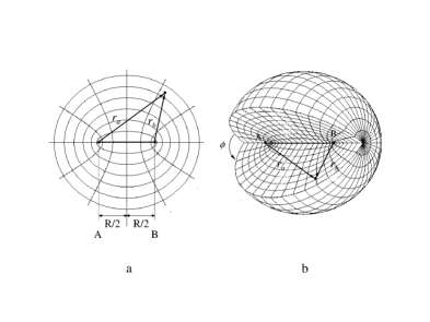
Figure 9: (a) Elliptical coordinates $(\lambda,\mu)$. (b) Prolate spheroidal coordinates $(\lambda,\mu,\phi)$ with $\lambda=(r_{a}+r_{b})/R$ and $\mu=(r_{a}-r_{b})/R$. The range of coordinates is $1\leq\lambda\leq\infty$, $-1\leq\mu\leq 1$ and $0\leq\phi\leq 2\pi$.

In Appendix A we show how to separate the variables through the use of the ellipsoidal (or, prolate spheroidal) coordinates (see Fig. 9)

$$x=\frac{R}{2}\sqrt{(\lambda^{2}-1)(1-\mu^{2})}\ \cos\phi,\quad y=\frac{R}{2}\sqrt{(\lambda^{2}-1)(1-\mu^{2})}\ \sin\phi,\quad z=\frac{R}{2}\lambda\mu.$$ (IV.14)

In such coordinates the wave function can be written as

$$\Psi=\Lambda(\lambda)M(\mu)e^{im\phi}.$$ (IV.15)

Separation of variables yields

$$\frac{d}{d\lambda}\left\{(\lambda^{2}-1)\frac{d\Lambda}{d\lambda}\right\}+\left\{A+2R_{1}\lambda-p^{2}\lambda^{2}-\frac{m^{2}}{\lambda^{2}-1}\right\}\Lambda =0, \quad R_{1} \equiv\frac{R(Z_{a}+Z_{b})}{2},\ \lambda\geq 1;$$ (IV.16)

$$\frac{d}{d\mu}\left\{(1-\mu^{2})\frac{dM}{d\mu}\right\}+\left\{-A-2R_{2}\mu+p^{2}\mu^{2}-\frac{m^{2}}{1-\mu^{2}}\right\}M =0, \quad R_{2} \equiv\frac{R(Z_{a}-Z_{b})}{2},\ |\mu|\leq 1.$$ (IV.17)

Note that $A$ and $p$ are unknown and must be solved from (IV.16) and (IV.17) as eigenvalues of the coupled system. Once $A$ and $p$ are solved, then $E$ can be obtained from (A.8).

In the next two subsections, we address the issues of solving (IV.16) and (IV.17), respectively.

IV.2.1 Solution of the $\boldsymbol{\Lambda}$-equation (IV.16)

To solve (IV.16), it is important to understand the asymptotics of the solution. Rewrite (IV.16) as

$$(\lambda^{2}-1)\Lambda^{\prime\prime}(\lambda)+2\lambda\Lambda^{\prime}(\lambda)+\left(A+2R_{1}\lambda-p^{2}\lambda^{2}-\frac{m^{2}}{\lambda^{2}-1}\right)\Lambda(\lambda)=0.$$ (IV.18)

First, consider the case $\lambda\gg 1$; we have

$$0 =\Lambda^{\prime\prime}(\lambda)+\frac{2\lambda}{\lambda^{2}-1}\Lambda^{\prime}(\lambda)+\left[\frac{A+2R_{1}\lambda}{\lambda^{2}-1}-p^{2}\frac{\lambda^{2}}{\lambda^{2}-1}-\frac{m^{2}}{(\lambda^{2}-1)^{2}}\right]\Lambda(\lambda)$$ (IV.19)

$$\approx\Lambda^{\prime\prime}(\lambda)-p^{2}\Lambda(\lambda),\quad\text{for}\quad\lambda\gg 1.$$

This gives

$$\Lambda(\lambda)\approx a_{1}e^{-p\lambda}+a_{2}e^{p\lambda},\text{ for }\lambda\gg 1,\text{ where }p>0.$$ (IV.20)

But the term $a_{2}e^{p\lambda}$ has exponential growth for large $\lambda$, which is physically inadmissible and must be discarded. Thus

$$\Lambda(\lambda)\approx a_{1}e^{-p\lambda},\quad\text{for}\quad\lambda\gg 1.$$ (IV.21)

A finer estimate than (IV.21) can be stated as follows

$$\Lambda(\lambda)=a_{0}e^{-p\lambda}\lambda^{\beta}\sum^{\infty}_{j=0}\frac{c_{j}}{\lambda^{j}}\qquad(\lambda\gg 1)$$ (IV.22)

where $\beta\equiv R_{1}/p-1$, $c_{0}=1$, $c_{1}=(p^{2}-\beta^{2}-2\beta)/(2R_{1}-2p\beta-p)$, and $a_{0}$ is an arbitrary constant. Proof is given in Appendix B.

Next, we consider the case $\lambda>1$ but $\lambda\approx 1$. In such a limit we have (see Appendix C)

$$\Lambda(\lambda)\approx(\lambda-1)^{\frac{|m|}{2}}\sum^{\infty}_{k=0}c_{k}(\lambda-1)^{k}.$$ (IV.23)

Our results in (IV.21) and (IV.23) suggest that the form

$$\Lambda(\lambda)=e^{-p\lambda}(\lambda-1)^{\frac{|m|}{2}}\lambda^{\beta}f(\lambda),\qquad\text{for some function }f(\lambda)$$ (IV.24)

would contain the right asymptotics for both $\lambda\gg 1$ and $\lambda\approx 1$. Here, obviously, $f(\lambda)$ must satisfy

$$f(1)\neq 0,\qquad\lim_{\lambda\to\infty}|f(\lambda)|\leq C,\text{ for some constant }C>0.$$ (IV.25)

Actually, in the literature (baber ; jaffe ; bates ), two improved or variant forms of the substitution of (IV.24) are found to be most useful:
(i)  (Jaffé’s solution jaffe )

$$\Lambda(\lambda)=e^{-p\lambda}(\lambda^{2}-1)^{\frac{|m|}{2}}(\lambda+1)^{\sigma}\sum_{n=0}^{\infty}g_{n}\left(\frac{\lambda-1}{\lambda+1}\right)^{n},\qquad\left(\sigma\equiv\frac{R_{1}}{p}-|m|-1\right).$$ (IV.26)

This leads to a 3-term recurrence relation

$$\alpha_{n}g_{n-1}-\beta_{n}g_{n}+\gamma_{n}g_{n+1}=0;\qquad n=0,1,2,\ldots;\quad g_{-1}\equiv 0,$$ (IV.27)

where

$$\left.\begin{array}[]{ll}\alpha_{n}=(n-1-\sigma)(n-1-\sigma-m),&\\ \beta_{n}=2n^{2}+(4p-2\sigma)n-A+p^{2}-2p\sigma-(m+1)(m+\sigma),&\\ \gamma_{n}=(n+1)(n+m+1),&\end{array}\right\}$$ (IV.28)

and, consequently, the continued fraction

$$\frac{\beta_{0}}{\gamma_{0}}=\frac{\alpha_{1}}{\beta_{1}-\dfrac{\gamma_{1}\alpha_{2}}{\beta_{2}-\dfrac{\gamma_{2}\alpha_{3}}{\beta_{3}-\ldots}}}$$ (IV.29)

for $A$ and $p$.

(ii) (Hylleraas’ solution hylleraas )

$$\Lambda(\lambda)=e^{-p(\lambda-1)}(\lambda^{2}-1)^{\frac{|m|}{2}}\sum_{n=0}^{\infty}\frac{c_{n}}{(m+n)!}L_{m+n}^{m}(x),\qquad x\equiv 2p(\lambda-1),$$ (IV.30)

where $L_{m+n}^{m}$ is the associated Laguerre polynomial and $c_{n}$ satisfy the 3-term recurrence relation

$$\alpha_{n}c_{n-1}-\beta_{n}c_{n}+\gamma_{n}c_{n+1}=0,\qquad n=0,1,2,\ldots;\quad c_{-1}\equiv 0,$$ (IV.31)

where

$$\left.\begin{array}[]{l}\alpha_{n}=(n-m)(n-m-1-\sigma),\\ \beta_{n}=2(n-m)^{2}+2(n-m)(2p-\sigma)-[A-p^{2}+2p\sigma+(m+1)(m+\sigma)],\\ \gamma_{n}=(n+1)(n-2m-\sigma),\end{array}\right\}$$ (IV.32)

and the same form of continued fractions (IV.29).

IV.2.2 Solution of the $\boldsymbol{M}$-equation (IV.17)

Equation (IV.17) has close resemblance in form with (IV.16) and, thus, it can almost be expected that the way to solve (IV.16) will be similar to that of (IV.16).

First, we make the following substitution

$$M(\mu)=e^{\pm p\mu}\widetilde{M}(\mu),\qquad-1\leq\mu\leq 1,$$ (IV.33)

in order to eliminate the $p^{2}\mu^{2}$ term in (IV.17). We obtain

$$[(1-\mu^{2})\widetilde{M}^{\prime}]^{\prime}\pm 2p(1-\mu^{2})\widetilde{M}^{\prime}+\left[(-2R_{2}\mp 2p)\mu+(p^{2}-A)-\frac{m^{2}}{1-\mu^{2}}\right]\widetilde{M}=0.$$ (IV.34)

To simplify notation, let us just consider the case $M(\mu)=e^{-p\mu}\widetilde{M}(\mu)$, but note that for $M=e^{p\mu}\widetilde{M}(\mu)$, we need only make the changes of $p\to-p$ in (IV.37) below. Write

$$M(\mu)=e^{-p\mu}\sum_{k=0}^{\infty}f_{k}P_{m+k}^{m}(\mu),$$ (IV.35)

where $P_{n}^{m}(\mu)$ are the associated Legendre polynomials, and substitute (IV.35) into (IV.17). We obtain a 3-term recurrence relation

$$\alpha_{n}f_{n-1}-\beta_{n}f_{n}+\gamma_{n}f_{n+1}=0;\qquad n=0,1,2,\ldots;f_{-1}\equiv 0,$$ (IV.36)

where

$$\left.\begin{array}[]{ll}\alpha_{n}=\dfrac{1}{2(m+n)-1}[-2nR_{2}+2pn(m+n)],&\\ \vskip 3.0pt plus 1.0pt minus 1.0pt\cr\beta_{n}=A-p^{2}+(m+n)(m+n+1),&\\ \vskip 3.0pt plus 1.0pt minus 1.0pt\cr\gamma_{n}=\dfrac{2m+n+1}{2(m+n)+3}\{-2R_{2}-2p(m+n+1)\},&\end{array}\right\}$$ (IV.37)

and, consequently, again the continued fractions of the same form as (IV.29). The continued fractions obtained here should be coupled with the continued fraction (IV.29) for the variable $\mu$ to solve $A$ and $p$.

In the homonuclear case, $R_{2}=R(Z_{a}-Z_{b})/2=0$, equation (IV.17) reduces to

$$[(1-\mu^{2})M^{\prime}]^{\prime}+\left(-A+p^{2}\mu^{2}-\frac{m^{2}}{1-\mu^{2}}\right)M=0.$$

In this case, several different optional representations of $M$ can be used:

$$\begin{array}[]{lll}\text{(a)}&M(\mu)=(1-\mu^{2})^{\frac{|m|}{2}}\sum\limits^{\infty}_{k=0}c_{k}\mu^{2k},{}{}{}{}{}{}{}{}{}{}{}{}&M(\mu)=(1-\mu^{2})^{\frac{|m|}{2}}\sum\limits^{\infty}_{k=0}c_{k}\mu^{2k+1};\end{array}$$ (IV.39)

$$\begin{array}[]{lll}\text{(b)}&M(\mu)=(1-\mu^{2})^{\frac{|m|}{2}}\sum\limits^{\infty}_{k=0}c_{k}P^{m}_{m+2k}(\mu),{}{}{}&M(\mu)=(1-\mu^{2})^{\frac{|m|}{2}}\sum\limits^{\infty}_{k=0}c_{k}P^{m}_{m+2k+1}(\mu);\end{array}$$ (IV.41)

$$\begin{array}[]{lll}\text{(c)}&M(\mu)=e^{\pm p\mu}(1-\mu^{2})^{\frac{|m|}{2}}\sum\limits^{\infty}_{k=0}c_{k}(1\mp\mu)^{k}.&\phantom{M(\mu=(1-\mu^{2})^{\frac{|m|}{2}}\sum\limits^{\infty}_{k=0}}\end{array}$$ (IV.43)

In Appendix D we discuss expansions of solution near $\boldsymbol{\lambda\approx 1}$ and $\boldsymbol{\lambda\gg 1}$ and their connection with the James–Coolidge trial wave functions.

As a conclusion of this section, we note that the eigenstates of the hydrogen atom given in the preceding subsection can also be easily represented in terms of the prolate spheroidal coordinates. We let the nucleus of H (i.e., a proton) sit at location $a$ where $(0,0,-R/2)$ with $Z_{a}=1$ while at location $b$ where $(0,0,R/2)$ we let $Z_{b}=0$. Thus, the hydrogen atom satisfies Eq. (IV.13) in the form

$$H\psi=\left(-\frac{1}{2}\nabla^{2}-\frac{1}{r_{a}}\right)\psi=E\psi.$$ (IV.44)

Now, in terms of the prolate spheroidal coordinates (A.3) in Appendix A, and

$$\psi(\lambda,\mu,\phi)=\Lambda(\lambda)M(\mu)\Phi(\phi),\text{ where }\Phi(\phi)=e^{im\phi}$$ (IV.45)

in the form of separated variables, we have

$$-\frac{1}{2}\frac{4}{R^{2}(\lambda^{2}-\mu^{2})}\left\{\frac{\partial}{\partial\lambda}\left[(\lambda^{2}-1)\frac{\partial}{\partial\lambda}\Lambda\right]M+\frac{\partial}{\partial\mu}\left[(1-\mu^{2})\frac{\partial}{\partial\mu}M\right]\Lambda-\frac{(\lambda^{2}-\mu^{2})m^{2}}{(\lambda^{2}-1)(1-\mu^{2})}M\Lambda\right\}$$

$$\qquad-\frac{2}{R}\frac{1}{\lambda-\mu}M\Lambda=EM\Lambda,$$

which has two fewer terms than (A.6) does as now $Z_{b}=0$. Set $p^{2}=-R^{2}E/2$, we again have (IV.16) and (IV.17) except that now $R_{1}=R_{2}=R/2$ therein. The rest of the procedures follows in the same way with some minor adjustments as noted above.

The above discussion also leads to a sequence of identities between (IV.6) and (IV.45), as

$$\psi^{(1)}(x,y,z)=\psi^{(2)}\left(x,y,z+\frac{R}{2}\right),$$

where $\psi^{(1)}(x,y,z)$ is an eigenstate of the hydrogen atom obtained from (IV.2) but expressed in terms of the Cartesian coordinates $(x,y,z)$ while $\psi^{(2)}(x,y,z)$ is that for the solution of (IV.44).

IV.3 The many-centered, one-electron problem

When $N_{e}=1$ and $N\geq 3$ in (IV.1), we have a molecular ion with three or more nuclei sharing one electron. A simple example is a $CO_{2}$-like structure, with $N=3$. For such a problem, separable closed-form solutions are extremely difficult to come by from the traditional line of attack. However, we want to describe an elegant analysis by T. Shibuya and C.E. Wulfman SW (see also the book by B.R. Judd Judd ) which works in momentum space and expand electron’s eigenfunction as a linear combination of 4-dimensional spherical harmonics. This analysis may offer useful help to the modeling and computation of complex molecules after proper numerical realization.

The model equation reads

$$\left(-\frac{1}{2}\nabla^{2}-\sum_{j=1}^{N}\frac{Z_{j}}{|\boldsymbol{r}-\boldsymbol{R}_{j}|}\right)\psi(\boldsymbol{r})=E\psi(\boldsymbol{r}),\qquad\boldsymbol{r}=(x,y,z)\in{\mathbb{R}}^{3},$$ (IV.46)

where ${\bf R}_{j}$ are positions of the nuclei.

Appendix E shows how to reduce the problem to a matrix form. Here we provide the answer for the energy; it is determined from the solution of the eigenvalue equation

$$\boldsymbol{P}{\bf c}=\sqrt{-2E}{\bf c},$$ (IV.47)

where ${\bf c}$ is an infinite dimensional vector, $\boldsymbol{P}$ is an infinite matrix with entries

$$P_{n^{\prime}\ell^{\prime}m^{\prime}}^{n\ell m}=\sum_{j}Z_{j}\sum_{n^{\prime\prime}\ell^{\prime\prime}m^{\prime\prime}}\left[S_{n^{\prime\prime}\ell^{\prime\prime}m^{\prime\prime}}^{n^{\prime}\ell^{\prime}m^{\prime}}({\bf R}_{j})\right]^{*}\frac{1}{n}S_{n^{\prime\prime}\ell^{\prime\prime}m^{\prime\prime}}^{n\ell m}({\bf R}_{j}),$$ (IV.48)

$$n,n^{\prime},n^{\prime\prime}=1,2,3,\ldots;\ell,\ell^{\prime},\ell^{\prime\prime}=0,1,2,\ldots;m,m^{\prime},m^{\prime\prime}=-\ell,-\ell+1,\ldots,-1,0,1,\ldots,\ell-1,\ell;$$

the matrix $S$ is given by an integral over 4-dimensional unit hypersphere S₃ with the surface element $d\Omega=\sin^{2}\chi\sin\theta d\chi d\theta d\phi$,

$$S_{n^{\prime}\ell^{\prime}m^{\prime}}^{n\ell m}({\bf R}_{j})=\int_{S_{3}}\exp(i{\bf R}_{j}\cdot{\bf p})Y_{n\ell m}(\Omega)Y_{n^{\prime}\ell^{\prime}m^{\prime}}(\Omega)d\Omega\text{,}$$ (IV.49)

$Y_{n\ell m}(\Omega)$ is a product of the spherical function $Y_{\ell m}(\theta,\phi)$ and the associated Gegenbauer function $C_{n}^{\ell}(\chi)$

$$Y_{n\ell m}(\Omega)=(-i)^{\ell}C_{n}^{\ell}(\chi)Y_{\ell m}(\theta,\phi).$$

The 3-dimensional vector ${\bf p}$ in Eq. (IV.49) has components

$$p_{x}=p\sin\theta\cos\phi,\quad p_{y}=p\sin\theta\sin\phi,\quad p_{z}=p\cos\theta,\quad\text{where}\quad p=\sqrt{-2E}\tan(\chi/2)\text{.}$$

In practice, the infinite matrix $\boldsymbol{P}$ in (IV.48) is truncated to a finite size square matrix according to the quantum numbers $(n\ell m)$ for which the restriction $n\leq n_{0}$ is specified for some positive integer $n_{0}$.

In the derivation, if we restrict $N=1$, $Z_{1}=1$ and set $\boldsymbol{R}_{1}=0$, then the matrix $\boldsymbol{P}$ is diagonal and we recover the hydrogen atom as derived in Subsection IV.1. Obviously, if $N=2$, by setting $\boldsymbol{R}_{1}=(0,0,-R/2)$ and $\boldsymbol{R}_{2}=(0,0,R/2)$, we should also be able to recover those H${}_{2}^{+}$-like solutions given in Subsection IV.B.

The 1-electron one-centered or two-centered orbitals derived in Subsection IV.A and IV.B will be utilized frequently in the rest of the paper. At the present time, there is very limited knowledge about the 1-electron many-centered orbitals as discussed in Subsection IV.C. There seems to be abundant space for their exploitation in molecular modeling and computation in the future.

V Two electron molecules: cusp conditions and correlation functions

V.1 The cusp conditions

In the study of any linear partial differential equations with singular coefficients, it is well known to the theorists that solutions will have important peculiar behavior at and near the locations of the singularities. We have first encountered such singularities in Subsection III.3.1. Here we give singularities of the Coulomb type a more systematic treatment. The critical mathematical analysis was first made by Kato Ka in the form of cusp conditions for the Born–Oppenheimer separation.

Consider the following slightly more general form of the Schrödinger equation for a 2-particle system

$$(\hat{H}-E)\psi=0,$$ (V.1)

where

$$\hat{H}=-\frac{1}{2m_{1}}\nabla_{1}^{2}-\frac{1}{2m_{2}}\nabla_{2}^{2}-\frac{Z_{a}}{r_{1a}}-\frac{Z_{b}}{r_{1b}}-\frac{Z_{a}}{r_{2a}}-\frac{Z_{b}}{r_{2b}}+\frac{q_{1}q_{2}}{r_{12}}+\frac{Z_{a}Z_{b}}{R}.$$ (V.2)

The operator $\hat{H}$ has five sets of singularities, at

$$r_{1a}=0,\quad r_{1b}=0,\quad r_{2a}=0,\quad r_{2b}=0\quad\text{and}\quad r_{12}=0.$$ (V.3)

It has been proved by Kato Ka that the wave function $\psi$ is Hölder continuous, with bounded first order partial derivatives. However, these first order partial derivatives $\partial\psi/\partial x_{i}$, etc., $i=1,2,\ldots,6$, are discontinuous at (V.3). In the terminology of the mathematical theory of partial differential equations, (V.2) is said to have a nontrivial solution in the Sobolev space $H^{1}({\mathbb{R}}^{6})$.

We now discuss the cusp conditions at these singularities. What is a cusp condition? It can be simply explained in the following paragraph. Let us elucidate it for the two particle Hamiltonian (V.2); for a multi-particle Hamiltonian the idea is the same.

In order for the wave function $\psi$ to satisfy the eigenvalue problem (V.1) at the singularities (V.3), the kinetic energy operators $-\nabla_{1}^{2}/2m_{1}$ and $-\nabla_{2}^{2}/2m_{2}$, after acting on $\psi$, must produce terms that exactly cancel those singularity terms in the potential in order to give us back just a constant $E$ times $\psi$, because the wave function $\psi$ is bounded everywhere in space, including the points where the nuclei are located, without exception. One can see that, if the cusp conditions are not satisfied, then there is some unboundedness at the singularities (V.3) which can affect the accuracy in numerical computations. Conversely, if the cusp conditions are satisfied, this normally improves the numerical accuracy.

In case we don’t know the exact eigenstate, but only a certain trial wave function, say $\phi$, then $(\hat{H}-E)\phi=0$ will not be satisfied in general. Rather, we have

$$(\hat{H}-E)\phi(\boldsymbol{r}_{1},\boldsymbol{r}_{2})=f(\boldsymbol{r}_{1},\boldsymbol{r}_{2})$$

for some function $f$ depending on the spatial variables $\boldsymbol{r}_{1}$ and $\boldsymbol{r}_{2}$. However, we can insist on choosing parameters in $\phi$ such that the residual $f(\boldsymbol{r}_{1},\boldsymbol{r}_{2})$ is a bounded function everywhere; in particular, $f(\boldsymbol{r}_{1},\boldsymbol{r}_{2})$ cannot contain any singularity at (V.3). We say that the trial wave function $\phi$ satisfies

• the electron-nucleus cusp condition at $a$ (resp. $b$) if $f$ is not singular at $a$ (resp. $b$);

• the interelectronic (or electron-electron) cusp condition if $f$ is not singular when $r_{12}=0$.

For example, in the simple case of a hydrogen atom,

$$\hat{H}=-\frac{1}{2}\nabla^{2}-\frac{1}{r},$$

let $\phi(\boldsymbol{r})=Ce^{-\alpha r}$ be a trial wave function. Then for any $E$,

$$(\hat{H}-E)\phi=C\left\{\frac{(\alpha-1)e^{-\alpha r}}{r}-(E+\alpha^{2}/2)e^{-\alpha r}\right\}.$$

The singularity $1/r$ can be eliminated only by choosing $\alpha=1$. This is the cusp condition, which actually forces $\phi$ to be the ground state (with $E=-1/2$). The profile of $\phi$, as shown in Fig. 10 illustrates the appearance of a cusp at the origin.

Figure 10: A 1-dimensional cross section of $\boldsymbol{\phi(r)=e^{-r}}$ showing a cusp.

In Appendix F we derive the cusp conditions for the two particle electron wave function $\psi$ of (V.1):

$$\left.\frac{\partial\psi}{\partial r_{1a}}\right|_{r_{1a}=0}=-m_{1}Z_{a}\psi(r_{1a}=0),\quad\left.\frac{\partial\psi}{\partial r_{1b}}\right|_{r_{1b}=0}=-m_{1}Z_{b}\psi(r_{1b}=0),$$ (V.4)

$$\left.\frac{\partial\psi}{\partial r_{2a}}\right|_{r_{2a}=0}=-m_{2}Z_{a}\psi(r_{2a}=0),\quad\left.\frac{\partial\psi}{\partial r_{2b}}\right|_{r_{2b}=0}=-m_{2}Z_{b}\psi(r_{2b}=0),$$ (V.5)

$$\left.\frac{\partial\psi}{\partial r_{12}}\right|_{r_{12}=0}=\frac{m_{1}m_{2}}{m_{1}+m_{2}}q_{1}q_{2}\psi(r_{12}=0).$$ (V.6)

Eqs. (V.4), (V.5) are the electron-nucleus cusp condition, while Eq. (V.6) is the interelectronic condition.

In forming trial wave functions from one-centered or two-centered orbitals for a homonuclear diatomic molecule a commonly used wave function is

$$\psi(\boldsymbol{r}_{1},\boldsymbol{r}_{2})=\phi(\boldsymbol{r}_{1})\phi(\boldsymbol{r}_{2})f(r_{12}),\quad f(r_{12})=1+\frac{1}{2}r_{12},\qquad\text{(cf.\ \eqref{I.17})}$$ (V.7)

where $\phi(\boldsymbol{r}_{i})$, $i=1,2$, is an orbital for the molecular ion. In Appendix F we show that (V.7) satisfies the interelectronic cusp condition. If, however, $\phi_{1}\neq\phi_{2}$, then the trial wave function

$$\psi(\boldsymbol{r}_{1},\boldsymbol{r}_{2})=\phi_{1}(\boldsymbol{r}_{1})\phi_{2}(\boldsymbol{r}_{2})\left(1+\frac{1}{2}r_{12}\right)$$

satisfies the interelectronic cusp condition if and only if

$$\phi_{2}(\boldsymbol{r})\nabla\phi_{1}(\boldsymbol{r})-\phi_{1}(\boldsymbol{r})\nabla\phi_{2}(\boldsymbol{r})=\boldsymbol{0}.$$

The actual verifications of cusp conditions for specifically given examples of trial wave functions in the cases of one-centered orbitals or their products are not difficult. But such work is nontrivial when the trial wave functions are expressed in terms of prolate spheroidal coordinates. In Appendix H we illustrate through concrete examples how to carry out this task.

V.2 Various forms of the correlation function $\boldsymbol{f(r_{12})}$

We have learned the importance of the interelectronic cusp condition in Section V.1. But there are, in addition, three important constructs that are crucial for diatomic calculations: orbitals, configurations and electronic correlation. In this section, we compile a list of often cited correlation functions $f$ which help the satisfaction of the interelectronic cusp conditions in the context of Eq. (V.6). The study of the other two, i.e., orbitals and configurations, will be addressed in the next section.

(1) $\displaystyle\boldsymbol{f(r_{12})=1+\frac{1}{2}r_{12}}$.

This is the simplest possible interelectronic configuration function. The specific form is due to the correlation cusp condition only. We derive it as follows (see Patil, Tang & Toennies PTT ). Consider two charged particles which are described by the Schrödinger equation

$$\left(-\frac{1}{2m_{1}}\nabla_{1}^{2}-\frac{1}{2m_{2}}\nabla_{2}^{2}+\frac{q_{1}q_{2}}{r_{12}}\right)\psi=\epsilon\psi.$$ (V.8)

First, transform the above equation to the center-of-mass coordinates (cf. Appendix G)

$$\left(-\frac{1}{2M}\nabla_{S}^{2}-\frac{1}{2\mu}\nabla_{r_{12}}^{2}+\frac{q_{1}q_{2}}{r_{12}}\right)\psi=\epsilon\psi,$$ (V.9)

where

$$M=m_{1}+m_{2},\quad\mu=\frac{m_{1}m_{2}}{m_{1}+m_{2}},\quad\boldsymbol{S}=\frac{m_{1}\boldsymbol{r}_{1}+m_{2}\boldsymbol{r}_{2}}{m_{1}+m_{2}},\qquad\boldsymbol{r}_{12}=\boldsymbol{r}_{1}-\boldsymbol{r}_{2}.$$ (V.10)

In the ground state $\psi$ is independent of $\boldsymbol{S}$. Near the singularity point $r_{12}=0$, the wave function $\psi$ has a local representation as a power series

$$\psi=C_{0}+C_{1}r_{12}+{\mathcal{O}}(r_{12}^{2}).$$ (V.11)

Substituting (V.11) into (V.9) and using $\nabla_{r}^{2}=\frac{1}{r^{2}}\frac{\partial}{\partial r}\left(r^{2}\frac{\partial}{\partial r}\right)$ we obtain

$$\frac{1}{r_{12}}\left(-\frac{C_{1}}{\mu}+q_{1}q_{2}C_{0}\right)+\left(-\frac{3C_{2}}{\mu}+C_{1}q_{1}q_{2}\right)+\cdots=\epsilon(C_{0}+C_{1}r_{12}+{\mathcal{O}}(r^{2}_{12}))$$ (V.12)

The above mandates that the coefficient of $1/r_{12}$ must vanish, that is

$$C_{1}=\mu q_{1}q_{2}C_{0},$$

which for $\mu=1/2$ (i.e., $m_{1}=m_{2}$), and $q_{1}=q_{2}=1$, yields

$$C_{1}=\frac{1}{2}C_{0}.$$

This gives us the small $r_{12}$ behavior

$$\psi=C_{0}\left(1+\frac{1}{2}r_{12}\right),$$ (V.13)

where we have dropped all the ${\mathcal{O}}(r_{12}^{2})$ terms. The asymptotic expression (V.13) motivates the choice of $f(r_{12})$ in such particular form.

This simple $f(r_{12})$ captures short distance interelectronic interaction very well. It offers elegant representations of molecular orbitals and great facility to computation. Nevertheless, its asymptotic behavior of linear growth for large $r_{12}$ is not physically correct.

When we write molecular orbitals as

$$\psi(\boldsymbol{r}_{1},\boldsymbol{r}_{2},r_{12})=\phi(\boldsymbol{r}_{1},\boldsymbol{r}_{2})f(r_{12}),$$

if the function $\phi(\boldsymbol{r}_{1},\boldsymbol{r}_{2})$ is already quite small in the region where $r_{12}$ becomes large compared to 1, then this simple $f(r_{12})=1+\frac{1}{2}r_{12}$ can work quite well (Kleinekathöfer et al. (K, , pp. 2841–2842)).

(2)  $\displaystyle\boldsymbol{f(r_{12})=1+\frac{r_{12}}{2}e^{-r_{12}/d},\quad(d>0)}$

This function was proposed by Hirschfelder Hir where $d$ is a variational parameter. Its profiles is shown in Fig. 11. It satisfies the cusp condition near $r_{12}=0$. This function was used by Siebbles, Marshall and Le Sech SML . Nevertheless, Le Sech et al. SML ; Sech96 reported that in performing variational calculations by writing $f(r_{12})=1+\frac{r_{12}}{2}e^{-\alpha r_{12}}$, they found that $\alpha$ is computed to be very close to 0 for small and intermediate $R$. That is, it virtually degenerates into $f(r_{12})=1+\frac{1}{2}r_{12}$. However, at large $R$ one should use $\alpha\neq 0$ in order to obtain the correct dissociation limit.

Figure 11: Graph of $\boldsymbol{f(r_{12})=1+\frac{r_{12}}{2}e^{-r_{12}/d}}$, where the maximum happens at $\boldsymbol{r_{12}=d}$.

¿From physical considerations, there is no reason to believe why $f(r_{12})$ should have a local maximum as shown in Fig. 11. Even though the choice of this $f(r_{12})$ seems satisfactory asymptotically for both $r_{12}$ small and large, it may not be satisfactory for medium values of $r_{12}$.

(3) $\displaystyle\boldsymbol{f(r_{12})=1-\frac{1}{1+2\lambda}e^{-\lambda r_{12}},(\lambda>0)}$

This correlation function is partly motivated by Hirschfelder’s work Hir , and partly by Hylleraas study of the helium atom hylleraas . It was introduced by Kleinekathöfer et al. K .

At small $r_{12}$ we have the expansion

$$f(r_{12})=\frac{2\lambda}{1+2\lambda}\left(1+\frac{1}{2}r_{12}-\frac{\lambda}{4}r_{12}^{2}\pm\cdots\right).$$

Therefore the cusp condition is satisfied for any $\lambda>0$. This $\lambda$ can be either used as a variational parameter, or be determined from a given Hamiltonian. For example, for a helium-like 2-electron atom with nuclear charge $Z$, using a perturbation argument, Kleinekathöfer et al. K analyzed that the best value for $\lambda$ is

$$\lambda=\frac{5}{12}Z-\frac{1}{3}.$$

This $f(r_{12})$ has a monotone profile and correct asymptotics for both $r_{12}$ small and large. See Fig. 12.

Figure 12: Graph of $\boldsymbol{f(r_{12})=1-\frac{1}{1+2\lambda}e^{-\lambda r_{12}}}$.

(4) $\displaystyle\boldsymbol{f(r_{12})=e^{\frac{1}{2}r_{12}}}$.

This $f(r_{12})$ satisfies the correlation-wave equation

$$\left(-\frac{1}{2}\nabla_{1}^{2}-\frac{1}{2}\nabla_{2}^{2}+\frac{1}{r_{12}}\right)e^{\frac{1}{2}r_{12}}=-\frac{1}{4}e^{\frac{1}{2}r_{12}}$$

with a negative energy $-1/4$. For small $r_{12}$, its expansion is

$$e^{\frac{1}{2}r_{12}}=1+\frac{1}{2}r_{12}+{\mathcal{O}}(r_{12}^{2}).$$

Therefore, it satisfies the correlation-cusp condition and its asymptotics for small $r_{12}$ is good. However, this $f(r_{12})$ has exponential growth for large $r_{12}$ and is thus physically incorrect.

(5) $\displaystyle\boldsymbol{f(r,r_{12})=\frac{\sinh(tr)}{tr}\cdot\frac{F_{0}(\frac{1}{2k},kr_{12})}{r_{12}}}$

where $F_{j}(\eta,\rho)$ is the Coulomb wave function regular at the origin, $j$ is an integer, $t,k$ are separation of variables constants and $r=|{\bf r}_{1}+{\bf r}_{2}|$.

This is perhaps the most complex form of the correlation function in the literature, given by Aubert–Frécon and Le Sech A-FL . It comes from solving

$$\left\{-\frac{1}{2}\nabla_{1}^{2}-\frac{1}{2}\nabla_{2}^{2}+\frac{1}{r_{12}}\right\}f=\epsilon f.$$ (V.14)

Rewrite the above in center-of-mass coordinates:

$$\left(-\frac{1}{4}\nabla_{S}^{2}-\nabla_{r_{12}}^{2}+\frac{1}{r_{12}}\right)f=\epsilon f.$$ (V.15)

Assume that $f$ depends only on $r,r_{12}$ and $\gamma$, where $\gamma$ is the angle between $\boldsymbol{S}$ and $\boldsymbol{r}_{12}$ (see Fig. 13).

Figure 13: The variables $\boldsymbol{r,r_{12}}$ and angle $\boldsymbol{\gamma}$ in the center-of-mass coordinates.

Then equation (V.15) can be written as

$$-\frac{1}{r^{2}_{12}}\frac{\partial}{\partial r_{12}}\left(r^{2}_{12}\frac{\partial f}{\partial r_{12}}\right)-\frac{1}{r^{2}}\frac{\partial}{\partial r}\left(r^{2}\frac{\partial f}{\partial r}\right)-\left[\frac{1}{r^{2}_{12}}\frac{\partial}{\partial q}(1-q^{2})\frac{\partial}{\partial q}f\right]$$

$$\quad-\left[\frac{1}{r^{2}}\frac{\partial}{\partial q}(1-q^{2})\frac{\partial f}{\partial q}\right]+\frac{1}{r_{12}}f=\epsilon f,\qquad q\equiv\cos\gamma.$$ (V.16)

Equation (V.16) can be separated by writing

$$f=P_{j}(q)g^{j}(r)u^{j}(r_{12}),$$

where

$$\frac{\partial}{\partial q}(1-q^{2})\frac{\partial P_{j}}{\partial q}=-j(j+1)P_{j},$$ (V.17)

$P_{j}$ is the Legendre polynomial of degree $j$ and $g^{j}(r)$ and $u^{j}(r_{12})$ satisfy, respectively,

$$\left\{\frac{d^{2}}{dr^{2}}+\frac{2}{r}\frac{d}{dr}-\frac{j(j+1)}{r^{2}}+\epsilon_{g}\right\}g^{j}(r)=0,$$ (V.18)

$$\left\{\frac{d^{2}}{dr^{2}_{12}}+\frac{2}{r_{12}}\frac{d}{dr_{12}}-\frac{j(j+1)}{r^{2}_{12}}-\frac{1}{r_{12}}+\epsilon_{u}\right\}u^{j}(r_{12})=0,$$ (V.19)

with

$$\epsilon=\epsilon_{g}+\epsilon_{u}.$$

Take

$$\epsilon_{g}=-t^{2},\quad\epsilon_{u}=k^{2},\quad j=0.$$ (V.20)

Then

$$P_{0}(q)=1,\quad g^{0}_{t}(r)=\frac{\sinh(tr)}{tr},\quad u^{0}_{k}=\frac{F_{0}(\frac{1}{2k},kr_{12})}{r_{12}},$$

where the function $F_{0}(\eta,\rho)$ belongs to the class of regular Coulomb wave function $F_{L}(\eta,\rho)$, satisfying

$$\frac{d^{2}}{d\rho^{2}}F_{L}(\eta,\rho)+\left[1-\frac{2\eta}{\rho}-\frac{L(L+1)}{\rho^{2}}\right]F_{L}(\eta,\rho)=0$$

for the two parameters $\eta$ and $L$.

Note that $t$ and $k$ in (V.20) can be used as variational parameters. For small $r_{12}$,

$$F_{0}\left(\frac{1}{2k},kr_{12}\right)=C\cdot kr_{12}\left[1+\frac{1}{2}r_{12}+{\mathcal{O}}((kr_{12})^{2})\right]$$

and, thus,

$$u_{k}^{0}(r_{12})=\frac{F_{0}(\frac{1}{2k},kr_{12})}{r_{12}}=C\cdot k\left[1+\frac{1}{2}r_{12}+{\mathcal{O}}((kr_{12})^{2})\right]$$

satisfies the correlation-cusp condition for any given $k$.

For large $r_{12}$, the Coulomb wave function $F_{L}(\eta,\rho)$ has an asymptotic expansion

$$F_{L} =g\cos\theta_{L}+f\sin\theta_{L},$$

$$\theta_{L} \equiv\rho-\eta\ln z\rho-L\frac{\pi}{2}+\sigma_{L},$$

$$\sigma_{L} \equiv\arg\Gamma(L+1+i\eta),$$

$$f \sim\sum^{\infty}_{k=0}f_{k},\quad g\sim\sum^{\infty}_{k=0}g_{k},$$

$$f_{0} =1,\quad g_{0}=1,$$

$$f_{k+1} =a_{k}f_{k}-b_{k}g_{k},\quad g_{k+1}=a_{k}g_{k}+b_{k}f_{k},$$

$$a_{k} =\frac{(2k+1)\eta}{(2k+2)\rho},\quad b_{k}=\frac{L(L+1)-k(k+1)+\eta^{2}}{(2k+2)\rho}.$$

Thus

$$\lim_{r_{12}\to\infty}u^{0}_{k}(r_{12})=\lim_{r_{12}\to\infty}\frac{F_{0}(\frac{1}{2k},kr_{12})}{r_{12}}=0.$$

(6) $\displaystyle\boldsymbol{f(r_{12})={}_{1}F_{1}\left(-\frac{1}{2Z},2,-2Zr_{12}\right)}$

where ${}_{1}F_{1}(a;b;x)$ is the confluent hypergeometric function satisfying the differential equation

$$x\frac{d^{2}w}{dx^{2}}+(b-x)\frac{dw}{dx}-aw=0.$$ (V.21)

This $f(r_{12})$ was given by Patil, Tang and Toennies PTT for the case when the internuclear separation $R$ is large:

$$R\gg\frac{3}{Z}.$$ (V.22)

Its derivation can be motivated as follows. Consider

$$H=-\frac{1}{2}\nabla^{2}_{1}-\frac{1}{2}\nabla^{2}_{2}-\left(\frac{Z}{r_{1a}}+\frac{Z}{r_{1b}}+\frac{Z}{r_{2a}}+\frac{Z}{r_{2b}}\right)+\frac{1}{r_{12}}+\frac{Z^{2}}{R}$$ (V.23)

for an H₂-like molecule. Guillemin–Zener-type one-electron wave functions GZ suggest the molecular orbital for large $R$:

$$\Psi=(e^{-Zr_{1a}-Zr_{2b}}+e^{-Zr_{1b}-Zr_{2a}})f(r_{12}).$$ (V.24)

When $R$ is large, electron 1 is localized around $A$ and electron 2 is localized around $B$, as shown in Fig. 14.

Figure 14: For large $\boldsymbol{R}$, electron $\boldsymbol{e_{1}}$ is localized near $\boldsymbol{A}$, and electron $\boldsymbol{e_{2}}$ is localized near $\boldsymbol{B}$.

We have

$$r_{1b}\gg r_{1a},\quad r_{2a}\gg r_{2b}.$$ (V.25)

Because of (V.25), we have, from (V.24),

$$\Psi =(e^{-Zr_{1a}-Zr_{2b}}+e^{-Zr_{1b}-Zr_{2a}})f(r_{12})$$

$$\approx e^{-Zr_{1a}-Zr_{2b}}f(r_{12}).$$ (V.26)

Substituting (V.26) into $\hat{H}\psi=E\psi$, we obtain

$$-\frac{1}{2}(\nabla_{1}^{2}+\nabla_{2}^{2})f+Z(\nabla_{1}f)\cdot(\hat{\boldsymbol{r}}_{1a}+\hat{\boldsymbol{r}}_{2b})+\frac{1}{r_{12}}f={\mathcal{}}\mathcal{O}\left(\frac{1}{R}\right).$$ (V.27)

Note that Eq. (V.27) contains the effect of cross terms. For large $R$, the electron-electron correlation is most significant when the two electrons are colinear and in between the two nuclei. In this situation, either $\boldsymbol{r}_{12}$ is antiparallel to $\boldsymbol{r}_{1}-\boldsymbol{r}_{a}$, or $\boldsymbol{r}_{12}$ is parallel to $\boldsymbol{r}_{2}-\boldsymbol{r}_{b}$.

Now, using the center-of-mass coordinates and dropping all the ${\mathcal{O}}\left(1/R\right)$ terms, we obtain

$$-\left(\frac{\partial^{2}}{\partial r_{12}^{2}}+\frac{2}{r_{12}}\frac{\partial}{\partial r_{12}}\right)f+\frac{1}{r_{12}}f-2Z\frac{\partial f}{\partial r_{12}}=0.$$ (V.28)

The solution to (V.28), after setting it into the form of (V.21) is

$$f(r_{12})={}_{1}F_{1}\left(-\frac{1}{2Z},2,-2Zr_{12}\right).$$

For small $r_{12}$, the expansion is

$$f(r_{12})=1+\frac{1}{2}r_{12}-\frac{(2Z-1)}{12}r_{12}^{2}+\cdots~{}.$$

Therefore, the correlation-cusp condition is satisfied. For large $r_{12}$, the asymptotics is

$$f(r_{12})\sim C(-2Zr_{12})^{\frac{1}{2Z}}$$

(cf. Abramowitz and Stegun (AS, , p. 508, 13.5.1)).

VI Modeling of diatomic molecules

In this section, we give a survey of major existing methods for the numerical modeling of diatomic molecules. These methods provide approximations of wave functions either in explicit form through properly selected ansatzs, or in implicit form through iterations as numerical solutions of integro-partial differential equations.

The methods and ansatzs to be described below are

• The Heitler–London method;

• The Hund–Mulliken method;

• The Hartree–Fock (self-consistent) method;

• The James–Coolidge wave function;

• Two-centered orbitals;

Items (1)$\sim$(3) above historically are associated with one-centered orbitals, while (4)$\sim$(5) are based on two-centered orbitals. But this dichotomy is not inflexible. An example is a hybrid type containing both one-centered and two-centered orbitals considerd in Subsection III.C.6. We now discuss them in sequential order below. Each approach has a set of modeling parameters which can be optimized through calculus of variations. In particular, we will point out what these parameters are.

VI.1 The Heitler–London method

This method has the longest history. It was developed by Heitler and London during the 1920s soon after Heisenberg laid the quantum mechanical foundation of ferromagnetism. The method is usually called the valence-bond (or atomic orbital) method. In this method, each molecule is thought of as composed of atoms, and the electronic structure is described using atomic orbitals of these atoms.

Here we present a version of refined Heitler–London approach due to Slater Slat63 . In the method, electron spin-orbitals are taken from a determinant

$$\left|\begin{matrix}u_{1}(1)&u_{1}(2)&\cdots&u_{1}(n)\\ u_{2}(1)&u_{2}(2)&\cdots&u_{2}(n)\\ \cdots\\ u_{n}(1)&u_{n}(2)&&u_{n}(n)\end{matrix}\right|,$$ (VI.1)

which satisfy the Fermionic property of the Pauli exclusion principle. The orbitals in (VI.1) are called the Slater orbitals. Let us consider the 2-electron case, i.e., $n=2$ in (VI.1). The spin-orbital $u_{i}(j)$, $i,j=1,2$, consists of

(i)  the electron-atomic orbital part

$$a(1) =\sqrt{\frac{\alpha^{3}}{\pi}}e^{-\alpha r_{1a}}, \qquad a(2) =\sqrt{\frac{\alpha^{3}}{\pi}}e^{-\alpha r_{2a}},$$ (VI.2)

$$b(1) =\sqrt{\frac{\alpha^{3}}{\pi}}e^{-\alpha r_{1b}}, \qquad b(2) =\sqrt{\frac{\alpha^{3}}{\pi}}e^{-\alpha r_{2b}},$$ (VI.3)

where in (VI.2) and (VI.3), the atomic electron wave functions are centered at, respectively, $a$ and $b$.

(ii)  the spin part

$$\begin{matrix}\text{spin}&\alpha(1),&\alpha(2),&\alpha(j)=|s,m_{s}\rangle,&\uparrow,&\text{for }j=1,2,\\ \text{spin}&\beta(1),&\beta(2),&\beta(j)=|s,m_{s}\rangle&\downarrow,&\text{for }j=1,2.\end{matrix}$$

The linear combinations of the total spin-orbital wave function that are antisymmetric are tabulated below:

$$\begin{array}[]{|c|l|c|}\hline\cr&\lx@intercol\hfil\text{spin-orbital wave functions}\hfil\lx@intercol\vrule\lx@intercol&M_{s}\text{ (total spin)}\\ \hline\cr\text{singlet state}&[a(1)b(2)+b(1)a(2)][\alpha(1)\beta(2)-\beta(1)\alpha(2)]&0\\ \hline\cr&[a(1)b(2)-b(1)a(2)][\alpha(1)\alpha(2)]&1\\ \cline{2-3}\cr\text{triplet states}&[a(1)b(2)-b(1)a(2)][\alpha(1)\beta(2)+\beta(1)\alpha(2)]&0\\ \cline{2-3}\cr&[a(1)b(2)-b(1)a(2)][\beta(1)\beta(2)]&-1\\ \hline\cr\end{array}$$ (VI.4)

Table 1. Spin-orbital wave functions of singlet and triplet states

The singlet state has lower energy than the triplets. For example, if we aim to calculate the ground state of H₂, we use (VI.4) as the trial wave function to minimize the total energy

$$\langle\Psi|{\hat{H}}|\Psi\rangle,\text{ subject to }\langle\Psi|\Psi\rangle=1,$$ (VI.5)

where

$${\hat{H}} =-\frac{1}{2}\nabla^{2}_{1}-\frac{1}{2}\nabla^{2}_{2}-\frac{1}{r_{1a}}-\frac{1}{r_{1b}}-\frac{1}{r_{2a}}-\frac{1}{r_{2b}}+\frac{1}{r_{12}}+\frac{1}{R}$$ (VI.6)

$$\Psi ={\mathcal{N}}[a(1)b(2)+b(1)a(2)],\quad{\mathcal{N}}=\text{ a normalization factor.}$$ (VI.7)

Heisenberg, and Heitler–London’s basic point of view is that ${\hat{H}}$ in (VI.6) can be written as

$${\hat{H}}=\left(-\frac{1}{2}\nabla^{2}_{1}-\frac{1}{r_{1a}}\right)+\left(-\frac{1}{2}\nabla^{2}_{2}-\frac{1}{r_{2b}}\right)+\left(-\frac{1}{r_{1b}}-\frac{1}{r_{2a}}+\frac{1}{r_{12}}+\frac{1}{R}\right),$$

where the terms inside the third pair of parentheses above can be viewed as a “perturbation.”

Since the Heitler–London method is quite fundamental in molecular chemistry, let us give some details about the calculation of (VI.5) given (VI.6) and (VI.7).

Define

$$S \equiv\text{the overlap }\equiv\langle a(1)|b(1)\rangle=\int\limits_{{\mathbb{R}}^{3}}e^{-\alpha r_{1a}}e^{-\alpha r_{1b}}\ dx\cdot\frac{\alpha^{3}}{\pi}\qquad(dx=dx_{1}dx_{2}dx_{3})$$

$$=e^{-\alpha R}\left[1+\alpha R+\frac{(\alpha R)^{2}}{3}\right].$$

Then $\langle a(1)b(2)|a(2)b(1)\rangle=\langle a(1)|b(1)\rangle\langle b(2)|a(2)\rangle=S^{2}$, and the normalized state for the singlet or the triplets, without spin, is

$$\Psi=\frac{a(1)b(2)\pm a(2)b(1)}{\sqrt{2(1\pm S^{2})}},\text{ such that }\langle\Psi|\Psi\rangle=1.$$

The total energy of the singlet and triplet states can now be written as

$$E_{\pm}=\frac{1}{2(1\pm S^{2})}\langle a(1)b(2)\pm a(2)b(1)|-\frac{1}{2}\nabla^{2}_{1}-\frac{1}{2}\nabla^{2}_{2}-\frac{1}{r_{1a}}-\frac{1}{r_{1b}}-\frac{1}{r_{2a}}-\frac{1}{r_{2b}}+\frac{1}{r_{12}}+\frac{1}{R}|a(1)b(2)\pm a(2)b(1)\rangle.$$ (VI.8)

The integrals involved are given in Appendix I. Using these integrals, we are able to write down the total energy $E=KE+PE$ as follows:

$$KE_{\pm} =\text{kinetic energy}$$

$$=\frac{1}{2(1\pm S^{2})}\langle a(1)b(2)\pm a(2)b(1)|-\frac{1}{2}\nabla^{2}_{1}-\frac{1}{2}\nabla^{2}_{2}|a(1)b(2)\pm a(2)b(1)\rangle$$

$$=\frac{\alpha^{2}}{1\pm S^{2}}(1\mp 2KS\mp S^{2});$$

$$PE_{\pm} =\text{potential energy}$$

$$=\frac{1}{2(1\pm S^{2})}\langle a(1)b(2)\pm a(2)b(1)|-\frac{1}{r_{1a}}-\frac{1}{r_{1b}}-\frac{1}{r_{2a}}-\frac{1}{r_{2b}}+\frac{1}{r_{12}}+\frac{1}{R}|a(1)b(2)\pm a(2)b(1)\rangle$$

$$=\frac{\alpha}{(1\pm S^{2})}(-2+2J+J^{\prime}\pm 4KS\pm K^{\prime})+\frac{\alpha}{w},$$

where $w=\alpha R$, the other symbols are defined in Appendix I. The parameter $\alpha$ can be used as the variational parameter to minimize (VI.5) Rose31 .

Consider the special case when $\alpha=1$. Then

$$E_{\pm} =-1+\frac{H_{0}\pm H_{1}}{(1\pm S^{2})},$$

where

$$H_{0} =\iint\limits_{{\mathbb{R}}^{6}}a^{2}(1)b^{2}(1)\left(-\frac{1}{r_{1b}}-\frac{1}{r_{2a}}+\frac{1}{r_{12}}+\frac{1}{R}\right)\ dxdy$$

$$=2J+J^{\prime}+\frac{1}{R}$$

is the Coulomb integral, and

$$H_{1} =\iint\limits_{{\mathbb{R}}^{6}}a(1)b(1)a(2)b(2)\left(-\frac{1}{r_{1b}}-\frac{1}{r_{1a}}+\frac{1}{r_{12}}+\frac{1}{R}\right)\ dxdy$$

$$=2KS+K^{\prime}+\frac{S^{2}}{R}$$

is the exchange integral. According to numerical values computed in Slater (Slat63, , Table 3.2), e.g., it is known that $H_{1}$ is usually many times larger than $H_{0}$, and is largely responsible for the attraction between atoms in forming a molecule.

In Fig. 15 we plot the ground ${}^{1}\Sigma_{g}^{+}$ and first excited ${}^{3}\Sigma_{u}^{+}$ state potential energy curves $E(R)$ of the H₂ molecule. When $\alpha=1$ the ground state curve yields the binding energy of 0.116 a.u.=3.16 eV; the value must be compared with 4.748 eV obtained by Kolos and Roothaan Kolo60 . When $\alpha$ (effective charge) is treated as a variational parameter Wang28 the calculation yields the binding energy of 0.139 a.u.=3.78 eV and the bond length of 1.41 Bohr radii. For the ${}^{3}\Sigma_{u}^{+}$ state the effective charge and the $\alpha=1$ curves are practically indistinguishable.

Figure 15: Ground and first excited state energy $E(R)$ of H₂ molecule for the Heitler–London wave function (solid lines) and the “exact” energy of Ref. Kolo60 (dots).

VI.2 The Hund–Mulliken method

In 1927, Robert Mulliken worked with Friedrich Hund and developed the Hund–Mulliken molecular orbital theory in which electrons are assigned to states over an entire molecule. Hund–Mulliken’s molecular orbital method was more flexible and applicable than the traditional Valence-Bond theory that had previously prevailed. Because of this, Mulliken received the Nobel Prize in Chemistry in 1966.

The approach has some similarity to the Heitler–London’s, so we can inherit the notation from there. Its special feature is that a linear combination of the molecular gerade (g) and ungerade (u) states are used:

$$\left.\begin{matrix}{}^{1}\Sigma_{g}^{+}:(g^{+}g^{-}):&\frac{a(1)+b(1)}{\sqrt{2(1+S)}}\frac{a(2)+b(2)}{\sqrt{2(1+S)}}\frac{\uparrow_{1}\downarrow_{2}-\downarrow_{1}\uparrow_{2}}{\sqrt{2}},\\ {}^{1}\Sigma_{g}^{-}:(u^{+}u^{-}):&\frac{a(1)-b(1)}{\sqrt{2(1-S)}}\frac{a(2)-b(2)}{\sqrt{2(1-S)}}\frac{\uparrow_{1}\downarrow_{2}-\downarrow_{1}\uparrow_{2}}{\sqrt{2}},\\ {}^{1}\Sigma_{u}:(g^{+}u^{-}-g^{-}u^{+})&\frac{a(1)a(2)-b(1)b(2)}{\sqrt{2(1-S^{2})}}\frac{\uparrow_{1}\downarrow_{2}-\downarrow_{1}\uparrow_{2}}{\sqrt{2}},\\ {}^{3}\Sigma^{+}_{u}:(g^{+}u^{+})&\frac{a(1)b(2)-b(1)a(2)}{\sqrt{2(1-S^{2})}}\uparrow_{1}\uparrow_{2},&(M_{s}=1)\\ {}^{3}\Sigma_{u}:(g^{+}u^{-}+g^{-}u^{+})&\frac{a(1)b(2)-b(1)a(2)}{\sqrt{2(1-S^{2})}}\frac{\uparrow_{1}\downarrow_{2}+\downarrow_{1}\uparrow_{2}}{\sqrt{2}},&(M_{s}=0)\\ {}^{3}\Sigma^{-}_{u}:(g^{-}u^{-})&\frac{a(1)b(2)-b(1)a(2)}{\sqrt{2(1-S^{2})}}\downarrow_{1}\downarrow_{2},&(M_{s}=-1)\end{matrix}\right\}$$ (VI.9)

with

$$a(i)=\sqrt{\frac{\alpha^{3}}{\pi}}e^{-\alpha r_{ia}},\quad b(i)=\sqrt{\frac{\alpha^{3}}{\pi}}e^{-\alpha r_{ib}},\qquad i=1,2,$$

$$g\colon\ \frac{a(i)+b(i)}{\sqrt{2(1+S)}}\qquad u\colon\ \frac{a(i)-b(i)}{\sqrt{2(1-S)}},\qquad i=1,2.$$

Especially, note that the first three states in (VI.9), i.e., ${}^{1}\Sigma_{g^{+}}$, ${}^{1}\Sigma_{g^{-}}$ and ${}^{1}\Sigma_{g^{-}}$ signify the possibility of double occupancy of the two electrons at a single nucleus as products of $a(1)a(2)$ and $b(1)b(2)$ appear in the wave functions. Such states, chemically, represent ionic bonds. On the other hand, the last three states in (VI.9) i.e., ${}^{3}\Sigma^{+}_{u}$, ${}^{3}\Sigma^{0}_{u}$, ${}^{3}\Sigma^{-}_{u}$, agree with the triplet states in (VI.4).

We denote the six molecular orbitals in (VI.9) in sequential order as $\Psi_{1},\Psi_{2},\ldots,\Psi_{6}$. Then the energy of any linear combination $\Sigma^{6}_{j=1}c_{j}\Psi_{j}$ corresponds to a quadratic form:

$$\left\langle\sum^{6}_{j=1}c_{j}\Psi_{j}\bigg{|}H\bigg{|}\sum^{6}_{k=1}c_{k}\Psi_{k}\right\rangle=\sum^{6}_{j,k=1}H_{jk}\bar{c}_{j}c_{k},$$

where $H_{jk}$ are the $(j,k)$-entry of the following symmetric matrix

$${\mathcal{H}}=\left[\begin{matrix}\begin{array}[]{cc|}H_{11}&H_{12}\\ H_{12}&H_{22}\\ \hline\cr\end{array}&&\bigcirc\\ &H_{{}^{1}\Sigma_{u}}\\ &&H_{{}^{3}\Sigma_{u}}\\ \bigcirc&&&H_{{}^{3}\Sigma_{u}}\\ &&&&H_{{}^{3}\Sigma_{u}}\end{matrix}\right],$$ (VI.10)

$${\mathcal{H}}_{11} =\left\langle{}^{1}\Sigma_{g^{+}}\Big{|}{\mathcal{H}}\Big{|}{}^{1}\Sigma_{g^{+}}\right\rangle,\qquad{\mathcal{H}}_{22}=\left\langle{}^{1}\Sigma_{g^{-}}\Big{|}{\mathcal{H}}\Big{|}{}^{1}\Sigma_{g^{-}}\right\rangle$$

$${\mathcal{H}}_{{}^{1}\Sigma_{u}} =\left\langle{}^{1}\Sigma_{u}\Big{|}{\mathcal{H}}\Big{|}{}^{1}\Sigma_{u}\right\rangle,\qquad{\mathcal{H}}_{{}^{3}\Sigma_{u}}=\left\langle{}^{3}\Sigma^{j}_{u}\Big{|}{\mathcal{H}}\Big{|}{}^{3}\Sigma^{j}_{u}\right\rangle,\qquad j=+,0,-.$$

Specifically,

$${\mathcal{H}}_{11},{\mathcal{H}}_{22} =\alpha^{2}\left[\frac{1\mp S\mp 2K}{1\pm S}\right]+\alpha\left[\frac{-2+2J\pm 4K}{1\pm S}+\frac{\frac{5}{8}+J^{\prime}+2K^{\prime}\pm 4L}{2(1\pm S)^{2}}+\frac{1}{w}\right],$$

$${\mathcal{H}}_{12} =\left\langle{}^{1}\Sigma_{g^{+}}\Big{|}{\mathcal{H}}\Big{|}\Sigma_{g^{-}}\right\rangle=\alpha\left(\frac{\frac{5}{8}-J^{\prime}}{2(1-S^{2})}\right),$$

$${\mathcal{H}}_{{}^{1}\Sigma_{u}} =\alpha^{2}\left[\frac{1+2KS+S^{2}}{1-S^{2}}\right]+\alpha\left[\frac{-2+2J-4KS}{1-S^{2}}+\frac{\frac{5}{4}-2K^{\prime}}{2(1-S^{2})}+\frac{1}{w}\right],$$

$${\mathcal{H}}_{{}^{3}\Sigma_{u}} =\alpha^{2}\left[\frac{1+2KS+S^{2}}{1-S^{2}}\right]+\alpha\left[\frac{-2+2J+J^{\prime}-4KS-K^{\prime}}{(1-S^{2})}+\frac{1}{w}\right],$$

where

$$L=(1/\alpha)\int a^{2}(1)a(2)b(2)\frac{1}{r_{12}}dxdy=e^{-w}\left[w+\frac{1}{8}+\frac{5}{16w}-e^{-2w}\left(\frac{1}{8}+\frac{5}{16w}\right)\right].$$

The other symbols are defined in Appendix I.

In the calculation of the ground state energy, the sub-block of $2\times 2$ matrix in the upper left corner of (VI.10) plays the exclusive role as the remaining diagonal $4\times 4$ block in (VI.10) contributes no effect. We thus determine the ground state energy $E$ by the determinant

$$\left|\begin{matrix}H_{11}-E&H_{12}\\ H_{12}&H_{22}-E\end{matrix}\right|=0,$$

$$E_{\pm}=\frac{1}{2}\left(H_{11}+H_{22}\pm\sqrt{(H_{11}-H_{22})^{2}+4H^{2}_{12}}\right).$$

The value $E_{-}$ will correspond to the ground state energy.

For the Hund–Mulliken method discussed above, again $\alpha$ is the variational parameter. In Fig. 16 we plot the ground ${}^{1}\Sigma_{g}^{+}$ and first excited ${}^{3}\Sigma_{u}^{+}$ state potential energy curves $E(R)$ of the H₂ molecule. When $\alpha=1$ the ground state curve yields the binding energy of 0.119 a.u.=3.23 eV. The effective charge calculation yields the binding energy of 0.148 a.u.=4.03 eV and the bond length of 1.43 Bohr radii. The ${}^{3}\Sigma_{u}^{+}$ curve is identical to the Heitler–London $E(R)$ (see Fig. 15).

Figure 16: Ground and first excited state $E(R)$ of H₂ molecule for the Hund–Mulliken wave function (solid lines) and the “exact” energy of Ref. Kolo60 (dots).

VI.3 The Hartree–Fock self-consistent method

This is perhaps the best known method in molecular quantum chemistry and it works for multi-electron and multi-center cases. In computational physics, the Hartree–Fock calculation scheme is a self-consistent iterative procedure to calculate the optimal single-particle determinant solution to the time-independent Schrödinger equation. As a consequence to this, while it calculates the exchange energy exactly, it does not calculate the effect of electron correlation at all. The name is for Douglas Hartree, who devised the self consistent field method, and Vladimir Fock who reformulated it into the matrix form used today and introduced the exchange energy.

The starting point for the Hartree–Fock method is a set of approximate orbitals. For an atomic calculation, these are typically hydrogenic orbitals. For a molecular calculation, the initial approximate wave functions are typically a linear combination of atomic orbitals. This gives a collections of one electron orbitals, which due to the Fermionic nature of electrons must be anti-symmetric; the antisymmetry is achieved through the use of a Slater determinant.

Once an initial wave function is constructed, an electron is selected. The effect of all the other electrons is summed up, and used to generate a potential. This is why the procedure is sometimes called a mean-field procedure. This gives a single electron in a defined potential, for which the Schrödinger equation can be solved, giving a slightly different wave function for that electron. This process is then repeated for all the other electrons, which complete one iteration of the procedure. The whole procedure is then repeated until the self-consistent solution is obtained.

Here we discuss the method in detail. Consider the Hamiltonian of a multi-electron and multi-center molecular system (with $n$ electrons and $N$ nuclei, respectively) under the Born–Oppenheimer separation in the following form

$${\hat{H}}=-\frac{1}{2}\sum^{n}_{j=1}\nabla^{2}_{j}+\sum_{1\leq j<k\leq n}\frac{1}{r_{jk}}-\sum^{n}_{j=1}\sum^{N}_{k=1}\frac{Z_{k}}{|\boldsymbol{r}_{j}-\boldsymbol{R}_{k}|}.$$ (VI.11)

For a closed-shell system, all electrons are paired up and $n$ must be an even number. The trial wave function is chosen in the form of a Slater determinant $\psi=\|\phi_{1}(\boldsymbol{r}_{1})\bar{\phi}_{1}(\boldsymbol{r}_{2})\phi_{2}(\boldsymbol{r}_{3})\bar{\phi}_{2}(\boldsymbol{r}_{4})\ldots\phi_{n/2}(\boldsymbol{r}_{n-1})\bar{\phi}_{n/2}(\boldsymbol{r}_{n})\|$, where $\|\ldots\|$ denotes determinant and each $\phi_{i}$ corresponding to a $u_{i}$ in (6.1) is a molecular orbital (MO) and the one without a “bar” on top denotes a spin-orbital with $\alpha$-spin (spin-up), and the one with a “bar” on top denotes a $\beta$-spin (spin-down) orbital. We assume that the MOs (the spatial part) are orthonormal:

$$\int_{R^{3}}\phi_{i}^{*}(\boldsymbol{r})\phi_{j}(\boldsymbol{r})d\boldsymbol{r}=\delta_{ij},$$

and we stipulate this orthonormality in our subsequent calculations. For the ground state calculation, we use the Ritz variational method. Substituting the trial wave function into $\langle\psi|{\hat{H}}|\psi\rangle$, we have

$$\langle\psi|{\hat{H}}|\psi\rangle=2\sum_{i=1}^{n/2}h_{ii}+\sum_{i}\sum_{j}(2{\mathcal{J}}_{ij}-{\mathcal{K}}_{ij}),$$ (VI.12)

where,

$$h_{ij} =\int_{R^{3}}\phi^{*}_{i}(\boldsymbol{r})\left\{-\frac{1}{2}\nabla^{2}-\sum_{k=1}^{N}\frac{Z_{k}}{|\boldsymbol{r}-\boldsymbol{R}_{k}|}\right\}\phi_{j}(\boldsymbol{r})d\boldsymbol{r},$$

$${\mathcal{J}}_{ij} =\iint_{R^{6}}\phi^{*}_{i}(\boldsymbol{r})\phi_{i}(\boldsymbol{r})\frac{1}{|\boldsymbol{r}-\boldsymbol{r}\prime|}\phi_{j}(\boldsymbol{r}\prime)\phi^{*}_{j}(\boldsymbol{r}\prime)d\boldsymbol{r}d\boldsymbol{r}\prime=(ii|jj),$$

$${\mathcal{K}}_{ij} =\iint_{R^{6}}\phi^{*}_{i}(\boldsymbol{r})\phi_{j}(\boldsymbol{r})\frac{1}{|\boldsymbol{r}-\boldsymbol{r}\prime|}\phi_{i}(\boldsymbol{r}\prime)\phi^{*}_{j}(\boldsymbol{r}\prime)d\boldsymbol{r}d\boldsymbol{r}\prime=(ij|ij).$$

Minimizing (VI.12) subject to $\langle\psi|\psi\rangle=1$ leads to a set of $n/2$ Hartree–Fock equations for the spatial molecular orbital $\phi_{j}(\boldsymbol{r})$:

$$F\phi_{j}(\boldsymbol{r})=\left\{h+\sum_{r=1}^{n/2}[2J_{r}-K_{r}]\right\}\phi_{j}(\boldsymbol{r})=\varepsilon_{j}\phi_{j}(\boldsymbol{r}),j=1,2,\ldots,n/2,$$ (VI.13)

with $h$ being the single electron Hamiltonian

$$h=-\frac{1}{2}\nabla^{2}-\sum_{k=1}^{N}\frac{Z_{k}}{|\boldsymbol{r}-\boldsymbol{R}_{k}|},$$

$J_{r}$ being the Coulomb interaction operator defined by

$$J_{r}\phi_{j}(\boldsymbol{r})=\left\{\int_{R^{3}}\phi^{*}_{r}(\boldsymbol{r}\prime)\phi_{r}(\boldsymbol{r}\prime)\frac{1}{|\boldsymbol{r}-\boldsymbol{r}\prime|}d\boldsymbol{r}\prime\right\}\phi_{j}(\boldsymbol{r})$$

and $K_{r}$ being the energy exchange operator defined by

$$K_{r}\phi_{j}(\boldsymbol{r})=\left\{\int_{R^{3}}\phi^{*}_{r}(\boldsymbol{r}\prime)\phi_{j}(\boldsymbol{r}\prime)\frac{1}{|\boldsymbol{r}-\boldsymbol{r}\prime|}d\boldsymbol{r}\prime\right\}\phi_{r}(\boldsymbol{r}).$$

$F$, called the Fock operator, involves those unknown MOs ($\phi_{j}(\boldsymbol{r})$’s) complicatedly (note that summations in $F$ are over all occupied orbitals, including $\phi_{j}(\boldsymbol{r})$ itself); this is not a simple eigenvalue problem. A self-consistent field (SCF) method is needed to solve the Hartree–Fock equation. For that, we take all MOs in $F$ to be known by guessing a set of MOs and plugging them into $F$. Then, the Hartree–Fock equation becomes a normal eigenvalue problem. We solve this problem and compare the resulting MOs (eigenvectors) to those MOs we substitute into $F$. If they are different, we put these new MOs back to $F$ and do the same calculation again. This is done iteratively until all $\phi_{j}$’s converge.

The problem is then how do we guess (or express) those MOs. An often used method is what we called the linear combination of atomic orbitals (LCAO) method. In this method, we expand the unknown MOs linearly in a fixed basis set, such as

$$\phi_{i}(\boldsymbol{r})=\sum_{\mu}C_{\mu i}\chi_{\mu}(\boldsymbol{r}),\quad C_{\mu i}\in{\mathbb{C}};{\mathbb{C}}\text{ is the complex number field.}$$ (VI.14)

Here, $\chi_{\mu}(\boldsymbol{r})$ can be any functions deemed appropriately (not required to be orthonormal), and they are often approximations to atomic orbitals with respect to the individual centers. We still refer them as atomic orbitals (AOs) in the following. By multiplying $\phi_{i}^{*}(\boldsymbol{r})$ on equations (VI.13) and integrating with respect to $\boldsymbol{r}$, we can rewrite those HF equations (VI.13) as

$$F_{ij}=\varepsilon_{i}\delta_{ij},$$ (VI.15)

with

$$F_{ij}=h_{ij}+\sum_{r}[2(ij|rr)-(ir|jr)].$$

If we then substitute expansions (VI.14) back into the new HF equations (VI.15), we obtain

$$\sum_{\nu}F_{\mu\nu}C_{\nu i}=\sum_{\nu}S_{\mu\nu}C_{\nu i}\varepsilon_{i},$$ (VI.16)

where

$$S_{\mu\nu} =\int\chi_{\mu}(\boldsymbol{r})\chi_{\nu}(\boldsymbol{r})d^{3}\boldsymbol{r}\neq\delta_{\mu\nu},$$

$$F_{\mu\nu} =h_{\mu\nu}+\sum_{\lambda\sigma}D_{\lambda\sigma}\left\{(\mu\nu|\lambda\sigma)-\frac{1}{4}(\mu\lambda|\nu\sigma)-\frac{1}{4}(\mu\sigma|\nu\lambda)\right\},$$

$$D_{\lambda\sigma} =2\sum_{i}C_{\lambda i}C_{\sigma i}.$$

The whole procedure for the Hartree–Fock Self-consistent Field (HF-SCF) calculation can be summarized as follows:

• Choose a basis set {$\chi_{\mu}$}.

• Calculate integrals over this basis set (and store in memory).

• Guess the MO coefficients $C_{\mu i}$.

• Construct $\boldsymbol{D}$ and then $\boldsymbol{F}$.

• Solve equations (VI.16) for new $C_{\mu i}$, and iterate until convergence results.

Note here the total electronic energy can be calculated by use of equation (VI.12).

Good choice of the basis set is very important to the HF-SCF method. Otherwise, basis set can fail the whole calculation, produce bad or wrong results or make calculations become very expensive. A natural choice of the basis are hydrogenic wave functions, or Slater-type orbitals (STOs)

$$\chi_{l,m}^{STO}=exp(-\zeta r_{A})r_{A}^{l}Y_{lm}(\theta_{A},\phi_{A}),$$

where $Y_{lm}$ are the spherical harmonics and the STO is centered on the nucleus A. This basis set works nicely for atoms as well as for diatomic molecules (some numerical integrations are required) and linear polyatomics (a large number of numerical integrations need to be done). No algorithm for nonlinear molecules has been developed till now. Another basis set is the Gaussian-type orbitals (GTOs). This basis set is proposed by S.F. Boys Boy in the following form

$$\chi_{l,m}^{GTO}=exp(-\alpha r_{A}^{2})r_{A}^{l}Y_{lm}(\theta_{A},\phi_{A}),$$

or in Cartesian form,

$$\chi_{l,m}^{GTO}=exp(-\alpha r_{A}^{2})x_{A}^{l}y_{A}^{m}z_{A}^{n}.$$

This basis set has been widely used since those multicenter integrals in $\boldsymbol{F}$ can be easily done Boy over this basis set. In principle, it works for all molecules. However, there is a trade-off. GTOs are totally conjectural functions which have no concrete physical meanings. Because of this, GTOs are seldomly used to form basis sets directly. They are often used to estimate STOs (by expressing one STO into linear combination of several GTOs) and then form the basis set, such as the STO-3G (3 GTOs are used to estimate one STO) basis set.

So far we have discussed the HF-SCF method for closed-shell systems. For the open-shell systems, there are unpaired electrons, orbitals could be doubly occupied or singly occupied. This makes calculations more complicated. The simplest way to deal with this problem is to treat one doubly occupied orbital as two independent orbitals. For example, orbitals $\phi_{i}$ and $\bar{\phi_{i}}$ are treated independently and they are not required to have the same spatial part. With a few modifications, the closed-shell HF-SCF method can be migrated to this case, which is called the unrestricted open-shell HF-SCF method. If we do put restrictions on $\phi_{i}$ and $\bar{\phi_{i}}$ requiring them to have the same spatial part, then we need to treat the doubly occupied and the singly occupied orbitals differently. Calculations can be done still in a more complicated way called the restricted open-shell HF-SCF method Kobu96 .

Many strategies have been developed to improve the HF-SCF calculations such as introducing unoccupied molecular orbitals (virtual orbitals), or using two (double-zeta basis set) or three (triple-zeta basis set) STOs to describe one molecular orbital (note here that STOs could be linear combinations of GTOs).

The HF-SCF method succeeds in many purposes of calculations such as the ground state energy, chemical bond lengths, angles calculations, etc. It yields 3.636 eV for the binding energy of H₂ molecule Kolo60 (to be compared against the “exact value of $4.745$ eV). Nevertheless, this method fails to describe the long distance behavior of a chemical bond (see Fig. 17). More subtly, the HF method views that each electron interacts with a mean potential field generated by the other electrons. It does not take into account the electron correlation. Researchers have been trying to mend these by combining other methods, such as the multiconfigurational SCF, configuration interaction and interelectronic correlation terms in their calculations.

Figure 17: Ground state $E(R)$ of H₂ molecule calculated by the self-consistent Hartree–Fock method (solid line) and the “exact” energy (dots).

VI.4 The James–Coolidge wave functions

James and Coolidge james suggested a wave function of the form

$$\psi=\frac{1}{2\pi}e^{-\alpha(\lambda_{1}+\lambda_{2})}\sum^{\infty}_{\overset{m,n,j,k,p}{=1}}C_{mnjkp}(\lambda^{m}_{1}\lambda^{n}_{2}\mu^{j}_{1}\mu^{k}_{2}+\lambda^{n}_{1}\lambda^{m}_{2}\mu^{k}_{1}\mu^{j}_{2})\rho^{p}$$ (VI.17)

for the H₂-molecule, where $\psi$ is a function of five variables

$$\left.\begin{array}[]{lll}\lambda_{j}=\dfrac{r_{ja}+r_{jb}}{R};&\mu_{j}=\dfrac{r_{ja}-r_{jb}}{R},&j=1,2,\\ \vskip 6.0pt plus 2.0pt minus 2.0pt\cr\rho=\dfrac{2r_{12}}{R}.\end{array}\right\}$$ (VI.18)

¿From homonuclear (such as H₂) symmetry considerations, $j+k$ in (VI.17) must be even. But this restriction can be removed for heteronuclear cases. For given $R>0$, the coefficients $\alpha$, and $C_{mnjkp}$ for finitely many indices $m,n,j,k$ and $p$, can be used as variational parameters to minimize the energy $\langle\psi|H|\psi\rangle$, subject to the normalization condition

$$\langle\psi|\psi\rangle=1.$$ (VI.19)

For example, for fixed $\alpha$ and $R$ in (VI.17) and (VI.18), introduce a Lagrange multiplier $\lambda$ for the constraint (VI.19) and choose only a total of $s$ terms in (VI.17) by truncation, then the variational problem

$$\min_{\psi}[\langle\psi|{\hat{H}}|\psi\rangle+\lambda(\langle\psi|\psi\rangle-1)]$$ (VI.20)

leads to a set of $s$ linear equations (james , p. 826]) for the coefficients $C_{j}$, $j=1,2,\ldots,s$,

$$\left\{\begin{array}[]{l}(H_{11}-\lambda S_{11})C_{1}+(H_{12}-\lambda S_{12})C_{2}+\cdots+(H_{1s}-\lambda S_{1s})C_{s}=0,\\ (H_{12}-\lambda S_{12})C_{1}+(H_{22}-\lambda S_{22})C_{2}+\cdots+(H_{2s}-\lambda S_{2s})C_{2}=0,\\ ~{}~{}~{}\vdots\\ (H_{1s}-\lambda S_{1s})C_{1}+(H_{2s}-\lambda S_{2s})C_{2}+\cdots+(H_{ss}-\lambda S_{ss})C_{s}=0\end{array}\right.$$ (VI.21)

where

$$H_{ij}=\langle\phi_{i}|{\hat{H}}|\phi_{j}\rangle,\quad S_{ij}=\langle\phi_{i}|\phi_{j}\rangle,$$

$$\phi_{i}\text{ is a typical summand term in \eqref{M9.1} without the coefficient }C_{j},$$

$$\text{for }i,j=1,2,\ldots,s.$$

Solving (VI.21) then leads to the ground state $\psi_{0}$ and its energy $E_{0}$.

The trial wave function (VI.17) may be further adapted to

$$\psi=\frac{1}{2\pi}e^{-\alpha_{1}\lambda_{1}-\alpha_{2}\lambda_{2}}e^{-\beta_{1}\mu_{1}-\beta_{2}\mu_{2}}\sum^{\infty}_{\overset{m,n,j,k,p}{=1}}C_{mnjkp}(\lambda^{m}_{1}\lambda^{n}_{2}\mu^{j}_{1}\mu^{k}_{2}\pm\lambda^{n}_{1}\lambda^{m}_{2}\mu^{k}_{1}\mu^{j}_{2})\rho^{p}$$ (VI.22)

for the calculation of heteronuclear cases and excited states.

Next, we address the analytic treatment and provide a complete compendium for the integrals given in (VI.17)–(VI.22), which constitutes the keystone in the two-centered variational treatment.

The model Hamiltonian that we will be using here is the (homonuclear case) H₂ as given in (VI.6). Let us rewrite the James–Coolidge wave function as

$$\Psi(1,2) =\sum_{r}C_{r}\Phi_{r}(1,2),$$ (VI.23)

where

$$\Phi_{r}(1,2) =\frac{1}{2\pi}e^{-\alpha(\lambda_{1}+\lambda_{2})}\lambda^{m_{r}}_{1}\lambda^{n_{r}}_{2}\mu^{j_{r}}_{1}\mu^{k_{r}}_{2}r^{\ell_{r}}_{12}.$$ (VI.24)

We remark that for the heteronuclear case and for excited states, the trial wave function (VI.23)–(VI.24) can be easily re-adjusted to the form (VI.22) with relative ease.

In the evaluation of the energy for given two-electron trial wave functions, a typical term is of the form

$$Z^{\nu}(m,n,j,k;\ell)=\frac{1}{4\pi^{2}}\int\cdots\int e^{-\alpha(\lambda_{1}+\lambda_{2})}\lambda_{1}^{m}\lambda_{2}^{n}\mu_{1}^{j}\mu_{2}^{k}r_{12}^{\ell}M^{\nu}\cos^{\nu}(\phi_{1}-\phi_{2})\,d\lambda_{1}d\lambda_{2}d\mu_{1}d\mu_{2}d\phi_{1}d\phi_{2}$$ (VI.25)

where

$$M=[(\lambda_{1}^{2}-1)(\lambda_{2}^{2}-1)(1-\mu_{1}^{2})(1-\mu_{2}^{2})]^{1/2},$$ (VI.26)

and $\nu$, $m$, $n$, $j$, $k$ and $\ell$ are integers ($\ell\geq-1$ and others are nonnegative integers).

Using the above function, we can write every integration in terms of $Z^{\nu}(m,n,j,k;\ell)$. For example, the Coulomb interaction energy between the nuclei and electrons may be easily written as follows:

$$\frac{1}{r_{a1}} =\frac{2}{R(\lambda_{1}+\mu_{1})}$$ (VI.27)

$$\frac{1}{r_{b1}} =\frac{2}{R(\lambda_{1}-\mu_{1})}$$ (VI.28)

$$\frac{1}{r_{a2}} =\frac{2}{R(\lambda_{2}+\mu_{2})}$$ (VI.29)

$$\frac{1}{r_{b2}} =\frac{2}{R(\lambda_{2}-\mu_{2})}$$ (VI.30)

The evaluation of the Coulomb interactions can be done in terms of $Z$. The evaluation of the Laplacian matrix element, however, somewhat more involved. But it also can be expressed via $Z^{\nu}$. We provide details of the derivation in Appendix J.

Since we can write every term in the energy in terms of $Z^{\nu}$, let us express $Z^{\nu}$ via simpler functions defined by recurrence relations. Such relations are given in Appendix K. For $\ell\geq 1$ and $\nu=0$, one can reduce $\ell$ to $0$ or $-1$ using the following identity:

$$r_{12}^{2}=\frac{R^{2}}{4}(\lambda_{1}^{2}+\lambda_{2}^{2}+\mu_{1}^{2}+\mu_{2}^{2}-2-2\lambda_{1}\lambda_{2}\mu_{1}\mu_{2}-2M\cos(\phi_{1}-\phi_{2})).$$ (VI.31)

For $\nu=0$ and $\ell=0$, the integration can be evaluated as follows. Given

$$Z^{0}(m,n,j,k;0)\equiv Z(m,n,j,k;0)=\frac{1}{4\pi^{2}}\int\cdots\int{\rm e}^{-2\alpha(\lambda_{1}+\lambda_{2})}\lambda_{1}^{m}\lambda_{2}^{n}\mu_{1}^{j}\mu_{2}^{k}\,d\lambda_{1}\,d\lambda_{2}\,d\mu_{1}\,d\mu_{2}\,d\phi_{1}\,d\phi_{2},$$ (VI.32)

note that the $\phi$ integrals are trivial to evaluate and the $\mu$ integrals survive only for even integers $j$ and $k$, i.e.,

$$\int_{-1}^{+1}\mu^{j}d\mu=\frac{2}{j+1},\quad\mbox{for even $j$}\,;$$ (VI.33)

we arrive at

$$Z(m,n,j,k;0)=\begin{cases}A(m;\alpha)A(n;\alpha)\left[\frac{4}{(j+1)(k+1)}\right],&\text{for even $j$ and $k$,}\\ 0,&\text{for odd $j$ or $k$,}\end{cases}$$ (VI.34)

where we have introduced the function

$$A(m;\alpha)=\int^{\infty}_{1}e^{-\alpha\lambda}\lambda^{m}\,d\lambda\,,$$ (VI.35)

for the $\lambda$ integration. Using integration by parts one can show that the $A(m;\alpha)$ satisfies the recursion relation

$$A(m;\alpha)=\frac{1}{\alpha}\left[e^{-\alpha}+mA(m-1;\alpha)\right]\,,$$ (VI.36)

with

$$A(0;\alpha)=\frac{e^{-\alpha}}{\alpha}\,.$$ (VI.37)

Thus we have given a recipe for the evaluation of $Z(m,n,j,k;0)$ for arbitrary values of the power parameters $m,n,j,$ and $k$.

Next, consider the case where $\ell=-1$, i.e.,

$$Z(m,n,j,k;-1)=\frac{1}{4\pi^{2}}\int\cdots\int{\rm e}^{-2\alpha(\lambda_{1}+\lambda_{2})}\lambda_{1}^{m}\lambda_{2}^{n}\mu_{1}^{j}\mu_{2}^{k}\frac{1}{r_{12}}\,d\lambda_{1}\,d\lambda_{2}\,d\mu_{1}\,d\mu_{2}\,d\phi_{1}\,d\phi_{2}\,.$$ (VI.38)

Recalling the Neumann expansion for $1/r_{12}$:

$$\frac{1}{r_{12}}=\frac{2}{R}\sum_{\tau=0}^{\infty}\sum_{\nu=-\tau}^{\tau}(-1)^{\nu}(2\tau+1)\left[\frac{(\tau-|\nu|)!}{(\tau+|\nu|)!}\right]^{2}P_{\tau}^{\nu}(\lambda_{<})Q_{\tau}^{\nu}(\lambda_{>})P_{\tau}^{\nu}(\mu_{1})P_{\tau}^{\nu}(\mu_{2})e^{i\nu(\phi_{1}-\phi_{2})}\,,$$ (VI.39)

where $\lambda_{<}=min(\lambda_{1},\lambda_{2})$, $\lambda_{>}=max(\lambda_{1},\lambda_{2})$ and $P_{\tau}^{\nu}$, $Q_{\tau}^{\nu}$ are the associated Legendre functions of the 1st and 2nd kind respectively. After the angular integration, only terms corresponding to $\nu=0$ survive, as long as the wave function has no angular or $r_{12}$ dependence. Separating the $\lambda$ and $\mu$ integrals, we arrive at

$$Z(m,n,j,k;-1)=\frac{2}{R}\sum_{\tau=0}^{\infty}(2\tau+1)R_{\tau}(j)R_{\tau}(k)H_{\tau}(m,n;\alpha)\,,$$ (VI.40)

where $R_{\tau}$ and $H_{\tau}$ are defined by

$$R_{\tau}(j) \equiv\int^{1}_{-1}\mu^{j}P_{\tau}(\mu)\,d\mu,$$ (VI.41)

$$H_{\tau}(m,n;\alpha) \equiv\int^{\infty}_{1}\int^{\infty}_{1}e^{-\alpha(\lambda_{1}+\lambda_{2})}\lambda_{1}^{m}\lambda_{2}^{n}P_{\tau}(\lambda_{<})Q_{\tau}(\lambda_{>})\,d\lambda_{1}d\lambda_{2}.$$ (VI.42)

In the discussion to follow we give recursion relations for the evaluation of the various auxiliary functions. For $\tau=0$,

$$H_{0}(m,n;\alpha)=A(m;\alpha)F(n;\alpha)+A(n;\alpha)F(m;\alpha)-T(m,n;\alpha)-T(n,m;\alpha).$$ (VI.43)

Here, $F(m;\alpha)$ can be evaluated for arbitrary $m$ by noting its recursion relation

$$F(m;\alpha) =\int^{\infty}_{1}e^{-\alpha\lambda}\lambda^{m}Q_{0}(\lambda)\,d\lambda$$

$$=F(m-2;\alpha)+\frac{1}{\alpha}\left[mF(m-1;\alpha)-(m-2)F(m-3;\alpha)-A(m-2;\alpha)\right]$$

and the initial values

$$F(0;\alpha)=\frac{1}{2}\left[(\ln 2\alpha+\gamma)\frac{e^{-\alpha}}{\alpha}-\text{Ei}[-2\alpha]\frac{e^{\alpha}}{\alpha}\right],$$ (VI.44)

and

$$F(1;\alpha)=\frac{1}{2}\left[(\ln 2\alpha+\gamma)e^{-\alpha}\left(\frac{1}{\alpha}+\frac{1}{\alpha^{2}}\right)-\text{Ei}[-2\alpha]e^{\alpha}\left(-\frac{1}{\alpha}+\frac{1}{\alpha^{2}}\right)\right].$$ (VI.45)

where

$$\text{Ei}(-x)=-\int^{\infty}_{x}\frac{e^{-t}}{t}\,dt$$ (VI.46)

and $\gamma=0.577216\cdots$ is the Euler constant; see Appendix I.

Similarly the quantity $T(m,n;\alpha)$ can be determined for arbitrary values of $m$, $n$ through

$$T(m,n;\alpha) \equiv\frac{m!}{\alpha^{m+1}}\sum^{m}_{\nu=0}\frac{\alpha^{\nu}}{\nu!}F(n+\nu;2\alpha)$$

$$=\frac{1}{\alpha}\left[mT(m-1,n;\alpha)+F(m+n;2\alpha)\right]$$

with the initial value

$$T(0,n;\alpha)=\frac{1}{\alpha}F(n;2\alpha)\,.$$ (VI.47)

Note that we have so far considered only a special case where $\tau=0$. We turn to the case where $\tau=1$. Once again we note the recursion relation for $H_{1}(m,n;\alpha)$:

$$H_{1}(m,n;\alpha)=H_{0}(m+1,n+1;\alpha)-S(m,n+1;\alpha)-S(n,m+1;\alpha)$$ (VI.48)

where $S(m,n;\alpha)$ can be determined according to

$$S(m,n;\alpha) \equiv\frac{m!}{\alpha^{m+1}}\sum^{m}_{\nu=0}\frac{\alpha^{\nu}}{\nu!}A(n+\nu;2\alpha)$$

$$=\frac{1}{\alpha}\left[mS(m-1,n;\alpha)+A(m+n;2\alpha)\right]$$

with initial value

$$S(0,n;\alpha)=\frac{1}{\alpha}A(n;2\alpha).$$ (VI.49)

We now have shown relations needed to evaluate $H_{\tau}(m,n;\alpha)$ for particular values of $\tau=0,1$. Here we summarize the evaluation for $\tau>1$ through the following recursion relations:

$$H_{\tau}(m,n;\alpha) =\frac{1}{\tau^{2}}\left[(2\tau-1)^{2}H_{\tau-1}(m+1,n+1;\alpha)+(\tau-1)^{2}H_{\tau-2}(m,n;\alpha)\right.$$

$$-(2\tau-1)(2\tau-3)\left\{H_{\tau-2}(m+2,n;\alpha)+H_{\tau-2}(m,n+2;\alpha)\right\}$$

$$\qquad\qquad\qquad\qquad\qquad+2(2\tau-1)(2\tau-5)H_{\tau-3}(m+1,n+1;\alpha)$$

$$-(2\tau-1)(2\tau-7)\left\{H_{\tau-4}(m+2,n;\alpha)+H_{\tau-4}(m,n+2;\alpha)\right\}$$

$$\qquad\qquad\qquad\qquad\qquad+2(2\tau-1)(2\tau-9)H_{\tau-5}(m+1,n+1;\alpha)$$

$$+\text{one of the following:}$$

$$\left\{\begin{array}[]{l}(\text{even }\tau)\qquad-\left.(2\tau-1)\left\{H_{0}(m+2,n;\alpha)+H_{0}(m,n+2;\alpha)-S(m+1,n;\alpha)-S(n+1,m;\alpha)\right\}\right],\\ (\text{odd }\tau)\qquad+\left.(2\tau-1)\left\{2H_{0}(m+1,n+1;\alpha)-S(m,n+1;\alpha)-S(n,m+1;\alpha)\right\}\right],\end{array}\right.$$

where the starting values $H_{0}(m,n;\alpha)$ and $H_{1}(m,n;\alpha)$ are already given in (VI.43) and (VI.48).

For nonzero $\nu$, the integral $Z^{\nu}$ can be written in terms of various simple function as discussed below. It is fairly straightforward to obtain the recursion relation for the $Z^{\nu}$ function, just by inspection of the equation. For $\ell\geq 1$,

$$Z^{\nu}(m,n,j,k;\ell) =Z^{\nu}(m+2,n,j,k;\ell-2)+Z^{\nu}(m,n+2,j,k;\ell-2)$$

$$\quad+Z^{\nu}(m,n,j+2,k;\ell-2)+Z^{\nu}(m,n,j,k+2;\ell-2)-2Z^{\nu}(m,n,j,k;\ell-2)$$

$$\quad-2Z^{\nu}(m+1,n+1,j+1,k+1;\ell-2)-2Z^{\nu+1}(m,n,j,k;\ell-2).$$ (VI.50)

The above recursion relation can be proved in a straightforward manner by using the expansion of $r^{2}_{12}$ in the elliptical coordinates introduced in (VI.31).

Higher order terms of $Z^{\nu}$ are given by

$$Z^{1}(m,n,j,k,-1)=-\frac{2}{R}\sum_{\tau=1}^{\infty}\frac{(2\tau+1)}{\tau^{2}(\tau+1)^{2}}R^{1}_{\tau}(j)R^{1}_{\tau}(k)H^{1}_{\tau}(m,n;\alpha)$$ (VI.51)

and

$$Z^{2}(m,n,j,k,-1) =\frac{2}{R}\sum_{\tau=2}^{\infty}\frac{(2\tau+1)}{(\tau-1)^{2}\tau^{2}(\tau+1)^{2}(\tau+2)^{2}}R^{2}_{\tau}(j)R^{2}_{\tau}(k)H^{2}_{\tau}(m,n)$$

$$\quad+\frac{1}{R}\sum_{\tau=0}^{\infty}(2\tau+1)(R_{\tau}(j)-R_{\tau}(j+2))(R_{\tau}(k)-R_{\tau}(k+2))$$

$$\quad\times(H_{\tau}(m+2,n+2;\alpha)-H_{\tau}(m+2,n;\alpha)$$

$$\quad-H_{\tau}(m,n+2;\alpha)+H_{\tau}(m,n;\alpha)).$$

For the $\ell=0$ case,

$$Z^{1}(m,n,j,k;0)=0,$$

$$Z^{2}(m,n,j,k;0)=(A(m+2;\alpha)-A(m;\alpha))(A(n+2;\alpha)-A(n;\alpha))\frac{8}{(j+1)(j+3)(k+1)(k+3)},$$

when $j$ and $k$ are even; otherwise $Z^{2}(m,n,j,k;0)$ vanishes.

The definitions and recurrence relations for $R^{\nu}_{\tau}$ and $H^{\nu}_{\tau}$ are given below:

$$R^{\nu}_{\tau}(j)\equiv\int^{1}_{-1}(1-\mu^{2})^{\nu/2}\mu^{j}P^{\nu}_{\tau}(\mu)\,d\mu,$$

$$H^{\nu}_{\tau}(m,n;\alpha)\equiv\int^{\infty}_{1}\int^{\infty}_{1}e^{-\alpha(\lambda_{1}+\lambda_{2})}\lambda_{1}^{m}\lambda_{2}^{n}(\lambda_{1}^{2}-1)^{\nu/2}(\lambda_{2}^{2}-1)^{\nu/2}P_{\tau}^{\nu}(\lambda_{<})Q_{\tau}^{\nu}(\lambda_{>})\,d\lambda_{1}d\lambda_{2}.$$

The higher order recursions for $H^{\nu}_{\tau}(m,n;\alpha)$ for $\nu=1$ and $\nu=2$ are listed below:

$$H^{1}_{\tau}(m,n;\alpha)=\frac{\tau(\tau+1)^{2}}{(2\tau+1)}H_{\tau+1}(m,n;\alpha)-\tau(\tau+1)H_{\tau}(m+1,n+1;\alpha)+\frac{\tau^{2}(\tau+1)}{2\tau+1}H_{\tau-1}(m,n;\alpha),$$

and

$$H^{2}_{\tau}(m,n;\alpha) =\frac{\tau^{2}(\tau-1)^{2}}{(2\tau+1)}H^{1}_{\tau+1}(m,n;\alpha)-(\tau+2)(\tau-1)H^{1}_{\tau}(m+1,n+1;\alpha)$$

$$\quad+\frac{(\tau+2)(\tau+1)^{2}}{2\tau+1}H^{1}_{\tau-1}(m,n;\alpha).$$

The James–Coolidge wave functions may be said to have the most “brawny” power as thousands of coefficients $C_{mnjkp}$ have been calculated with automated computer programs, yielding very accurate values for the binding energy of diatomic molecules. Nevertheless, there are certain associated shortcomings:

• The physical insights about molecular bonding seem to be lost;

• The wave functions in general do not satisfy the correlation cusp condition;

• For large $\lambda_{1}$ and $\lambda_{2}$, the asymptotic conditions are violated (see Appendix D).

VI.5 Two-centered orbitals

Historically, the first use of two-centered orbitals for molecular calculations is attributable to Wallis and Hulbert’s paper WH published in 1954. For a historical summary, see teller ; shull . New push and progress have been made by a school of French researchers ABB ; A-FL ; SL ; Le ; lesechetal ; lesechetal1 since 1976. Their work has made the two-center orbital approach to diatomic modeling and computation an admirable success.

The contributions by the French school are manifold, generalizing most of the aspects of one-centered orbitals to two-centered ones. To introduce its basic elements, let us utilize some of the semi-tutorial material from Scully, et al. ScullyEtAl .

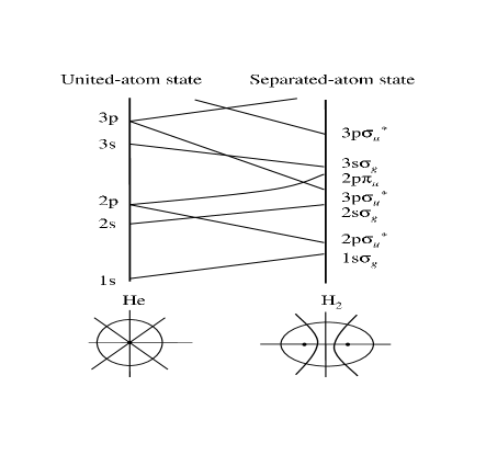
Figure 18: Schematic correlation diagram for He, the united atom limit, and H₂, the separated-atom case.

Recall the correlation diagram for H₂ molecule shown in Fig. 18 ScullyEtAl . A typical form of the trial wave function for H₂, e.g., may be represented as

$$\psi=[c_{1}\widetilde{\psi}_{H_{2},1s\sigma}+c_{2}\widetilde{\psi}_{H_{2},2p\sigma}]f(r_{12}),$$ (VI.52)

where $\widetilde{\psi}_{H_{2},1s\sigma}$ and $\widetilde{\psi}_{H_{2},2p\sigma}$ are chosen to be, respectively,

$$\left.\begin{array}[]{l}\widetilde{\psi}_{H_{2},1s\sigma}=\psi_{H^{+}_{2},1\sigma}(1)\psi_{H^{+}_{2},1\sigma}(2),\\ \widetilde{\psi}_{H_{2},2p\sigma}=\psi_{H^{+}_{2},2p}(1)\psi_{H^{+}_{2},2p}(2).\end{array}\right\}$$ (VI.53)

¿From (VI.52) and (VI.53), we see that the trial wave function (VI.52)

• is uncorrelated if $f(r_{12})\equiv 1$. If $f(r_{12})$ has explicit dependence on $r_{12}$, then (VI.52) is correlated. A simple choice of $f(r_{12})$ was

  $$f(r_{12})=1+\frac{1}{2}r_{12},$$ (VI.54)

  in Scully, et al. ScullyEtAl , but many such correlation functions $f$ satisfying the interelectronic cusp condition as given in Subsection V.B may be used also;

• has configuration interaction if $c_{1}c_{2}\neq 0$ in (VI.52).

It is found by ScullyEtAl that

• for uncorrelated orbitals and without configuration interaction, i.e., $f(r_{12})\equiv 1$ and $c_{2}=0$ in (VI.52), the choice of

  $$\psi_{H^{+}_{2},1\sigma}(j)={\mathcal{N}}e^{-\alpha_{1}\lambda_{j}}[1+B_{2}P_{2}(\mu_{j})],\qquad j=1,2,$$ (VI.55)

  in (VI.53)₁, where $P_{2}$ is a Legendre polynomial, gives the binding energy $E_{B}=0.132$ a.u.$=3.59$ eV for H₂. Here, ${\mathcal{N}}$ is a normalization constant, and $\alpha_{1}$ and $B_{2}$ are two variational parameters.

• for correlated orbitals but without configuration interaction, i.e., $f(r_{12})=1+\frac{1}{2}r_{12}$ and $c_{2}=0$ in (VI.52), the choice of (VI.55) yields the binding energy $E_{B}=0.1710$ a.u.$=4.653$ eV for H₂. The choice $f(r_{12})=1+\kappa r_{12}$, where $\kappa$ is a variational parameter, slightly improves the answer and gives $E_{B}=0.1713$ a.u.$=4.661$ eV.

• for correlated orbitals with configuration interaction, i.e., $f(r_{12})=1+\frac{1}{2}r_{12}$ and $c_{1}c_{2}\neq 0$ in (VI.52), the choice of (VI.55) along with

  $$\psi_{H^{+}_{2},2p}(j)={\mathcal{N}}e^{-\alpha_{2}\lambda_{j}}[P_{1}(\mu_{j})+B_{3}P_{3}(\mu_{j})]$$ (VI.56)

  in (VI.53) ($\alpha_{1}$, $B_{2}$, $\alpha_{2}$ and $B_{3}$ are variational parameters) yields the binding energy $E_{B}=0.1712$ a.u.$=4.658$ eV. For the correlation factor $f(r_{12})$ with the variational parameter $\kappa$ we obtain $E_{B}=0.1721$ a.u.$=4.682$ eV.

What is quite striking here is that if, instead of (VI.55), we choose a finer two-centered orbital

$$\psi_{H^{+}_{2},1\sigma}(j)={\mathcal{N}}e^{-\alpha_{1}\lambda_{j}}[1+B_{2}P_{2}(\mu_{j})+B_{4}P_{4}(\mu_{j})],\qquad j=1,2,$$ (VI.57)

and perform calculations using three variational parameters $\alpha_{1}$, $B_{2}$ and $B_{4}$, then numerical results manifest that $B_{2}$ totally dominates $B_{4}$, with a ratio $|B_{4}/B_{2}|\approx 2\times 10^{-3}$. This shows that the simple orbital (VI.52) with (VI.55) is able to capture the essence of chemical bonding of H₂ with very good accuracy.

For a heteronuclear molecule such as HeH⁺, a simple adaptation of the above scheme works equally well. Nevertheless, the authors have found that for large $R$, more terms involving both $\lambda$ and $\mu$ variables should be included in (VI.55), such as

$$\psi_{H^{+}_{2},1\sigma}(j)={\mathcal{N}}e^{-\alpha_{1}\lambda_{j}}[1+B_{2}P_{2}(\mu_{j})+\cdots+B_{2m}P_{m}(\mu_{j})][1+A_{1}L_{1}(x_{j})+\cdots+A_{n}L_{n}(x_{j})],\quad(x_{j}=2\alpha_{1}(\lambda_{j}-1)),$$ (VI.58)

where $L_{n}(x)$ are Laguerre polynomials, so that good accuracy can be maintained in the calculation of $E$.

Another choice of simple two-centered wave functions, in the same spirit of this subsection, was given by Patil P , where he has generalized the one-centered Guillemin–Zener type one-centered molecular orbitals (see Item (3)) by considering the gerade state

$$\psi_{g}=N(1+b\lambda)^{\beta}e^{-a\lambda}\cosh(a\mu)$$ (VI.59)

and ungerade state

$$\psi_{u}=N(1+b\lambda)^{\beta}e^{-a\lambda}\sinh(a\mu)$$ (VI.60)

for H${}^{+}_{2}$ (or any homonuclear) ionic orbitals. Asymptotic behavior of H${}^{+}_{2}$-like orbitals can be built in through $\beta$, which plays the same role as $\beta$ in the Jaffé solution (IV.22).

(1)  Le Sech’s simplification of integrals involving cross-terms of correlated wave functions

Siebbeles and Le Sech SL developed an ingenious approach to the evaluation of energy by applying integration by parts (or, Green’s Theorem) to avoid the quadratures of cross terms of the type

$$\nabla_{i}(\Phi_{i}\Phi_{j})\cdot\nabla_{i}f,\qquad i,j=1,2,$$ (VI.61)

where $f$ is a correlation function, and $\Phi_{i}\Phi_{j}$ is a product of two-centered orbitals. This is a fine feature of their approach.

They choose wave functions of the form

$$\psi(\boldsymbol{r}_{1},\boldsymbol{r}_{2})=\phi(1,2)\Omega(1,2),$$ (VI.62)

where $\Omega(1,2)$ plays the role of the correlation function (but may be more general than the) $f$ discussed in (VI.52), while

$$\phi(1,2)=\Phi(1)\Phi(2)$$ (VI.63)

where $\Phi(i)$, $i=1,2$, are the Hylleraas-type two-centered orbitals; cf. (VI.77) below. Note here that each of $\Phi_{1}$ and $\Phi_{2}$ can have higher order molecular configurations such as $2s\sigma_{g}$, $3p\sigma_{u}$, $3d\sigma_{g}$ and $4f\sigma_{u}$ (in the computation of He, e.g., in Le ).

Let the diatomic molecule’s Hamiltonian be

$$H=-\frac{1}{2}(\nabla^{2}_{1}+\nabla^{2}_{2})+V(1,2),$$ (VI.64)

where

$$V(1,2)=\widetilde{V}(1,2)+\frac{1}{r_{12}}$$ (VI.65)

with

$$\widetilde{V}(1,2)=-\left(\frac{Z_{a}}{r_{1a}}+\frac{Z_{b}}{r_{1b}}+\frac{Z_{a}}{r_{2a}}+\frac{Z_{b}}{r_{2b}}\right).$$ (VI.66)

Let $\Phi_{n}(i)$, $i=1,2$, be eigenstates of the two center problem

$$\left(-\frac{1}{2}\nabla^{2}_{i}-\frac{Z_{a}}{r_{ia}}-\frac{Z_{b}}{r_{ib}}\right)\Phi_{n}(i)=\epsilon_{n}\Phi_{n}(i),\qquad i=1,2.$$ (VI.67)

Denote $\phi_{j}(1,2)$ to be solutions of

$$\left[-\frac{1}{2}\left(\nabla^{2}_{1}+\nabla^{2}_{2}\right)+\widetilde{V}(1,2)\right]\phi_{j}(1,2)=E_{j}\phi_{j}(1,2).$$ (VI.68)

Then

$$\phi_{j}(1,2)\equiv\Phi_{n_{1}}(1)\Phi_{n_{2}}(2)\cdot\frac{1}{\sqrt{2}}[\alpha(1)\beta(2)-\alpha(2)\beta(1)]$$ (VI.69)

satisfies (VI.68) with

$$E_{j}=\epsilon_{n_{1}}+\epsilon_{n_{2}}.$$ (VI.70)

Now consider a trial wave function for (VI.64) in the form

$$\phi(1,2)\Omega(1,2)$$

where $\phi(1,2)$ is of the form (VI.69) while $\Omega(1,2)$ is intended to model the Coulombic repulsive effect from the $1/r_{12}$ term and, therefore, plays a similar role as (but may be more general than) the correlation function $f(r_{12})$. Without loss of generality, $\phi(1,2)$ and $\Omega(1,2)$ are assumed to be real.

Denote the 6-dimensional Laplacian

$$\nabla^{2}_{6}\equiv\nabla^{2}_{1}+\nabla^{2}_{2}.$$

Consider the matrix element

$$H_{ij} \equiv\langle\phi_{i}\Omega|-\frac{1}{2}\nabla^{2}_{6}+V(1,2)|\phi_{j}\Omega\rangle=\int\limits_{{\mathbb{R}}^{3}}\int\limits_{{\mathbb{R}}^{3}}d\boldsymbol{r}_{1}d\boldsymbol{r}_{2}\left[-\frac{1}{2}\phi_{i}\Omega\nabla^{2}_{6}(\phi_{j}\Omega)+\phi_{i}\phi_{j}\Omega^{2}V(1,2)\right]$$

$$=\iint d\boldsymbol{r}_{1}d\boldsymbol{r}_{2}\left[-\frac{1}{2}(\Omega^{2}\phi_{i}\nabla^{2}_{6}\phi_{j}+\phi_{i}\phi_{j}\Omega\nabla^{2}_{6}\Omega+\underbrace{2\phi_{i}\Omega\nabla_{6}\phi_{j}\cdot\nabla_{6}\Omega}_{{\mathcal{T}}_{1}})+\phi_{i}\phi_{j}\Omega^{2}V(1,2)\right].$$ (VI.71)

To treat ${\mathcal{T}}_{1}$, write

$${\mathcal{T}}_{1}=2\phi_{i}\Omega\nabla_{6}\phi_{j}\cdot\nabla_{6}\Omega=\phi_{i}\nabla_{6}\phi_{j}\cdot\nabla_{6}(\Omega^{2}),$$

and note through an easy verification the following:

$$2\phi_{i}\nabla\phi_{j}\cdot\nabla(\Omega^{2}) =-[\phi_{i}\phi_{j}\nabla^{2}(\Omega^{2})+\Omega^{2}\nabla\cdot(\phi_{i}\nabla\phi_{j}-\phi_{j}\nabla\phi_{i})]$$

$$\quad+\nabla\cdot[\phi_{i}\phi_{j}\nabla(\Omega^{2})+(\phi_{i}\nabla\phi_{j}-\phi_{j}\nabla\phi_{i})\Omega^{2}].$$ (VI.72)

But the LHS of (VI.72) is equal to twice of ${\mathcal{T}}_{1}$. So we now substitute one-half of the RHS of (VI.72) for ${\mathcal{T}}_{1}$ in (VI.71), obtaining

$$H_{ij} =\iint d\boldsymbol{r}_{1}d\boldsymbol{r}_{2}\Big{[}\underbrace{-\frac{1}{2}(\Omega^{2}\phi_{i}\nabla^{2}_{6}\phi_{j}}_{{\mathcal{T}}_{2}}+\phi_{i}\phi_{j}\Omega\nabla^{2}_{6}\Omega)$$

$$\quad+\underbrace{\frac{1}{4}(\phi_{i}\phi_{j}\nabla^{2}_{6}(\Omega^{2})+\Omega^{2}\nabla_{6}\cdot(\phi_{i}\nabla_{6}\phi_{j}}_{{\mathcal{T}}_{3}}-\phi_{j}\nabla_{6}\phi_{i}))+\phi_{i}\phi_{j}\Omega^{2}V(1,2)\Big{]},$$ (VI.73)

where the divergence term $\nabla\cdot[\cdots]$ in (VI.72) disappears after integration in the 6-dimensional space provided that $\phi_{i},\phi_{j},\nabla(\Omega^{2})$ and $\Omega^{2}$ decay fast enough as $|\boldsymbol{r}_{1}|$, $|\boldsymbol{r}_{2}|\to\infty$. The RHS of (VI.73) is further simplified by utilizing

$$\frac{1}{4}\nabla^{2}(\Omega^{2})=\frac{1}{2}|\nabla\Omega|^{2}+\frac{1}{2}\Omega(\nabla^{2}\Omega),$$

and by combining ${\mathcal{T}}_{2}$ with ${\mathcal{T}}_{3}$ terms therein, leading to

$$H_{ij}=\iint d\boldsymbol{r}_{1}d\boldsymbol{r}_{2}\left\{\frac{1}{2}\phi_{i}\phi_{j}|\nabla_{6}\Omega|^{2}-\frac{1}{4}\Omega^{2}[\phi_{i}\nabla^{2}_{6}\phi_{j}+\phi_{j}\nabla^{2}_{6}\phi_{i}]+\phi_{i}\phi_{j}\Omega^{2}V(1,2)\right\}.$$ (VI.74)

Now, with $\phi$ satisfying (VI.68) we obtain

$$H_{ij}=\iint d\boldsymbol{r}_{1}d\boldsymbol{r}_{2}\left\{\phi_{i}\phi_{j}\Omega^{2}\left[\frac{1}{2}(E_{i}+E_{j})+\frac{1}{r_{12}}\right]+\frac{1}{2}\phi_{i}\phi_{j}|\nabla_{6}\Omega|^{2}\right\}.$$ (VI.75)

Comparing (VI.75) with (VI.71), we see that all the cross-derivative terms $\nabla_{6}\phi_{j}\cdot\nabla_{6}\Omega$ have been eliminated, and the only “burden of differentiation” has been placed only on $|\nabla_{6}\Omega|^{2}$ in (VI.75).

If we choose $\Omega=1+\frac{1}{2}r_{12}$, then $|\nabla_{6}\Omega|^{2}=|\nabla_{1}\Omega|^{2}+|\nabla_{2}\Omega|^{2}=1/2$ and (VI.75) becomes

$$H_{ij}=\iint d\boldsymbol{r}_{1}d\boldsymbol{r}_{2}\left\{\phi_{i}\phi_{j}\Omega^{2}\left[\frac{1}{2}(E_{i}+E_{j})+\frac{1}{r_{12}}\right]+\frac{1}{4}\phi_{i}\phi_{j}\right\}.$$ (VI.76)

But $\Omega$ doesn’t have to be chosen as $\Omega=1+\frac{1}{2}r_{12}$. Le Sech has preferred a special form of $\Omega$ as given in (VB.(2)). Note that $\epsilon_{g}$ and $\epsilon_{u}$ can be used as variational parameters, so can be $d$ in (VB.(2)). In a personal communication from Le Sech to Scully (9/6/2004), Le Sech pointed out that the trial wave functions in the form of (VI.62) with $\Omega(1,2)$ chosen as (VB.(2)) is particularly suitable for the diffusion Monte Carlo method lesechetal1 .

Regarding the two-centered orbitals $\Phi_{n_{1}}(1)$ and $\Phi_{n_{2}}(2)$ in (VI.67) and (VI.69), Aubert–Frécon and Le Sech (A-FL, , (4)) used a truncated summation from the Hylleraas series solution, cf. (IV.30):

$$\Phi=\Phi(\lambda,\mu,\phi)=\sum^{K}_{k=m}f^{m}_{k}Y^{m}_{k}(\mu,\phi)\sum^{N}_{n=0}c_{n}e^{-p(\lambda-1)}[2p(\lambda-1)]^{m/2}L^{m}_{n}(2p(\lambda-1)),$$ (VI.77)

where $p$ is used as a variational parameter, and $f^{m}_{k}$ and $c_{n}$ are coefficients which can be determined from the Killingbeck procedures Ki .

(2)  Generalized correlated or uncorrelated two-centered wave functions

The two-centered orbitals we have been using in this section to build up the molecular orbitals, whether they be correlated, uncorrelated, with or without configuration interaction, have been heavily influenced by the classic solutions due to Hylleraas and Jaffé, cf. (IV.30) and (IV.26). These two famous solutions were derived during the 1920s and 1930s with great ingenuity, their greatest advantages being that a 3-term recurrent relation of the series coefficients. The 3-term recurrences further lead to continued fractions which have enabled mathematicians to perform asymptotic analysis. That was during a time when no electronic computers were available and it was perhaps the only way to perform any theoretical analysis at all. Nowadays, fast computers are readily available so we don’t have to rely overly on 3-term recurrence relations. Five-term recurrence relations are just as good and can be treated with relative ease also by the Killingbeck algorithm Ki , for example.

Recall that for the single-electron, two-centered heteronuclear problem, separation of variables leads to

$$[(\lambda^{2}-1)\Lambda^{\prime}]^{\prime}+\left[A+2R_{1}\lambda-p^{2}\lambda^{2}-\frac{m^{2}}{\lambda^{2}-1}\right]\Lambda=0, (R_{1}\equiv R(Z_{a}+Z_{b})/2)$$ (VI.78)

$$[(1-\mu^{2})M^{\prime}]^{\prime}+\left[-A-2R_{2}\mu+p^{2}\mu^{2}-\frac{m^{2}}{1-\mu^{2}}\right]M=0, (R_{2}\equiv R(Z_{a}-Z_{b})/2).$$ (VI.79)

The appearances of the above two equations suggest the ansatz

$$\Lambda(\lambda)=\sum^{\infty}_{k=0}f_{k,1}P^{m}_{k}(\lambda),\quad M(\mu)=\sum^{\infty}_{k=0}f_{k,2}P^{m}_{k}(\mu),$$ (VI.80)

where $P_{k}^{m}(\lambda)$ are the associated Legendre polynomials. Substituting (VI.80) into (VI.78) and (VI.79) and equate coefficients of $P^{m}_{k}(\lambda)$ and $P^{m}_{k}(\mu)$ to zero, see Appendix L, we obtain 5-term recurrence relations

$$A_{kj}f_{k-2,j}+B_{kj}f_{k-1,j}+C_{kj}f_{k,j}+D_{kj}f_{k+1,j}+E_{kj}f_{k+2,j}=0,\qquad k=1,2;j=0,1,2,\ldots,$$ (VI.81)

where

$$\left.\begin{array}[]{l}A_{k1}=A_{k2}=\dfrac{p^{2}(k-m-1)(k-m)}{(2k-3)(2k-1)},\\ \vskip 6.0pt plus 2.0pt minus 2.0pt\cr B_{kj}=-\dfrac{2R_{j}(k-m)}{2k-1},\qquad j=1,2,\\ \vskip 6.0pt plus 2.0pt minus 2.0pt\cr C_{k1}=C_{k2}=-k(k+1)-A+\dfrac{p^{2}(k-m+1)(k+m+1)}{(2k+1)(2k+3)}+\dfrac{p^{2}(k-m)(k+m)}{(2k+1)(2k-1)}\\ \vskip 6.0pt plus 2.0pt minus 2.0pt\cr D_{kj}=-\dfrac{2R_{j}(k+m+1)}{2k+3},\qquad j=1,2,\\ \vskip 6.0pt plus 2.0pt minus 2.0pt\cr E_{k1}=E_{k2}=\dfrac{p^{2}(k+m+1)(k+m+2)}{(2k+3)(2k+5)}.\end{array}\right\}$$ (VI.82)

The two-centered orbitals derived above differ from those of Hylleraas and Jaffé. The ansatz (VI.80) is not the only way to obtain two-centered orbitals. It is possible to derive several other solutions in different forms using different orthogonal polynomials. Numerical results indicate that these two-centered orbitals here give accuracy compatible to that corresponding to Hylleraas and Jaffé type solutions.

(3)  Numerical algorithm

In contrast to the explicit analytic formulas for the quadratures of James–Coolidge wave functions given in VI.D and in the affiliated Appendices J and K, here the integrals will be computed using the Gaussian quadrature routines. (The analytic formulas given earlier in VI.D can then be compared with those obtained here as a good check.) For the two-electron problem, the number of coordinates are six, so that the energy calculation requires the 6-dimensional integration. Using the cylindrical symmetry, we can reduce two angular variables to one.

The next simplification is the choice of the wave functions. If we only restrict the wave functions to be the James–Coolidge type, the 5-dimensional integration can be divided as one two-dimensional integration and two three-dimensional integration. However, if we include the exponential function of inter-electron distance, that is $e^{-\kappa r_{12}}$, this 5-dimensional integration should be evaluated as multidimensional integration, and the numerical accuracy should be carefully investigated.

Here, we only restrict the wave functions to be the James–Coolidge type. The usual integration has the following form.

$$\int\cdots\int\Lambda_{1}(\lambda_{1})\Lambda_{2}(\lambda_{2})M_{1}(\mu_{1})M_{2}(\mu_{2})\Phi(\phi_{1}-\phi_{2})r_{12}^{n}d\lambda_{1}d\lambda_{2}d\mu_{1}d\mu_{2}d\phi_{1}d\phi_{2}$$ (VI.83)

Using the $r_{12}^{2}$-identity, cf. (VI.31), the exponent of $r_{12}$ can be reduced into 0 or -1. For $n=0$, the whole integration is divided into only 5 one-dimensional integrations. However, for $1/r_{12}$, by the Neumann expansion the form of wave function includes sum of Legendre Polynomials with proper coefficients; cf. (VI.39). Especially, the form of the $\lambda$-part is

$$P(\lambda_{<})Q(\lambda_{>})=\left\{\begin{array}[]{lll}P(\lambda_{1})Q(\lambda_{2}),&&\lambda_{1}<\lambda_{2},\\ P(\lambda_{2})Q(\lambda_{1}),&&\lambda_{2}>\lambda_{1}.\end{array}\right.$$ (VI.84)

This makes the form of integration over the $\lambda$ variable as

$$\int^{\infty}_{0}\int^{\infty}_{0}\cdots=\int^{\infty}_{0}\int^{\lambda_{1}}_{0}\cdots+\int^{\infty}_{0}\int^{\infty}_{\lambda_{1}}\cdots$$ (VI.85)

The implementation of these numerical integration is automated by standard computer software. Let us describe the numerics for a homonuclear dimer H₂ molecule and a heteronuclear dimer HeH⁺ molecular ion.

The approximation of wave function of two-electron system into a multiplication of one-electron system can be easily made in the natural orbit expansion

$$\Psi(\mathbf{r}_{1},\mathbf{r}_{2})=\sum c_{k}\chi_{k}(\mathbf{r}_{1})\chi_{k}(\mathbf{r}_{2})$$ (VI.86)

where $\chi_{k}(\mathbf{r}_{1})$ is the wave function of one-electron two-center problem.

For the ground state, it’s well-known that $c_{1}\sim 1$, or

$$\Psi(\mathbf{r}_{1},\mathbf{r}_{2})\simeq\chi_{1}(\mathbf{r}_{1})\chi_{1}(\mathbf{r}_{2}).$$ (VI.87)

There are a few alternatives to approximate the $\chi_{1}(\mathbf{r}_{1})$. One is using the exact solution of one-electron two-center problem, $1s\sigma_{g}$ state. The Jaffe’s form is

$$\chi_{1}(\mathbf{r}_{1})=e^{-\alpha\lambda}(1+\lambda)^{\sigma}\sum_{n}g_{n}\left(\frac{\lambda-1}{\lambda+1}\right)^{n}\sum_{m}f_{2m}P_{2m}(\mu),$$ (VI.88)

cf. (IV.26).

And the other is Patil’s wave function

$$\chi_{1}(\mathbf{r}_{1})=(1+b\lambda)^{\beta}e^{-\alpha_{P}\lambda}\cosh(a\mu);\quad\text{cf.\ \eqref{eq6.27a}.}$$ (VI.89)

We may also include configuration interaction, such as

$$\Psi(\mathbf{r}_{1},\mathbf{r}_{2})=c_{1}\chi_{1}(\mathbf{r}_{1})\chi_{1}(\mathbf{r}_{2})+c_{2}\chi_{2}(\mathbf{r}_{1})\chi_{2}(\mathbf{r}_{2})$$ (VI.90)

where $\chi_{1}$ is $1s\sigma_{g}$ state and $\chi_{2}$ is $2p\sigma_{u}$ state.

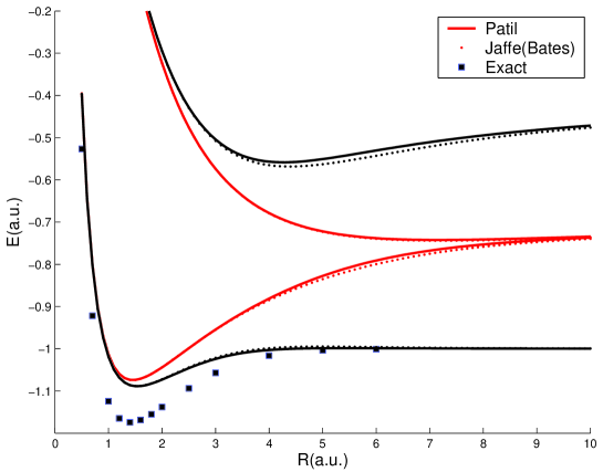
Figure 19: Comparison of potential curves of the H₂ molecule computed with no correlation factor using the exact solution of the one-electron wave function (VI.88) (small dots) and the Patil’s wave function (VI.89) (solid line). The inner (outer) curves are the result without (with) configuration interaction. Squares are the “exact” ground state $E(R)$ from Ref. Kolo60 . Upper curves correspond to “excited states”.

The result is shown in Fig. 19. Before the diagonalization (that is, CI), the asymptotic behavior of the ground state $E(R)$ is monotonically increasing. By diagonalizing, the behavior at large $R$ becomes almost flat, however, $E(R)$ is slightly above the exact asymptotic value, -1 (htr).

Next, we perform computations with correlation by using $f(r_{12})=1+\frac{1}{2}r_{12}$. Improvement can be readily seen in Fig. 20 which is much closer to the exact calculation done by Kolos Kolo60 .

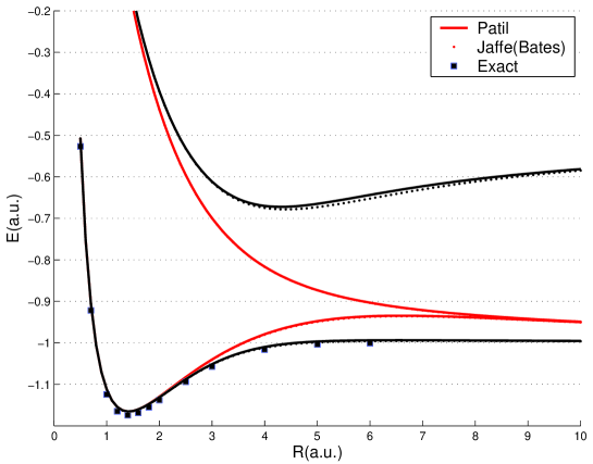
Figure 20: Same computations as with Fig. 19, but with the correlation factor.

In the calculations below (Figs. 19 and 20), “exact” solutions of H${}^{+}_{2}$-solutions were used (whose coefficients are obtained through truncated Killingbeck Ki procedures). Instead, one can use (VI.55), (VI.56), (VI.57) by optimizing the coefficients $\alpha$ and $B$ therein, or, for the Patil’s wave function, by optimizing the coefficients $a$ and $\beta$ in (VI.59) and (VI.60). By doing so, we obtain the energy curve of the ground state as shown in Figs. 21 and 22, respectively. The energy curves are improved over a wide range of $R$ values, and we obtain the binding energy of $0.171$ a.u.$=4.65$ eV, close to the experimental value. However, $E(R)$ in Fig. 21 overshoots the dissociation limit.

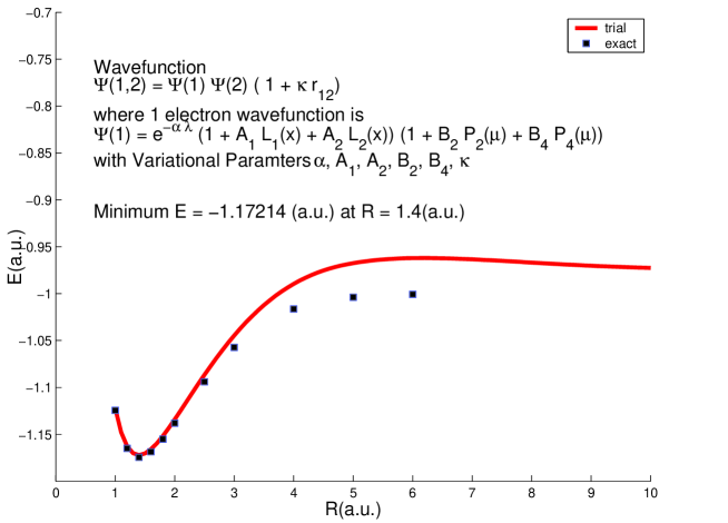
Figure 21: Ground state potential energy curve of the H₂ obtained using the truncated exact wave functions of one-electron system with the correlation factor and several variational parameters. The curve yields the binding energy of $E_{B}=-0.1721$ a.u.$=4.684$ eV. Squares are the “exact” ground state $E(R)$.

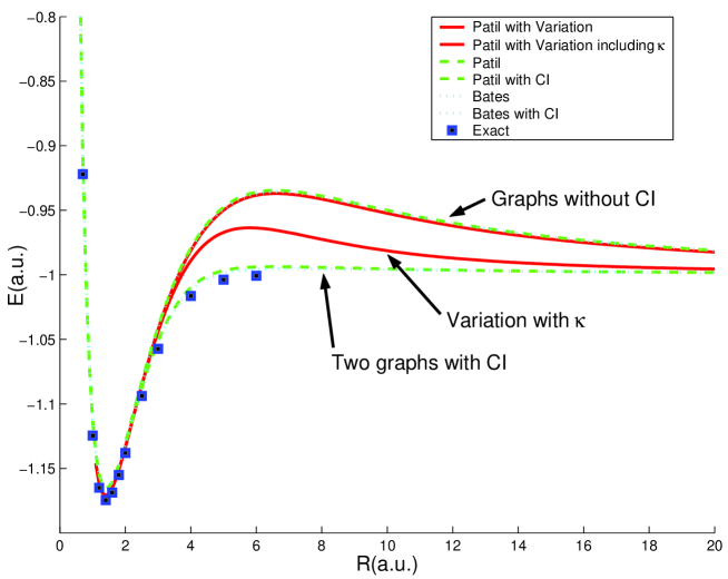
Figure 22: Ground state potential curve of H₂ computed from the Patil’s wave function with the correlation factor and variational parameters. The curve yields the binding energy of $E_{B}=-0.1713$ a.u.$=4.662$ eV. Squares are the “exact” ground state $E(R)$.

VII Alternative approaches

VII.1 Improvement of Hartree–Fock results using the Bohr model

The Bohr model can also be applied to calculate the correlation energy for molecules and then improve the HF treatment. Fig. 23 shows the ground state potential curve for H₂ molecule calculated in the Bohr-HF approximation. Such an approximation omits the electron repulsion term $1/r_{12}$ in finding the electron configuration from Eq. (I.2). The difference between the Bohr and Bohr-HF potential curves yields the correlation energy plotted in the insert of Fig. 23.

Figure 23: Ground state $E(R)$ for the H₂ molecule in the Bohr and Bohr-HF models. Insert shows the correlation energy as a function of $R$.

In Fig. 24 we draw the ground state $E(R)$ for the H₂ molecule obtained with the Heitler–London trial function that has the form of the combination of the atomic orbitals Slat63 :

$$\Psi=C\left\{\exp[-\alpha(r_{a1}+r_{b2})]+\exp[-\alpha(r_{b1}+r_{a2})]\right\},$$

where $\alpha$ is a variational parameter. Addition of the correlation energy from Fig. 23 improves the Heitler–London result and shifts $E(R)$ close to the “exact” values. The improved potential curve yields the binding energy of 4.63 eV.

Figure 24: Ground state energy $E(R)$ of the H₂ molecule in the Heitler–London method and the improved $E(R)$ after the addition of the correlation energy. Dots are the “exact” result from Kolo60 .

VII.2 Dimensional scaling

Dimensional scaling offers promising new computational strategies for the study of few electron systems. This is exemplified by recent applications to atoms, as well as H${}_{2}^{+}$ and H₂ molecules Hers92 ; Svid04 . D-scaling emulates a standard method of quantum chromodynamics Witt80 , by generalizing the Schrödinger equation to D dimensions and rescaling coordinates Hers92 . The $D\rightarrow\infty$ limit corresponds to infinitely heavy electrons and reduces to a classic electrostatic problem of finding an electron configuration that minimizes a known effective potential.

We start from the Schrödinger equation $\hat{H}\Psi=E\Psi$ for a two particle wave function $\Psi({\bf r}_{1},{\bf r}_{2})$. The H₂ Hamiltonian in atomic units reads

$$\hat{H}=-\frac{1}{2}\nabla_{1}^{2}-\frac{1}{2}\nabla_{2}^{2}+V(\rho_{1},\rho_{2},z_{1},z_{2},\phi,R),$$

where the Coulomb potential energy $V$ is given by Eq. (I.1). In a traditional dimensional scaling approach the Laplacian is treated in D-dimension and the wave function is transformed by incorporating the square root of the Jacobian via $\Psi\rightarrow J^{-1/2}\Phi$, where $J=(\rho_{1}\rho_{2})^{D-2}(\sin\phi)^{D-3}$ in cylindrical coordinates, and $\phi$ is the dihedral angle specifying relative azimuthal orientation of electrons about the molecular axis Fran88 . D-scaling in spherical coordinates is discussed in Appendix M. On scaling the coordinates by $f^{2}$ and the energy by $1/f^{2}$, with $f=(D-1)/2$, the Schrödinger equation in the limit $D\rightarrow\infty$ leads to minimization of the effective potential Fran88

$$E=\frac{1}{2}\left(\frac{1}{\rho_{1}^{2}}+\frac{1}{\rho_{2}^{2}}\right)\frac{1}{\sin^{2}\phi}+V(\rho_{1},\rho_{2},z_{1},z_{2},\phi,R).$$ (VII.1)

The obtained electron configuration is sometimes called the Lewis structure because it provides a rigorous version of the familiar electron-dot formulas introduced by Lewis in 1916 Lewi16 . Fig. 25 (upper curve) displays the $D\rightarrow\infty$ potential curve $E(R)$ that exhibits no binding and substantially deviates from the $D=3$ “exact” energy (dots). In the limit $D\rightarrow 1$ the dimensional scaling reduces the Hamiltonian to the delta function model Dore87

$$\hat{H}=-\frac{1}{2}\left(\frac{d^{2}}{dx_{1}^{2}}+\frac{d^{2}}{dx_{2}^{2}}\right)-\delta\left(x_{1}+\frac{R}{2}\right)-\delta\left(x_{1}-\frac{R}{2}\right)-\delta\left(x_{2}+\frac{R}{2}\right)-\delta\left(x_{2}-\frac{R}{2}\right)+\delta\left(x_{1}-x_{2}\right).$$ (VII.2)

A variational solution of the one dimensional wave equation Lapi75 is pictured in Fig. 25 (lower curve). Also shown is an approximation to $E(R)$ for $D=3$ obtained by interpolating linearly in $1/D$ between the dimensional limits:

$$E_{3}(R)=\frac{2}{3}E_{\infty}(R)+\frac{1}{3}E_{1}(R).$$ (VII.3)

The interpolated $D=3$ curve exhibits binding which indicates the feasibility of extending dimensional interpolation to molecules.

Figure 25: Ground state energy $E(R)$ of the H₂ molecule in $D=\infty$, $D=1$ and three dimensional interpolation (solid lines). Dots show the “exact” D=3 energy from Kolo60 .

A proper choice of scaling can improve the method. Here we discuss a dimensional scaling transformation of the Schrödinger equation that yields the Bohr model of H₂ in the limit of infinite dimensionality Svid04 . For such a transformation, the large-D limit provides a link between the old (Bohr-Sommerfeld) and the new (Heisenberg-Schrödinger) quantum mechanics. The first-order correction in 1/D substantially improves the agreement with the exact ground state $E(R)$.

In the modified scaling the Laplacian depends on a continuous parameter $D$ as follows

$$\nabla^{2}=\frac{1}{\rho^{D-2}}\frac{\partial}{\partial\rho}\left(\rho^{D-2}\frac{\partial}{\partial\rho}\right)+\frac{1}{\rho^{2}}\frac{\partial^{2}}{\partial\phi^{2}}+\frac{\partial^{2}}{\partial z^{2}}.$$ (VII.4)

For $D=3$, Eq. (VII.4) reproduces the 3D Laplacian. On scaling the coordinates by $f^{2}$, the energy by $1/f^{2}$ (recalling $f=(D-1)/2$) and transforming the electronic wave function $\Psi$ by

$$\Psi=(\rho_{1}\rho_{2})^{-(D-2)/2}\Phi,$$ (VII.5)

the Schrödinger equation is recast as

$$(K+U+V)\Phi=E\Phi,$$ (VII.6)

where

$$K=-\frac{2}{(D-1)^{2}}\left\{\frac{\partial^{2}}{\partial\rho_{1}^{2}}+\frac{\partial^{2}}{\partial\rho_{2}^{2}}+\frac{\partial^{2}}{\partial z_{1}^{2}}+\frac{\partial^{2}}{\partial z_{2}^{2}}+\left(\frac{1}{\rho_{1}^{2}}+\frac{1}{\rho_{2}^{2}}\right)\frac{\partial^{2}}{\partial\phi^{2}}\right\},$$

$$U=\frac{(D-2)(D-4)}{2(D-1)^{2}}\left(\frac{1}{\rho_{1}^{2}}+\frac{1}{\rho_{2}^{2}}\right).$$ (VII.7)

In the $D\rightarrow\infty$ limit the derivative terms in $K$ are quenched. The corresponding energy $E_{\infty}$ for any given internuclear distance $R$ is then obtained simply as the minimum of an effective potential

$$E=\frac{1}{2}\left(\frac{1}{\rho_{1}^{2}}+\frac{1}{\rho_{2}^{2}}\right)+V(\rho_{1},\rho_{2},z_{1},z_{2},\phi,R).$$ (VII.8)

This is identical in form to that for the Bohr model, Eq. (I.2), and we thus obtain for $E_{\infty}(R)$ the same solutions depicted in Fig. 2. This result for $E_{\infty}(R)$ differs in an interesting way from that obtained in a traditional study of the $D\rightarrow\infty$ limit for the H₂ molecule Fran88 . Here, in order to connect with the Bohr model, it is necessary to incorporate only the radial portion of the Jacobian in transforming the electronic wave function via Eq. (VII.5). The customary practice, which employs the full Jacobian, introduces a factor of $1/(\sin^{2}\phi)$ into the centrifugal potential, as seen from Eq. (VII.1). The modified procedure yields directly a good zeroth-order approximation.

The ground state $E(R)$ can be substantially improved by use of a perturbation expansion in powers of $1/D$, developed by expanding the effective potential of Eq. (VII.8) in powers of the displacement from the minimum Hers92 ; for He and H${}_{2}^{+}$ this has yielded highly accurate results Good92 . Terms quadratic in the displacement describe harmonic oscillations about the minimum and give a $1/D$ correction to the energy. Anharmonic cubic and quartic terms give a $1/D^{2}$ contribution. For the He ground state energy (the $R=0$ limit for H₂) a first-order approximation yields Svid04 ; ff

$$E(0)=\frac{4E_{\infty}}{(D-1)^{2}}\left(1-\frac{0.1532}{D}\right),$$ (VII.9)

where $E_{\infty}=-3.062$ a.u. is the Bohr model He result Bohr1 ; Vlec22 . For $D=3$ Eq. (VII.9) improves the ground state energy of He to $E(0)=-2.906$ a.u., which differs by $0.07\%$ only from the “exact” value of $-2.9037$ a.u. Drak02 .

To evaluate the $1/D$ correction for arbitrary $R$, it is convenient to introduce new coordinates

$$\tilde{z}_{1}=\frac{1}{\sqrt{2}}(z_{1}-z_{2}),\qquad\tilde{z}_{2}=\frac{1}{\sqrt{2}}(z_{1}+z_{2}).\qquad$$

The effective potential of Eq. (VII.8) then has a minimum at $\rho_{1}=\rho_{2}=\rho_{0},$ $\phi=\pi,$ $\tilde{z}_{2}=0$. Along the coordinates $\rho_{1}$, $\rho_{2}$, $\tilde{z}_{2}$ and $\phi$ the potential has a single well structure no matter what the internuclear spacing $R$ is. However, along the $\tilde{z}_{1}$ direction at $R=1.2$ the potential changes shape from a single to a double well; such symmetry breaking is a typical feature exhibited at large D Shi01 . To avoid the inaccuracy of approximation by a single quadratic form one can solve the Schrödinger equation numerically along the $\tilde{z}_{1}$ direction for the exact potential and add contributions from the harmonic motion associated with the other coordinates $\rho_{1}$, $\rho_{2}$, $\tilde{z}_{2}$ and $\phi$. The result is shown in Fig. 26 Svid04 . The $1/D$ correction improves $E(R)$ and predicts the equilibrium separation to be $R_{e}=1.62$ with binding energy $E_{B}=4.38$ eV.

Figure 26: Ground state energy $E$ of H₂ molecule as a function of internuclear distance $R$ calculated within the dimensional scaling approach (solid lines) and the “exact” energy (dots).

VIII Conclusions and outlook

Many major topics on diatomic molecules, and some other atoms and molecules in general, have been addressed in this article, giving it a very “locally diverse” or perhaps a somewhat disjoint look. But a simple, “global” picture may be viewed and understood in/from the following diagram:

This “unification” is by no means an easy task. Nevertheless, it was a goal we somehow envisioned to achieve when this research was started and we hope we have made at least some success.

At present, in the study of ultrafast laser applications to chemical physics and molecular chemistry problems, there is a pressing need to understand the quantum-dynamical behavior of molecules and the associated properties of excited states and their computations. Many challenges are lying ahead and awaiting elegant solutions.

Appendices

Appendix A Separation of variables for the H${}_{2}^{+}$-like Schrödinger equation.

Let us consider (IV.13). Here we show how to separate the variables through the use of the ellipsoidal (or, prolate spheroidal) coordinates (see Fig. 9)

$$x=\frac{R}{2}\sqrt{(\lambda^{2}-1)(1-\mu^{2})}\ \cos\phi,\quad y=\frac{R}{2}\sqrt{(\lambda^{2}-1)(1-\mu^{2})}\ \sin\phi,\quad z=\frac{R}{2}\lambda\mu.$$ (A.1)

Note that the coordinates $\lambda,\mu$ and $\phi$ are orthogonal, and we have the first fundamental form

$$ds^{2}=dx^{2}+dy^{2}+dz^{2}=h^{2}_{\lambda}\ d\lambda^{2}+h^{2}_{\mu}\ d\mu^{2}+h^{2}_{\phi}\ d\phi^{2}$$

where

$$h^{2}_{\lambda} =\left(\frac{\partial x}{\partial\lambda}\right)^{2}+\left(\frac{\partial y}{\partial\lambda}\right)^{2}+\left(\frac{\partial z}{\partial\lambda}\right)^{2}=\frac{R^{2}}{4}\frac{1-\mu^{2}}{\lambda^{2}-1},$$

$$h^{2}_{\mu} =\left(\frac{\partial x}{\partial\mu}\right)^{2}+\left(\frac{\partial y}{\partial\mu}\right)^{2}+\left(\frac{\partial z}{\partial\mu}\right)^{2}=\frac{R^{2}}{4}\frac{\lambda^{2}-1}{1-\mu^{2}},$$

$$h^{2}_{\phi} =\left(\frac{\partial x}{\partial\phi}\right)^{2}+\left(\frac{\partial y}{\partial\phi}\right)^{2}+\left(\frac{\partial z}{\partial\phi}\right)^{2}=\frac{R^{2}}{4}(\lambda^{2}-1)(1-\mu^{2}).$$

Thus

$$\nabla^{2}\Psi =\frac{1}{h_{\lambda}h_{\mu}h_{\phi}}\left[\frac{\partial}{\partial\lambda}\left(\frac{h_{\mu}h_{\phi}}{h_{\lambda}}\frac{\partial}{\partial\lambda}\Psi\right)+\frac{\partial}{\partial\mu}\left(\frac{h_{\lambda}h_{\phi}}{h_{\mu}}\frac{\partial}{\partial\mu}\Psi\right)+\frac{\partial}{\partial\phi}\left(\frac{h_{\lambda}h_{\mu}}{h_{\phi}}\frac{\partial}{\partial\phi}\Psi\right)\right]$$

$$=\frac{4}{R^{2}(\lambda^{2}-\mu^{2})}\left\{\frac{\partial}{\partial\lambda}\left[(\lambda^{2}-1)\frac{\partial}{\partial\lambda}\right]+\frac{\partial}{\partial\mu}\left[(1-\mu^{2})\frac{\partial}{\partial\mu}\right]+\frac{\lambda^{2}-\mu^{2}}{(\lambda^{2}-1)(1-\mu^{2})}\frac{\partial^{2}}{\partial\phi^{2}}\right\}\Psi.$$ (A.2)

Note that through the coordinate transformation (A.1), we have

$$\left\{\begin{array}[]{l}\lambda=\dfrac{r_{a}+r_{b}}{R},\\ \vskip 3.0pt plus 1.0pt minus 1.0pt\cr\mu=\dfrac{r_{a}-r_{b}}{R},\end{array}\right.\qquad\text{equivalently,}\qquad\begin{array}[]{l}r_{a}=\dfrac{R}{2}(\lambda+\mu),\\ \vskip 3.0pt plus 1.0pt minus 1.0pt\cr r_{b}=\dfrac{R}{2}(\lambda-\mu).\end{array}$$ (A.3)

Also, we have $\lambda\geq 1,-1\leq\mu\leq 1$.

Write

$$\Psi=\Lambda(\lambda)M(\mu)\Phi(\phi).$$ (A.4)

$\Phi(\phi)$ must be periodic with period $2\pi$. Therefore

$$\Phi(\phi)=e^{im\phi},\qquad m=0,\pm 1,\pm 2,\ldots~{}.$$ (A.5)

Substitute (A.2), (A.4) and (A.5) into (IV.13), and then divide by $e^{im\phi}$:

$$-\frac{1}{2}\frac{4}{R^{2}(\lambda^{2}-\mu^{2})}\left\{\frac{\partial}{\partial\lambda}\left[(\lambda^{2}-1)\frac{\partial}{\partial\lambda}\Lambda\right]M+\frac{\partial}{\partial\mu}\left[(1-\mu^{2})\frac{\partial}{\partial\mu}M\right]\Lambda-\frac{(\lambda^{2}-\mu^{2})m^{2}}{(\lambda^{2}-1)(1-\mu^{2})}M\Lambda\right\}$$

$$-\frac{2}{R}\frac{Z_{b}}{\lambda+\mu}M\Lambda-\frac{2}{R}\frac{Z_{a}}{\lambda-\mu}M\Lambda+\frac{Z_{a}Z_{b}}{R}M\Lambda=EM\Lambda.$$ (A.6)

Further multiplying every term by $-\frac{R^{2}}{2}(\lambda^{2}-\mu^{2})$, we obtain

$$\frac{\partial}{\partial\lambda}\left[(\lambda^{2}-1)\frac{\partial}{\partial\lambda}\Lambda\right]M+\frac{\partial}{\partial\mu}\left[(1-\mu^{2})\frac{\partial}{\partial\mu}M\right]\Lambda-\frac{\lambda^{2}-\mu^{2}}{(\lambda^{2}-1)(1-\mu^{2})}m^{2}M\Lambda$$

$$+\underbrace{\left[RZ_{b}(\lambda-\mu)+RZ_{a}(\lambda+\mu)-\left(\frac{RZ_{a}Z_{b}}{2}-\frac{R^{2}E}{2}\right)(\lambda^{2}-\mu^{2})\right]}_{\left(\frac{R^{2}E}{2}-\frac{RZ_{a}Z_{b}}{2}\right)(\lambda^{2}-\mu^{2})+R[(Z_{a}+Z_{b})\lambda+(Z_{a}-Z_{b})\mu]}M\Lambda=0.$$ (A.7)

Set

$$p^{2}=\frac{1}{2}(-R^{2}E+RZ_{a}Z_{b})>0.$$ (A.8)

We have $p^{2}>0$ here due to the fact that we are mainly interested in the electronic states that are bound states, i.e., not ionized.

Let the constant of separation of variables be $A$. Then from (A.7) and (A.8) we obtain (IV.16) and (IV.17) in Subsection IV.B.

Appendix B The asymptotic expansion of $\boldsymbol{\Lambda(\lambda)}$ for large $\boldsymbol{\lambda}$

Here, we provide a quick proof of Eq. (IV.22). From (IV.19), we have

$$\Lambda^{\prime\prime}(\lambda)-p^{2}\Lambda(\lambda)=-\left\{\frac{2\lambda}{\lambda^{2}-1}\Lambda^{\prime}(\lambda)+\left[\frac{A+2R_{1}\lambda}{\lambda^{2}-1}-p^{2}\left(\frac{\lambda^{2}}{\lambda^{2}-1}-1\right)-\frac{m^{2}}{(\lambda^{2}-1)^{2}}\right]\Lambda(\lambda)\right\}.$$ (B.1)

We now find the Laurent expansions of the coefficient functions on the right-hand side of (B.1) as follows:

$$\frac{2\lambda}{\lambda^{2}-1}=\frac{2}{\lambda}+\frac{0}{\lambda^{2}}+\frac{2}{\lambda^{3}}+\frac{0}{\lambda^{4}}+\frac{2}{\lambda^{5}}+\cdots,$$

$$\frac{A+2R_{1}\lambda}{\lambda^{2}-1} =\frac{1}{\lambda^{2}}(A+2R_{1}\lambda)\left(1+\frac{1}{\lambda^{2}}+\frac{1}{\lambda^{4}}+\cdots\right)$$

$$=\frac{2R_{1}}{\lambda}+\frac{A}{\lambda^{2}}+\frac{2R_{1}}{\lambda^{3}}+\frac{A}{\lambda^{4}}+\cdots,$$

$$-p^{2}\left(\frac{\lambda^{2}}{\lambda^{2}-1}-1\right) =\frac{0}{\lambda}-\frac{p^{2}}{\lambda^{2}}+\frac{0}{\lambda^{3}}-\frac{p^{2}}{\lambda^{4}}\pm\cdots$$

$$-\frac{m^{2}}{(\lambda^{2}-1)^{2}} =\frac{0}{\lambda}+\frac{0}{\lambda^{2}}+\frac{0}{\lambda^{3}}-\frac{m^{2}}{\lambda^{4}}+\frac{0}{\lambda^{5}}-\frac{2m^{2}}{\lambda^{6}}\pm\cdots~{}.$$

¿From these expansions above, we now use the ansatz

$$\Lambda(\lambda)=a_{0}e^{-p\lambda}\lambda^{\beta}\left(1+\frac{c_{1}}{\lambda}+\frac{c_{2}}{\lambda^{2}}+\cdots\right)$$

by substituting it into (B.1) and equating all the coefficients of $\lambda^{-n}$ to zero for $n=0,1,2,\ldots$ . We easily obtain

$$\beta=\frac{R_{1}}{p}-1,\quad c_{1}=\frac{p^{2}-\beta^{2}-2\beta}{2R_{1}-2p\beta-p}.$$

All the other coefficients $c_{n}$ can be determined in a straightforward way. Note that the asymptotic expansion (IV.22) also gives

$$\Lambda(\lambda)-a_{1}e^{-p\lambda}\lambda^{\beta}\sum^{n}_{j=0}\frac{c_{j}}{\lambda^{j}}=\mathcal{O}(e^{-p\lambda}\lambda^{\beta(n+1)}),\text{ for }\lambda\gg 1.$$ (B.2)

Appendix C The asymptotic expansion of $\boldsymbol{\Lambda(\lambda)}$ as $\boldsymbol{\lambda}\rightarrow 1$

Here we provide a proof of Eq. (IV.23). Multiply (IV.18) by $(\lambda-1)/(\lambda+1)$ and rewrite it as

$$0 =(\lambda-1)^{2}\Lambda^{\prime\prime}(\lambda)+\frac{2\lambda}{\lambda+1}(\lambda-1)\Lambda^{\prime}(\lambda)+\left[\frac{(A+2R_{1}\lambda-p^{2}\lambda^{2})}{\lambda+1}(\lambda-1)-\frac{m^{2}}{(\lambda+1)^{2}}\right]\Lambda(\lambda)$$

$$\approx(\lambda-1)^{2}\Lambda^{\prime\prime}(\lambda)+(\lambda-1)\Lambda^{\prime}(\lambda)-\frac{m^{2}}{4}\Lambda(\lambda),\text{ for }\lambda\approx 1.$$ (C.1)

A differential equation (such as (C.1)) set in the form

$$(x-1)^{2}y^{\prime\prime}(x)+(x-1)q(x)y^{\prime}(x)+r(x)y(x)=0,$$ (C.2)

near $x=1$, where $q(x)$ and $r(x)$ are analytic functions at $x=1$, is said to have a regular singular point at $x=1$. The solution’s behavior near $x=1$ hinges largely on the roots $\nu$ of the indicial equation

$$\nu(\nu-1)+q(1)\nu+r(1)=0$$ (C.3)

because the solution $y(x)$ of (C.2) is expressible as

$$y(x)=b_{1}(x-1)^{\nu_{1}}\sum^{\infty}_{k=0}c_{k}(x-1)^{k}+b_{2}(x-1)^{\nu_{2}}\sum^{\infty}_{k=0}d_{k}(x-1)^{k},\qquad(c_{0}=d_{0}=1),$$

where $\nu_{1}$ and $\nu_{2}$ are the two roots of the indicial equation (C.3), under the assumptions that

$$\nu_{1}>\nu_{2},\quad\nu_{1}-\nu_{2}\quad\text{is not a positive integer}.$$ (C.4)

However, if (C.4) is violated, then there are two possibilities and two different forms of solutions arise:

(a)  $\boldsymbol{\nu_{1}=\nu_{2}}$. Then

$$y(x) =b_{1}y_{1}(x)+b_{2}y_{2}(x),$$ (C.5)

where

$$y_{1}(x) =(x-1)^{\nu_{1}}\sum^{\infty}_{k=0}c_{k}(x-1)^{k},\quad(c_{0}=1)$$ (C.6)

and

$$y_{2}(x) =(x-1)^{\nu_{1}}\sum^{\infty}_{k=1}d_{k}(x-1)^{k}+[\ln(x-1)]y_{1}(x);\qquad(d_{1}=1).$$ (C.7)

Solution $y_{2}$ in (C.7) should be discarded because it becomes unbounded at $x=1$.
(b)  $\boldsymbol{\nu_{1}-\nu_{2}=}$ a positive integer. Then case (a) holds except with the modification that

$$y_{2}(x)=(x-1)^{\nu_{2}}\sum^{\infty}_{k=0}d_{k}(x-1)^{k} +c[\ln(x-1)]y_{1}(x),$$

$$\quad\quad(d_{0}=1,\,c\text{ is a fixed constant but may be 0).}$$ (C.8)

Applying the above and (C.3) to equation (C.1):

$$(\lambda-1)^{2}\Lambda^{\prime\prime}(\lambda)+(\lambda-1)\Lambda^{\prime}(\lambda)-\frac{m^{2}}{4}\Lambda(\lambda)\approx 0,$$ (C.9)

we obtain the indicial equation

$$\nu(\nu-1)+\nu-\frac{m^{2}}{4}=0,$$ (C.10)

with roots

$$\nu_{1}=|m|/2,\quad\nu_{2}=-|m|/2,\quad\text{($m$ can be either a positive or a negative integer).}$$ (C.11)

Thus either

$$\nu_{1}=\nu_{2}\quad\text{(when $m=0$)}$$

or

$$\nu_{1}-\nu_{2}=|m|=\text{ a positive integer, where }m\neq 0.$$

Again, we see that solution $y_{2}$ in (C.8) must be discarded because it becomes unbounded at $x=1$. Thus, from (C.6) and (C.9), we have

$$\Lambda(\lambda)\approx(\lambda-1)^{\frac{|m|}{2}}\sum^{\infty}_{k=0}c_{k}(\lambda-1)^{k}.$$ (C.12)

Appendix D Expansions of solution near $\boldsymbol{\lambda\approx 1}$ and $\boldsymbol{\lambda\gg 1}$: trial wave functions of James and Coolidge

In the pioneering work of James and Coolidge james , the two-centered trial wave functions for H₂ are chosen to be

(ground state)

$$\psi(\lambda_{1},\lambda_{2},\mu_{1},\mu_{2},\rho)=\frac{1}{2\pi}e^{-\alpha(\lambda_{1}+\lambda_{2})}\sum_{m,n,j,k,p}C_{mnjkp}(\lambda^{m}_{1}\lambda^{n}_{2}\mu^{j}_{1}\mu^{k}_{2}+\lambda^{n}_{1}\lambda^{m}_{2}\mu^{k}_{1}\mu^{j}_{2})\rho^{p},$$ (D.2)

and

(excited state)

$$\psi(\lambda_{1},\lambda_{2},\mu_{1},\mu_{2},\rho)=e^{-\alpha(\lambda_{1}+\lambda_{2})}\sum_{m,n,j,k,p}C_{mnjkp}(\lambda^{m}_{1}\lambda^{n}_{2}\mu^{j}_{1}\mu^{k}_{2}-\lambda^{n}_{1}\lambda^{m}_{2}\mu^{k}_{1}\mu^{j}_{2})\rho^{p},$$ (D.3)

Where $\rho=r_{12}$ is the distance between the two electrons of H₂, the coefficients $C_{mnjkp}$ are computed from the minimization of the energy, plus possible orthogonality conditions.

We examine the asymptotics of the trial solutions (D.2) or (D.3) based on the discussions in Subsection IV.2. We see that the exponent $e^{-\alpha\lambda_{1}}$ in $e^{-\alpha(\lambda_{1}+\lambda_{2})}$ would correspond to the factor $e^{-p\lambda}$ in (IV.21) or (IV.26). This is excellent as it reflects the exponential decay in the radial variable of the (first) electron. However, the other non-constant polynomial terms of the form

$$\lambda^{m_{1}}_{1}\lambda^{n_{1}}_{2}\mu^{j}_{1}\mu^{k}_{2},\qquad\lambda^{n_{2}}_{1}\lambda^{m_{2}}_{2}\mu^{k}_{1}\mu^{j}_{2},\quad\text{with}\quad|m_{\ell}|+|n_{\ell}|\geq 1,\qquad\ell=1,2,$$ (D.4)

possess polynomial growth rates in either $\lambda_{1}$ or $\lambda_{2}$, which are at odds with the asymptotics in (IV.22) since for large $\lambda$ (which may be either $\lambda_{1}$ or $\lambda_{2}$), there should not be any polynomial growth $\lambda^{m_{1}}_{1}\lambda^{n_{1}}_{2}$ or $\lambda^{n_{2}}_{1}\lambda^{m_{2}}_{2}$ in (D.4) besides the exponential decay factor $e^{-p\lambda_{1}}\cdot e^{-p\lambda_{2}}$. (One might argue that the polynomial growth $\lambda^{m_{1}}_{1}\lambda^{n_{1}}_{2}$ or $\lambda^{n_{2}}_{1}\lambda^{m_{2}}_{2}$ would be killed by the exponential decay $e^{-p\lambda_{1}}\cdot e^{-p\lambda_{2}}$. This can be true, however, only by increasing $p$ and thus it causes the loss of accuracy.) One might still argue that the typical term in the series (IV.26) for $m=0$ (ground state) satisfies

$$(\lambda+1)^{\sigma}\left(\frac{\lambda-1}{\lambda+1}\right)^{k}=\lambda^{\sigma}\left[1+(\sigma-k)\left(\frac{1}{\lambda}\right)+\frac{(\sigma-1)(\sigma-k-1)}{1\cdot 2}\left(\frac{1}{\lambda}\right)^{2}+\cdots\right]$$

$$=\mathcal{O}(\lambda^{\sigma}),\quad\text{for}\quad\lambda\gg 1.$$

This means that either $m_{\ell}$ or $n_{\ell}$ in (D.4) should never exceed $\sigma$. Can’t we, at least, use terms $\lambda^{m_{1}}_{1}\lambda^{n_{1}}_{2}$ or $\lambda^{n_{2}}_{1}\lambda^{m_{2}}_{2}$ with some restrictions such as

$$0\leq m_{\ell},n_{\ell}\leq\sigma;\quad\left(\sigma\equiv\frac{R_{1}}{p}-1,\text{ for }m=0\right),\qquad\ell=1,2~{}?$$

The most important behavior of $\Psi$ happens near $\lambda=1$. For $\lambda\approx 1$, the typical term in (IV.26) satisfies

$$~{}~{}~{}~{}(\lambda^{2}-1)^{\frac{|m|}{2}}(\lambda+1)^{\sigma}\left(\frac{\lambda-1}{\lambda+1}\right)^{k}$$

$$=2^{\frac{|m|}{2}+\sigma-k}(\lambda-1)^{\frac{|m|}{2}+k}\bigg{[}1+\left(\frac{|m|}{2}+\sigma-k\right)\left(\frac{\lambda-1}{2}\right)$$

$$\qquad+\frac{\left(\frac{|m|}{2}+\sigma-k\right)\left(\frac{|m|}{2}+\sigma-k-1\right)}{1\cdot 2}\left(\frac{\lambda-1}{2}\right)^{2}+\cdots\bigg{]}$$

$$=(\lambda-1)^{\frac{|m|}{2}}[2^{\frac{|m|}{2}+\sigma-k}(\lambda-1)^{k}+\mathcal{O}((\lambda-1)^{k+1})],\text{ for }\lambda\approx 1,\lambda>1.$$ (D.5)

When $m=0$, the case of the ground state, the above expansion in terms of powers of $\lambda$ is consistent with the terms involving powers of $\lambda_{1}$ or $\lambda_{2}$ in (D.4) since those powers in (D.4) can always be re-expanded in terms of powers of $\lambda_{1}-1$ or $\lambda_{2}-1$. However, when $m=1$ (or $m=\pm$ odd integer, for that matter) for the excited state, the function in (D.4) is no longer consistent with those in (D.5) as far as the $\lambda$-variable is concerned because the factor $(\lambda-1)^{\frac{|m|}{2}}$ in (D.5) is unaccountable for those in (D.4). Indeed, we have indicated in (IV.23) through asymptotic analysis that the factor $(\lambda-1)^{\frac{|m|}{2}}$ is inherent in the solution and, thus, must be properly taken into account.

The discussion in this section points out some weaknesses in the choice of basis functions (D.2) or (D.3) based on the asymptotic arguments for $\lambda\gg 1$ and $\lambda\approx 1$. Such weaknesses may have contributed to the fact that many terms are required in (D.2) in order to calculate or to do the variational analysis of the energy $E$ accurately for H₂ by James and Coolidge james .

Our conclusion for this subsection is: because of the vastly different asymptotic behaviors of $\Lambda(\lambda)$ for $\lambda\approx 1$ and $\lambda\gg 1$, the best strategy for numerical computation is to use two different representations for $\Lambda(\lambda)$, one for $\lambda\approx 1$ and another for $\lambda\gg 1$ and match them, say, at a medium-size value such as $\lambda=5$ or 10. This, however, will invoke more computational work and is beyond the interest of the authors for the time being.

Appendix E The many-centered, one electron problem in momentum space

Here we derive the eigenvalue equation (IV.47). We start from the model equation

$$\left(-\frac{1}{2}\nabla^{2}-\sum^{N}_{j=1}\frac{Z_{j}}{|\boldsymbol{r}-\boldsymbol{R}_{j}|}\right)\psi(\boldsymbol{r})=E\psi(\boldsymbol{r}),\qquad\boldsymbol{r}=(x,y,z)\in{\mathbb{R}}^{3}.$$ (E.1)

Recall the Fourier transform

$$\Psi(\boldsymbol{p})=\frac{1}{(2\pi)^{3/2}}\int\limits_{{\mathbb{R}}^{3}}e^{-i\boldsymbol{r}\cdot\boldsymbol{p}}\psi(\boldsymbol{r})d\boldsymbol{r}.$$ (E.2)

Note that the Fourier transform of the potential term

$$\frac{1}{(2\pi)^{3/2}}\int\limits_{{\mathbb{R}}^{3}}e^{-i\boldsymbol{r}\cdot\boldsymbol{p}}\frac{1}{|\boldsymbol{r}-\boldsymbol{R}_{j}|}d\boldsymbol{r}$$ (E.3)

is a divergent integral in the classical sense. However, the modern mathematical theory of the “regularization of divergent integrals” (chen2, , Chap. 3) makes (E.3) well defined:

$$\eqref{eq2.3.3} =(2\pi)^{-3/2}\int\limits_{{\mathbb{R}}^{3}}e^{-i(\boldsymbol{r}^{\prime}+\boldsymbol{R}_{j})\cdot\boldsymbol{p}}\frac{1}{|\boldsymbol{r}^{\prime}|}d\boldsymbol{r}^{\prime}\qquad(\boldsymbol{r}^{\prime}\equiv\boldsymbol{r}-\boldsymbol{R}_{j})$$

$$\equiv(2\pi)^{-3/2}e^{-i\boldsymbol{R}_{j}\cdot\boldsymbol{p}}\lim_{\alpha\rightarrow 0}\int\limits_{{\mathbb{R}}^{3}}e^{-i\boldsymbol{r}^{\prime}\cdot\boldsymbol{p}}\frac{e^{-\alpha r^{\prime}}}{r^{\prime}}d\boldsymbol{r}^{\prime}$$

$$=(2\pi)^{-3/2}e^{-i\boldsymbol{R}_{j}\cdot\boldsymbol{p}}\lim_{\alpha\rightarrow 0}\int\limits^{\infty}_{0}\int\limits^{\pi}_{0}\int\limits^{2\pi}_{0}e^{-ir^{\prime}p\cos\theta-\alpha r^{\prime}}r^{\prime}{}^{2}\ dr^{\prime}\ \sin\theta\ d\theta d\phi$$

$$=(2\pi)^{-3/2}e^{-i\boldsymbol{R}_{j}\cdot\boldsymbol{p}}\lim_{\alpha\rightarrow 0}\frac{4\pi}{p^{2}+\alpha^{2}}=2\cdot(2\pi)^{-1/2}e^{-i\boldsymbol{R}_{j}\cdot\boldsymbol{p}}/p^{2}.$$ (E.4)

Applying the Fourier transform to (E.1) by utilizing (E.4) and other well known properties such as convolution, we obtain

$$\left(\frac{1}{2}p^{2}-E\right)\Psi(p)-(2\pi)^{-3/2}\cdot 2\cdot(2\pi)^{-1/2}\sum^{N}_{j=1}Z_{j}\cdot\int\limits_{{\mathbb{R}}^{3}}\frac{e^{-i\boldsymbol{R}_{j}\cdot(\boldsymbol{p}-\boldsymbol{p}^{\prime})}}{|\boldsymbol{p}-\boldsymbol{p}^{\prime}|^{2}}\Psi(\boldsymbol{p}^{\prime})d\boldsymbol{p}^{\prime}=0.$$ (E.5)

Define

$$p^{2}_{0}=-2E,$$ (E.6)

then we obtain the integral equation

$$(p^{2}+p^{2}_{0})\Psi(p)=\sum^{N}_{j=1}\frac{Z_{j}}{\pi^{2}}\int\limits_{{\mathbb{R}}^{3}}\frac{e^{-i\boldsymbol{R}_{j}\cdot(\boldsymbol{p}-\boldsymbol{p}^{\prime})}}{|\boldsymbol{p}-\boldsymbol{p}^{\prime}|^{2}}\Psi(p^{\prime})dp^{\prime}.$$ (E.7)

Now, we project the 3-dimensional momentum vector $\boldsymbol{p}$ onto the surface of the unit sphere, ${\mathcal{S}}_{3}$, of the 4-dimensional space, the 1-1 correspondence $\boldsymbol{\xi}\leftrightarrow\boldsymbol{p}$ through

$$\left.\begin{array}[]{l}\xi_{1}=2p_{0}p_{x}(p^{2}+p^{2}_{0})^{-1}=\sin\chi\sin\theta\cos\phi,\\ \xi_{2}=2p_{0}p_{y}(p^{2}+p^{2}_{0})^{-1}=\sin\chi\sin\theta\sin\phi,\\ \xi_{3}=2p_{0}p_{z}(p^{2}+p^{2}_{0})^{-1}=\sin\chi\cos\theta,\\ \xi_{4}=(p^{2}_{0}-p^{2})(p^{2}+p^{2}_{0})^{-1}=\cos\chi\\ 0\leq\chi\leq\pi,0\leq\theta\leq 2\pi,0\leq\phi\leq\pi,\end{array}\right\}\qquad\boldsymbol{\xi}\in{\mathbb{R}}^{4},\xi=|\boldsymbol{\xi}|=1,$$ (E.8)

while keeping in mind that

$$p_{x}=p\sin\theta\cos\phi,\quad p_{y}=p\sin\theta\sin\phi,\quad p_{z}=p\cos\theta.$$ (E.9)

Then for $\boldsymbol{\xi}\leftrightarrow\boldsymbol{p},\,\boldsymbol{\xi}^{\prime}\leftrightarrow\boldsymbol{p}^{\prime}$, and $\kappa$ be the angle between $\boldsymbol{\xi}$ and $\boldsymbol{\xi}^{\prime}$, we have

$$\cos\kappa=\boldsymbol{\xi}\cdot\boldsymbol{\xi}^{\prime},$$

$$|\boldsymbol{\xi}-\boldsymbol{\xi}^{\prime}|^{2}=\xi^{2}+\xi^{\prime}{}^{2}-2\boldsymbol{\xi}\cdot\boldsymbol{\xi}^{\prime}=2-2\cos\kappa=4\sin^{2}(\kappa/2).$$ (E.10)

Also, it is straightforward to verify that

$$|\boldsymbol{\xi}-\boldsymbol{\xi}^{\prime}|^{2}=\frac{4p^{2}_{0}|\boldsymbol{p}-\boldsymbol{p}^{\prime}|^{2}}{(p^{2}+p^{2}_{0})(p^{\prime}{}^{2}+p^{2}_{0})}.$$

Hence

$$\frac{1}{|\boldsymbol{p}-\boldsymbol{p}^{\prime}|^{2}}=\frac{p^{2}_{0}}{(p^{2}+p^{2}_{0})(p^{\prime}{}^{2}+p^{2}_{0})\sin^{2}(\kappa/2)}.$$ (E.11)

Let $d\Omega$ be the infinitesimal surface area of the 4-dimensional hypersphere ${\mathcal{S}}_{3}$. Then from (E.8),

$$d\Omega=\sin^{2}\chi\sin\theta\ d\chi d\theta d\phi=-\sin^{2}\chi\ d\chi d(\cos\theta)d\phi$$ (E.12)

while (E.9) gives the standard

$$d\boldsymbol{p}=p^{2}\sin\theta\ dpd\theta d\phi=-p^{2}\ dpd(\cos\theta)d\phi.$$ (E.13)

¿From (E.8)₄, we further obtain

$$\frac{dp}{d\chi}=\frac{p^{2}+p^{2}_{0}}{2p_{0}}.$$ (E.14)

The equations (E.8) and (E.12)–(E.14) now give

$$d\boldsymbol{p}=\frac{p^{2}}{\sin^{2}\chi}\frac{dp}{d\chi}d\Omega=\left(\frac{p^{2}+p^{2}_{0}}{2p_{0}}\right)^{3}d\Omega.$$ (E.15)

We can now use (E.11) to eliminate the denominator inside the Fourier integral of (E.7). Moreover, define

$$\varphi(\Omega)=\frac{(p^{2}+p^{2}_{0})^{2}}{4p^{5/2}_{0}}\Psi(\boldsymbol{p}),$$ (E.16)

where $\Omega\in{\mathcal{S}}_{3}$ is the point $\boldsymbol{\xi}\leftrightarrow\boldsymbol{p}$. Then the integral equation (E.7) simplifies to

$$p(\Omega)=\frac{1}{p_{0}}\sum^{n}_{j=1}\int\limits_{{\mathcal{S}}_{3}}\frac{Z_{j}}{8\pi^{2}}\frac{e^{-i\boldsymbol{R}_{j}(\boldsymbol{p}-\boldsymbol{p}^{\prime})}}{\sin^{2}(\kappa/2)}\varphi(\Omega^{\prime})d\Omega^{\prime}.$$ (E.17)

At this point, we need to introduce the hyperspherical harmonics on ${\mathcal{O}}_{3}$, which constitute an orthonormal basis for square summable functions on ${\mathcal{S}}_{3}$ and are given by

$$\left.\begin{array}[]{l}Y_{n\ell m}(\Omega)=(-i)^{\ell}C^{\ell}_{n}(\chi)Y_{\ell m}(\theta,\phi),\\ n=1,2,\ldots,\ell=0,1,2,\ldots,m=-\ell,-\ell+1,\ldots,0,1,\ldots,\ell,\\ \text{cf.\ \eqref{eq2.6}--\eqref{eq2.9} for }Y_{\ell m}(\theta,\phi),\end{array}\right\}$$ (E.18)

where

$$C^{\ell}_{n}(\chi)\equiv\left[\frac{2n(n-\ell-1)!}{\pi(n+\ell)!}\right]^{1/2}(\sin^{\ell}\chi)\left\{\left[\frac{d}{d(\cos\chi)}\right]^{\ell}C_{n-1}(\cos\chi)\right\},$$ (E.19)

are the associated Gegenbauer functions, and the $C_{k}$’s are the Gegenbauer functions, with the generating function

$$\frac{1}{1-2\mu h+h^{2}}\equiv\sum^{\infty}_{j=0}h^{j}C_{j}(\mu),\qquad|h|<1.$$ (E.20)

For $\boldsymbol{\xi},\boldsymbol{\xi}^{\prime}\in{\mathbb{R}}^{4}$,

$$\frac{1}{|\boldsymbol{\xi}-\boldsymbol{\xi}^{\prime}|^{2}}=\begin{cases}\dfrac{1}{\xi^{2}}\dfrac{1}{1-2\cos\kappa(\xi^{\prime}/\xi)+(\xi^{\prime}/\xi)^{2}}&\text{if $\xi^{\prime}/\xi<1$,}\\ \vskip 6.0pt plus 2.0pt minus 2.0pt\cr\dfrac{1}{\xi^{\prime}{}^{2}}\dfrac{1}{1-2\cos\kappa(\xi/\xi^{\prime})+(\xi/\xi^{\prime})^{2}}&\text{if $\xi/\xi^{\prime}<1$.}\end{cases}$$ (E.21)

Denote $\xi_{>}=\max(\xi,\xi^{\prime})$, $\xi_{<}=\min(\xi,\xi^{\prime})$. Then (E.20) and (E.21) give the Neumann expansion

$$\frac{1}{|\boldsymbol{\xi}-\boldsymbol{\xi}^{\prime}|^{2}} =\frac{1}{\xi^{2}_{>}}\sum^{\infty}_{n=0}\left(\frac{\xi_{<}}{\xi_{>}}\right)^{n}C_{n}(\cos\kappa)$$

$$=\sum^{\infty}_{n=1}\frac{\xi^{n-1}_{<}}{\xi^{n+1}_{>}}C_{n-1}(\cos\kappa),$$

which, in the limit as $\xi,\xi^{\prime}\to 1$, yields

$$\frac{1}{|\boldsymbol{\xi}-\boldsymbol{\xi}^{\prime}|^{2}} =\frac{1}{4\sin^{2}(\kappa/2)}\qquad\text{(by \eqref{eq2.3.8a}))}$$

$$=\sum^{\infty}_{n=1}C_{n-1}(\cos\kappa).$$ (E.22)

But by the addition theorem of angles, we have

$$C_{n-1}(\cos\kappa)=\frac{2\pi^{2}}{n}\sum_{\ell m}Y^{*}_{n\ell m}(\Omega^{\prime})Y_{n\ell m}(\Omega),$$ (E.23)

$$n\geq 1,\ell=0,1,2,\ldots,m=-\ell,-\ell+1,\ldots,0,1,\ldots,\ell,$$ (E.24)

so from (E.22) we obtain

$$\frac{1}{4\sin^{2}(\kappa/2)}=2\pi^{2}\sum^{\infty}_{n=1}\sum_{\ell,m}Y_{n\ell m}(\Omega)\frac{1}{n}Y^{*}_{n\ell m}(\Omega^{\prime}),$$

and, thus, the kernel of the integral equation (E.17) can be written as

$$Z_{j}e^{-i\boldsymbol{R}_{j}\cdot(\boldsymbol{p}-\boldsymbol{p}^{\prime})}/[8\pi^{2}\sin^{2}(\kappa/2)]=Z_{j}\sum_{t}[e^{-i\boldsymbol{R}_{j}\cdot\boldsymbol{p}}Y_{t}(\Omega)]\frac{1}{n}[e^{-i\boldsymbol{R}_{j}\cdot\boldsymbol{p}^{\prime}}Y_{t}(\Omega^{\prime})]^{*},$$ (E.25)

where $t=(n\ell m)$ runs triple summation indices according to (E.24). We now use the orthonormal basis functions (E.18) to make a re-expansion

$$e^{i\boldsymbol{R}_{j}\cdot\boldsymbol{p}}Y_{t}(\Omega)=\sum_{\tau}S^{+}_{\tau}(\boldsymbol{R}_{j})Y_{\tau}(\Omega),\qquad j=1,2,\ldots,N,$$

where $\tau=(n^{\prime}\ell^{\prime}m^{\prime})$ runs triple summation indices similarly to $t$. Then

$$S^{t}_{\tau}(\boldsymbol{R}_{j})=\int\limits_{{\mathcal{S}}_{3}}e^{i\boldsymbol{R}_{j}\cdot\boldsymbol{p}}Y_{t}(\Omega)Y_{\tau}(\Omega)d\Omega$$ (E.26)

and (E.25) becomes

$$Z_{j}e^{-i\boldsymbol{R}_{j}\cdot(\boldsymbol{p}-\boldsymbol{p}^{\prime})}/[8\pi^{2}\sin^{2}(\kappa/2)]=Z_{j}\sum_{t\tau\tau^{\prime}}[S^{\tau}_{t}(\boldsymbol{R}_{j})]^{*}\frac{1}{n}S^{\tau^{\prime}}_{t}(\boldsymbol{R}_{j})Y_{\tau}(\Omega)Y^{*}_{\tau^{\prime}}(\Omega^{\prime}).$$ (E.27)

The orthonormal expansion of $\varphi(\Omega)$ in (E.17) is denoted as

$$\varphi(\Omega)=\sum_{t^{\prime}}c_{t^{\prime}}Y_{t^{\prime}}(\Omega).$$ (E.28)

Substituting (E.27) and (E.28) into (E.17) and equating coefficients, we obtain

$$c_{t^{\prime}}=\frac{1}{p_{0}}\sum_{j}Z_{j}\sum_{t\tau}[S^{t^{\prime}}_{t}(\boldsymbol{R}_{j})]^{*}\frac{1}{n}S^{\tau}_{t}(\boldsymbol{R}_{j})c_{\tau}.$$

This is an eigenvalue problem

$$P\boldsymbol{c}=p_{0}\boldsymbol{c}$$ (E.29)

where $\boldsymbol{P}$ is an infinite matrix with entries

$$P^{t}_{t^{\prime}}=\sum_{j}Z_{j}\sum_{\tau}[S^{t^{\prime}}_{\tau}(\boldsymbol{R}_{j})]^{*}\frac{1}{n}S^{t}_{\tau}(\boldsymbol{R}_{j})$$

where $\boldsymbol{c}$ is an infinite-dimensional vector with entries $c_{t^{\prime}}$.

The value of $p_{0}$ will yield the energy $E$ from (E.6). One can obtain the wave function $\psi(\boldsymbol{r})$ from applying the inverse Fourier transform to $\Psi(\boldsymbol{p})$ through (E.16) and (E.8).

Appendix F Derivation of the cusp conditions

Here we derive the cusp conditions at the singularities of Eq. (V.3). Since the idea is the same for each of the five sets of singularities, we will only treat the most complicated case, $r_{12}=0$.

Use the center-of-mass coordinate system, see Appendix G, we can transform (V.2) into the form

$$\hat{H} =-\frac{1}{2M}\nabla^{2}_{S}-\frac{1}{2\mu}\nabla^{2}_{r_{12}}-\frac{2Z_{a}}{|2\boldsymbol{R}_{a}+\boldsymbol{r}_{12}|}-\frac{2Z_{b}}{|2\boldsymbol{R}_{b}+\boldsymbol{r}_{12}|}$$

$$\quad-\frac{2Z_{a}}{|2\boldsymbol{R}_{a}-\boldsymbol{r}_{12}|}-\frac{2Z_{b}}{|2\boldsymbol{R}_{b}-\boldsymbol{r}_{12}|}+\frac{q_{1}q_{2}}{r_{12}}+\frac{Z_{a}Z_{b}}{R},$$ (F.1)

where S is the center of mass coordinate of two electrons, see Appendix G for the details of the notation.

We now define the spherical means of a function. Given a point $\boldsymbol{r}_{0}\in{\mathbb{R}}^{3}$, the spherical means of a function $u(\boldsymbol{r})$ at $\boldsymbol{r}_{0}$ on the sphere with radius $\rho$ is defined to be

$$u_{av,\rho}(\boldsymbol{r}_{0})\equiv\frac{1}{4\pi}\iint\limits_{{\mathcal{S}}_{1}}u(\boldsymbol{r}_{0}+\rho\boldsymbol{\nu})d\omega,$$ (F.2)

where ${\mathcal{S}}_{\rho}$ is the sphere with radius $\rho$ centered at $\boldsymbol{r}_{0}$, here $\rho=1$; $d\omega=\sin\theta\ d\theta d\phi$, where $\omega$ represents all the angular variables; $\boldsymbol{\nu}=(\nu_{1},\nu_{2},\nu_{3})$, $\nu^{2}_{1}+\nu^{2}_{2}+\nu^{2}_{3}=1$; $\boldsymbol{\nu}$ is the unit outward pointing normal vector on ${\mathcal{S}}_{1}$. It is easy to see that if $u(\boldsymbol{r})$ is continuous in a neighborhood of $\boldsymbol{r}_{0}$, then the spherical means just converge to the pointwise value:

$$\lim_{\rho\to 0}u_{av,\rho}(\boldsymbol{r}_{0})=u(\boldsymbol{r}_{0}).$$

We now integrate $\hat{H}\Psi$ over a small 3-dimensional ball $B_{\rho_{0}}$ with radius $\rho_{0}$ centered at $r_{12}=0$, for any $\boldsymbol{S}\in{\mathbb{R}}^{3},\boldsymbol{S}\neq\boldsymbol{0}$:

$$\iiint\limits_{B_{\rho_{0}}}\left\{-\frac{1}{2M}\nabla^{2}_{S}\psi(\boldsymbol{r}_{12},\boldsymbol{S})-\frac{1}{2\mu}\nabla^{2}_{12}\psi(\boldsymbol{r}_{12},\boldsymbol{S})-\frac{2Z_{a}}{|2\boldsymbol{R}_{a}+\boldsymbol{r}_{12}|}\psi(\boldsymbol{r}_{12},\boldsymbol{S})\right.$$

$$\quad-\frac{2Z_{b}}{|2\boldsymbol{R}_{b}+\boldsymbol{r}_{12}|}\psi(\boldsymbol{r}_{12},\boldsymbol{S})-\frac{2Z_{a}}{|2\boldsymbol{R}_{a}-\boldsymbol{r}_{12}|}\psi(\boldsymbol{r}_{12},\boldsymbol{S})-\frac{2Z_{b}}{|2\boldsymbol{R}_{b}-\boldsymbol{r}_{12}|}\psi(\boldsymbol{r}_{12},\boldsymbol{S})$$

$$\quad\left.+\frac{q_{1}q_{2}}{r_{12}}\psi(\boldsymbol{r}_{12},\boldsymbol{S})+\frac{Z_{a}Z_{b}}{R}\psi(\boldsymbol{r}_{12},\boldsymbol{S})\right\}d\boldsymbol{r}_{12}=0.$$

Note that as $\rho_{0}\to 0$, the integrals of all the terms above vanish (by their continuity at $r_{12}=0$), except possibly those of

$$-\frac{1}{2\mu}\nabla^{2}_{12}\psi(\boldsymbol{r}_{12},\boldsymbol{S}),\quad\frac{q_{1}q_{2}}{r_{12}}\psi(\boldsymbol{r}_{12},\boldsymbol{S}).$$

Thus, we need only consider

$$\lim_{\rho_{0}\to 0}\iiint\limits_{B_{\rho_{0}}}\left[-\frac{1}{2\mu}\nabla^{2}_{12}\psi(\boldsymbol{r}_{12},\boldsymbol{S})+\frac{q_{1}q_{2}}{r_{12}}\psi(\boldsymbol{r}_{12},\boldsymbol{S})\right]d\boldsymbol{r}_{12}=0.$$ (F.3)

Apply the Gauss Divergence Theorem to the first term of the integral to get

$$\iiint\limits_{B_{\rho_{0}}}\left(-\frac{1}{2\mu}\right)\nabla^{2}_{12}\psi(\boldsymbol{r}_{12},\boldsymbol{S})d\boldsymbol{r}_{12}=-\frac{1}{2\mu}\iint\limits_{{\mathcal{S}}_{\rho_{0}}}\frac{\partial\psi}{\partial r_{12}}(\boldsymbol{r}_{12},\boldsymbol{S})d{\mathcal{S}}_{\rho_{0}}$$

$$\quad=-\iiint\limits_{B_{\rho_{0}}}\frac{q_{1}q_{2}}{r_{12}}\psi(\boldsymbol{r}_{12},\boldsymbol{S})d\boldsymbol{r}_{12}$$ (F.4)

But $d{\mathcal{S}}_{\rho_{0}}=\rho^{2}_{0}\ d\omega$; thus

$$\iint\limits_{{\mathcal{S}}_{\rho_{0}}}\frac{\partial\psi}{\partial r_{12}}d{\mathcal{S}}_{\rho_{0}}=\iint\limits_{{\mathcal{S}}_{1}}\frac{\partial\psi}{\partial r_{12}}d\omega_{1}\cdot\rho^{2}_{0}=\rho^{2}_{0}\iint\limits_{{\mathcal{S}}_{1}}\frac{\partial\psi(\boldsymbol{r}_{12},\boldsymbol{S})}{\partial r_{12}}d\omega=4\pi\rho^{2}_{0}\left[\frac{\partial\psi(\boldsymbol{0},\boldsymbol{S})}{\partial r_{12}}\right]_{av,\rho_{0}}$$ (F.5)

where ${\mathcal{S}}_{1}={\mathcal{S}}_{\rho_{0}}|_{\rho_{0}=1}$. By using spherical coordinates, $d\boldsymbol{r}_{12}=r^{2}_{12}\ d\omega dr_{12}$, we have

$$\iiint\limits_{B_{\rho_{0}}}\frac{q_{1}q_{2}}{r_{12}}\psi(\boldsymbol{r}_{12},\boldsymbol{S})d\boldsymbol{r}_{12}=\int^{\rho_{0}}_{0}\left[\iint\limits_{{\mathcal{S}}_{\rho}}\frac{q_{1}q_{2}}{r_{12}}\psi(\boldsymbol{r}_{12},\boldsymbol{S})d\omega\right]r^{2}_{12}dr_{12}$$

$$\quad=q_{1}q_{2}\int^{\rho_{0}}_{0}\left\{\iint\limits_{{\mathcal{S}}_{\rho}}[\psi(\boldsymbol{0},\boldsymbol{S})+\varepsilon(\boldsymbol{r}_{12},\boldsymbol{S})]d\omega\right\}r_{12}dr_{12},$$

where $$\varepsilon(\boldsymbol{r}_{12},\boldsymbol{S})\to 0 \boldsymbol{r}_{12}\to\boldsymbol{0} \psi(\boldsymbol{r}_{12},\boldsymbol{S}) \boldsymbol{r}_{12}=\boldsymbol{0} \boldsymbol{S}$$ as . This follows from the fact that is continuous at for any .

(Continuing from the above) $$\quad\equiv q_{1}q_{2}\left[\psi(\boldsymbol{0},\boldsymbol{S})\int^{\rho_{0}}_{0}r_{12}dr_{12}+\tilde{\varepsilon}(\rho_{0},\boldsymbol{S})4\pi\frac{\rho^{2}_{0}}{2}\right]$$

$$\quad=q_{1}q_{2}\psi(\boldsymbol{0},\boldsymbol{S})4\pi\cdot\frac{\rho^{2}_{0}}{2}+2\pi\rho^{2}_{0}\tilde{\varepsilon}(\rho_{0},\boldsymbol{S}).$$ (F.6)

¿From (F.3), (F.4), (F.5) and (F.6), we now get

$$-\frac{1}{2\mu}\rho^{2}_{0}\left[\frac{\partial\psi(\boldsymbol{0},\boldsymbol{S})}{\partial r_{12}}\right]_{av,\rho_{0}}=-\frac{1}{2}\rho^{2}_{0}q_{1}q_{2}\psi(\boldsymbol{0},\boldsymbol{S})+\frac{\rho^{2}_{0}}{2}\tilde{\varepsilon}(\rho_{0},\boldsymbol{S}).$$

Dividing all the terms above by $\rho^{2}_{0}$ and let $\rho_{0}\to 0$, we have $\tilde{\varepsilon}(\rho_{0},\boldsymbol{S})\to 0$ and, therefore,

$$\lim_{\rho_{0}\to 0}\left[\frac{\partial\psi(\boldsymbol{0},\boldsymbol{S})}{\partial r_{12}}\right]_{av,\rho_{0}}=\mu q_{1}q_{2}\psi(\boldsymbol{0},\boldsymbol{S}),\text{ for all }\boldsymbol{S}\in{\mathbb{R}}^{3}.$$ (F.7)

(This is equation (2.11) in Patil, Tang and Toennies PTT .) Similarly, one can derive the electron-nucleus cusp condition at, e.g., $r_{1a}=0$, for (V.1) to be

$$\lim_{\rho_{0}\to 0}\left[\frac{\partial\psi(\boldsymbol{r}_{1},\boldsymbol{r}_{2})}{\partial r_{1a}}\right]_{av,\rho_{0}}=-m_{1}Z_{a}\psi(\boldsymbol{r}_{1},\boldsymbol{r}_{2})|_{r_{1a}=0},\text{ for all }\boldsymbol{r}_{2}.$$ (F.8)

Theorem F.1.

Assume that $m_{1}=m_{2}$ and $q_{1}=q_{2}=-1$ in (V.1). Let $(\boldsymbol{S},\boldsymbol{r}_{12})$ denote the $CM$ and relative coordinates and $\omega_{12}$ denote the angular variables of the vector $\boldsymbol{r}_{12}$. Let $\psi$ be a nontrivial solution of (V.1) such that its local Taylor expansion near $r_{12}=0$ is of the form

$$\psi(\boldsymbol{r}_{1},\boldsymbol{r}_{2})=C_{0}(\boldsymbol{S})+C_{1}(\boldsymbol{S})r_{12}+{\mathcal{O}}(r^{2}_{12}),\quad\text{for $r_{12}$ small,}$$ (F.9)

where $C_{0}(\boldsymbol{S})$ and $C_{1}(\boldsymbol{S})$ are independent of $\omega_{12}$ while the remainder satisfies ${\mathcal{O}}(r^{2}_{12})=C_{3}(\boldsymbol{r}_{12},\boldsymbol{S})r^{2}_{12}$ for some bounded function $C_{3}$ which depends on $\boldsymbol{r}_{12}$ and $\boldsymbol{S}$. Then $C_{1}(\boldsymbol{S})=\frac{1}{2}C_{0}(\boldsymbol{S})$ for all $\boldsymbol{S}$ and, consequently,

$$\psi(\boldsymbol{r}_{1},\boldsymbol{r}_{2})=C_{0}(\boldsymbol{S})\left(1+\frac{1}{2}r_{12}\right)+{\mathcal{O}}(r^{2}_{12}).$$ (F.10)

Proof.

We substitute the RHS of (F.9) into (F.7). There is no need to take the spherical mean on the left of (F.7) anymore as the dominant term on the RHS of (F.10) does not depend on the angular variables of $r_{12}$. We therefore obtain

$$C_{1}(\boldsymbol{S})=\mu q_{1}q_{2}C_{0}(\boldsymbol{S})=\frac{1}{2}C_{0}(\boldsymbol{S}),\text{ as }\mu=\frac{m_{1}m_{2}}{m_{1}+m_{2}}=\frac{1}{2},\quad q_{1}=q_{2}=-1.$$

Hence

$$\psi(\boldsymbol{r}_{1},\boldsymbol{r}_{2}) =C_{0}(\boldsymbol{S})+\frac{1}{2}C_{0}(\boldsymbol{S})r_{12}+{\mathcal{O}}(r^{2}_{12})$$

$$=C_{0}(\boldsymbol{S})\left[1+\frac{1}{2}r_{12}\right]+{\mathcal{O}}(r^{2}_{12}),$$

which is (F.9). ∎

It looks as though the condition (F.9) is somewhat contrived. However, useful application can be seen shortly, in Theorem F.4.

Similarly, we can obtain the cusp conditions at $r_{1a}=0$, $r_{1b}=0$, $r_{2a}=0$ and $r_{2b}=0$, as given in the following.

Theorem F.2.

Let $\psi$ be either a nontrivial solution of (V.1) or a trial wave function for (V.1). Let $r_{1a}$ and $\omega_{1a}$ denote, respectively, the radial and angular variables of the vector $\boldsymbol{r}_{1a}$. Assume that for $r_{1a}$ sufficiently small, $\psi$ satisfies the Taylor expansion

$$\psi(\boldsymbol{r}_{1},\boldsymbol{r}_{2})=C_{0}(\boldsymbol{r}_{2})+C_{1}(\boldsymbol{r}_{2})r_{1a}+{\mathcal{O}}(r^{2}_{1a}),\quad r_{1a}\text{ small,}$$ (F.11)

for some functions $C_{0}$ and $C_{1}$ depending on $\boldsymbol{r}_{2}$ only, where the remainder satisfies ${\mathcal{O}}(r^{2}_{1a})=C_{3}(\boldsymbol{r}_{1},\boldsymbol{r}_{2})r^{2}_{1a}$ for some bounded function $C_{3}$ depending on $\boldsymbol{r}_{1}$ and $\boldsymbol{r}_{2}$. Then

$$\psi(\boldsymbol{r}_{1},\boldsymbol{r}_{2})=C_{0}(\boldsymbol{r}_{2})(1-m_{1}Z_{a}r_{1a})+{\mathcal{O}}(r^{2}_{1a}),\quad r_{1a}\text{ small,}$$ (F.12)

where ${\mathcal{O}}(r^{2}_{1a})=C_{3}(\boldsymbol{r}_{1},\boldsymbol{r}_{2})r^{2}_{1a}$.

Proof.

The kinetic energy term $-\frac{1}{2m_{1}}\nabla^{2}_{1}$, after the translation

$$z_{1}\to z_{1}+\frac{R}{2},\quad\text{cf.\ \eqref{eqC.1} and Fig. \ref{vectors} for notation,}$$

becomes $-\frac{1}{2m_{1}}\nabla^{2}_{\boldsymbol{r}_{1a}}$ which is centered at $(x_{1},y_{1},z_{1})=\left(0,0-\frac{R}{2}\right)$. Now apply the Hamiltonian

$$\hat{H}=-\frac{1}{2m_{1}}\nabla^{2}_{\boldsymbol{r}_{1a}}-\frac{Z_{a}}{r_{1a}}+\left[-\frac{1}{2m_{2}}\nabla^{2}_{2}-\frac{Z_{b}}{r_{1b}}-\frac{Z_{a}}{r_{2a}}-\frac{Z_{b}}{r_{2b}}+\frac{q_{1}q_{2}}{r_{12}}+\frac{Z_{a}Z_{b}}{R}\right]$$ (F.13)

to (F.11). We need only focus our attention locally near $r_{1a}=0$ and ignore the terms in the bracket of (F.13) as they have no effect on the singularity at $r_{1a}=0$. We obtain

$$(\hat{H}-E)\psi =-\frac{1}{2m_{1}}\frac{1}{r^{2}_{1a}}\frac{\partial}{\partial r_{1a}}[r^{2}_{1a}\cdot C_{1}(\boldsymbol{r}_{2})]-\frac{Z_{a}}{r_{1a}}[C_{0}(\boldsymbol{r}_{2})+C_{1}(\boldsymbol{r}_{2})r_{1a}]$$

$$\quad+\text{higher order terms in }r_{1a}$$

$$=-\frac{1}{2m_{1}}\frac{2C_{1}(\boldsymbol{r}_{2})}{r_{1a}}-\frac{Z_{a}\cdot C_{0}(\boldsymbol{r}_{2})}{r_{1a}}+\text{higher order terms in }r_{1a}.$$

To eliminate the singularity at $r_{1a}=0$ above, it is necessary that

$$\frac{C_{1}(\boldsymbol{r})}{m_{1}}+Z_{a}C_{0}(\boldsymbol{r}_{2})=0.$$

The above gives (F.12), as desired. ∎

Example F.3.

The trial wave function $\psi(\boldsymbol{r}_{1},\boldsymbol{r}_{2})=\phi(\boldsymbol{r}_{1a})\phi(\boldsymbol{r}_{2b})$, where $\phi(\boldsymbol{r})=e^{-\alpha r}$ is a one-centered orbital, satisfies condition (F.11) of Theorem F.2.$\hfill\square$

One can easily apply Theorem F.2 to other singularities at $r_{1b}=0$, $r_{2a}=0$ and $r_{2b}=0$.

Theorem F.4.

Let $\phi(\boldsymbol{r})$ be a sufficiently smooth function. Let the Hamiltonian represents a homonuclear case:

$$\hat{H}=-\frac{1}{2}\nabla^{2}_{1}-\frac{1}{2}\nabla^{2}_{2}-\frac{Z}{r_{1a}}-\frac{Z}{r_{1b}}-\frac{Z}{r_{2a}}-\frac{Z}{r_{2b}}+\frac{1}{r_{12}}+\frac{Z^{2}}{R}.$$

Then the product function

$$\psi(\boldsymbol{r}_{1},\boldsymbol{r}_{2})=\phi(\boldsymbol{r}_{1})\phi(\boldsymbol{r}_{2})\left(1+\frac{1}{2}r_{12}\right)$$

satisfies the interelectronic cusp condition as given in (F.9).

Proof.

We represent the variables $\boldsymbol{r}_{1}$ and $\boldsymbol{r}_{2}$ in terms of the CM coordinates

$$\boldsymbol{r}_{1} =\boldsymbol{S}+\frac{1}{2}(\boldsymbol{r}_{1}-\boldsymbol{r}_{2})=\boldsymbol{S}+\frac{1}{2}\boldsymbol{r}_{12},$$

$$\boldsymbol{r}_{2} =\boldsymbol{S}-\frac{1}{2}(\boldsymbol{r}_{1}-\boldsymbol{r}_{2})=\boldsymbol{S}-\frac{1}{2}\boldsymbol{r}_{12},$$

where $\boldsymbol{S}=\frac{1}{2}(\boldsymbol{r}_{1}+\boldsymbol{r}_{2})$.

Then for $r_{12}$ small, by Taylor’s expansion,

$$\phi(\boldsymbol{r}_{1}) =\phi\left(\boldsymbol{S}+\frac{1}{2}\boldsymbol{r}_{12}\right)=\phi(\boldsymbol{S})+\frac{1}{2}\nabla\phi(\boldsymbol{S})\cdot\boldsymbol{r}_{12}+\frac{1}{2!}\frac{1}{4}\boldsymbol{r}^{T}_{12}\cdot D^{2}\phi(\boldsymbol{S})\cdot\boldsymbol{r}_{12}+\cdots,$$

$$\phi(\boldsymbol{r}_{2}) =\phi\left(\boldsymbol{S}-\frac{1}{2}\boldsymbol{r}_{12}\right)=\phi(\boldsymbol{S})-\frac{1}{2}\nabla\phi(\boldsymbol{S})\cdot\boldsymbol{r}_{12}+\frac{1}{2!}\frac{1}{4}\boldsymbol{r}^{T}_{12}\cdot D^{2}\phi(\boldsymbol{S})\cdot\boldsymbol{r}_{12}-\cdots~{}.$$

Therefore

$$\psi =\phi(\boldsymbol{r}_{1})\phi(\boldsymbol{r}_{2})\left(1+\frac{1}{2}r_{12}\right)$$

$$=\left[\phi(\boldsymbol{S})+\frac{1}{2}\nabla\phi(\boldsymbol{S})\cdot\boldsymbol{r}_{12}+\frac{1}{2!}\frac{1}{4}\boldsymbol{r}^{T}_{12}\cdot D^{2}\phi(\boldsymbol{S})\cdot\boldsymbol{r}_{12}+\cdots\right]\cdot$$

$$\phantom{=}\left[\phi(\boldsymbol{S})-\frac{1}{2}\nabla\phi(\boldsymbol{S})\cdot\boldsymbol{r}_{12}+\frac{1}{2!}\frac{1}{4}\boldsymbol{r}^{T}_{12}\cdot D^{2}\phi(\boldsymbol{S})\cdot\boldsymbol{r}_{12}\pm\cdots\right]\cdot\left(1+\frac{1}{2}r_{12}\right)$$

$$=\phi^{2}(\boldsymbol{S})\left(1+\frac{1}{2}r_{12}\right)+\text{quadratic or higher order terms involving }r_{12}.$$

Hence condition (F.9) is satisfied. ∎

Appendix G Center of mass coordinates for the kinetic energy $\boldsymbol{-\frac{1}{2m_{1}}\nabla^{2}_{1}-\frac{1}{2m_{2}}\nabla^{2}_{2}}$

Figure 27: Various vectors are defined in this diagram.

The coordinates for electron 1 and 2 are, respectively,

$$\boldsymbol{r}_{1}=(x_{1},y_{1},z_{1}),\quad\boldsymbol{r}_{2}=(x_{2},y_{2},z_{2}).$$ (G.1)

The kinetic energy operator is

$$\widetilde{H}=-\frac{1}{2m_{1}}\nabla^{2}_{1}-\frac{1}{2m_{2}}\nabla^{2}_{2},$$

where

$$\nabla^{2}_{j}=\frac{\partial^{2}}{\partial x^{2}_{j}}+\frac{\partial^{2}}{\partial y^{2}_{j}}+\frac{\partial^{2}}{\partial z^{2}_{j}},\qquad j=1,2.$$

Define the CM (center-of-mass) coordinate $\boldsymbol{S}$:

$$\boldsymbol{S}=\frac{m_{1}\boldsymbol{r}_{1}+m_{2}\boldsymbol{r}_{2}}{m_{1}+m_{2}}$$

and (relative coordinate)

$$\boldsymbol{r}_{12}=\boldsymbol{r}_{1}-\boldsymbol{r}_{2}.$$

Here we derive the kinetic energy term in coordinates ${\bf S}$, $r_{12}$. For any differentiable scalar function $f(\boldsymbol{r}_{1},\boldsymbol{r}_{2})$, we have

$$df=\nabla_{1}f\cdot d\boldsymbol{r}_{1}+\nabla_{2}f\cdot d\boldsymbol{r}_{2}=\nabla_{\boldsymbol{S}}f\cdot d\boldsymbol{S}+\nabla_{12}f\cdot d\boldsymbol{r}_{12},$$

where $\nabla_{\boldsymbol{S}}$ and $\nabla_{12}$ are the gradient operators with respect to the variables of $\boldsymbol{S}$ and $\boldsymbol{r}_{12}$. Then

$$[\nabla_{1}f,\nabla_{2}f]\left[\begin{matrix}d\boldsymbol{r}_{1}\\ d\boldsymbol{r}_{2}\end{matrix}\right]=[\nabla_{S}f,\nabla_{12}f]\left[\begin{matrix}d\boldsymbol{S}\\ d\boldsymbol{r}_{12}\end{matrix}\right].$$ (G.2)

But

$$\left[\begin{matrix}d\boldsymbol{S}\\ d\boldsymbol{r}_{12}\end{matrix}\right]=\left[\begin{matrix}\frac{m_{1}}{m_{1}+m_{2}}&\frac{m_{2}}{m_{1}+m_{2}}\\ 1&-1\end{matrix}\right]\left[\begin{matrix}d\boldsymbol{r}_{1}\\ d\boldsymbol{r}_{2}\end{matrix}\right].$$ (G.3)

Hence from (G.2) and (G.3),

$$[\nabla_{1}f,~{}~{}\nabla_{2}f]=[\nabla_{S}f,~{}~{}\nabla_{12}f]\left[\begin{matrix}\frac{m_{1}}{m_{1}+m_{2}}&\frac{m_{2}}{m_{1}+m_{2}}\\ 1&-1\end{matrix}\right];$$

$$\widetilde{H} =-\frac{1}{2m_{1}}\nabla^{2}_{1}-\frac{1}{2m_{2}}\nabla^{2}_{2}=[\nabla_{1},~{}~{}\nabla_{2}]\left[\begin{matrix}-\frac{1}{2m_{1}}&0\\ 0&-\frac{1}{2m_{2}}\end{matrix}\right]\left[\begin{matrix}\nabla_{1}\\ \nabla_{2}\end{matrix}\right]$$

$$=[\nabla_{S},~{}~{}\nabla_{12}]\left[\begin{matrix}\frac{m_{1}}{m_{1}+m_{2}}&\frac{m_{2}}{m_{1}+m_{2}}\\ 1&-1\end{matrix}\right]\left[\begin{matrix}-\frac{1}{2m_{1}}&0\\ 0&-\frac{1}{2m_{2}}\end{matrix}\right]\left[\begin{matrix}\frac{m_{1}}{m_{1}+m_{2}}&1\\ \frac{m_{2}}{m_{1}+m_{2}}&-1\end{matrix}\right]\left[\begin{matrix}\nabla_{S}\\ \nabla_{12}\end{matrix}\right]$$

$$=[\nabla_{S},~{}~{}\nabla_{12}]\left[\begin{matrix}-\frac{1}{2(m_{1}+m_{2})}&0\\ 0&-\frac{1}{2}\left(\frac{1}{m_{1}}+\frac{1}{m_{2}}\right)\end{matrix}\right]\left[\begin{matrix}\nabla_{S}\\ \nabla_{12}\end{matrix}\right];$$

or

$$\widetilde{H} =-\frac{1}{2(m_{1}+m_{2})}\nabla^{2}_{S}-\frac{1}{2}\left(\frac{1}{m_{1}}+\frac{1}{m_{2}}\right)\nabla^{2}_{12}$$

$$=-\frac{1}{2M}\nabla^{2}_{S}-\frac{1}{2\mu}\nabla^{2}_{12},$$

where $M\equiv m_{1}+m_{2}$ is the total mass of electrons and $\mu\equiv\frac{m_{1}m_{2}}{m_{1}+m_{2}}$ is the reduced mass.

Appendix H Verifications of the cusp conditions for two-centered orbitals in prolate spheroidal coordinates

In the work of Patil (see Eq. (2.15) in P ), he indicated that for the ground state $\psi$ (i.e., with azimuth quantum number $m=0$) for the molecular ion with Hamiltonian

$$\hat{H}=-\frac{1}{2}\nabla^{2}_{1}-\frac{Z_{a}}{r_{a}}-\frac{Z_{b}}{r_{b}},$$ (H.1)

the “coelescense” condition at $r_{b}=0$ can be expressed as

$$\frac{1}{2}\left(\frac{1}{\psi}\frac{\partial\psi}{\partial r_{b}}\Big{|}_{\theta=0}+\frac{1}{\psi}\frac{\partial\psi}{\partial r_{b}}\Big{|}_{\theta=\pi}\right)_{r_{b}=0}=-Z_{b},$$ (H.2)

the angle $\theta$ is introduced in Fig. 28. He then indicates that the above is “essentially the same” as Kato’s cusp condition.

Figure 28: A local spherical coordinate system $\boldsymbol{(r_{a},\theta,\phi)}$.

Actually, at least two ways are viable, which are going to be described below through some concrete examples. The first way takes a limiting approach in a similar spirit as Patil’s (H.2). The second way utilizes an explicit representation.

Example H.1.

For the Hamiltonian (H.1), motivated by the Jaffé solution (IV.26), let us consider a trial wave function for the ground state:

$$\psi(\lambda,\mu)=e^{-\alpha\lambda}[1+B_{2}P_{2}(\mu)].$$ (H.3)

We want to consider the cusp condition in terms of the undetermined coefficients $\alpha$ and $B_{2}$ in (H.3).

Recall from (A.3) that

$$\text{~{}(i)}~{}~{}r_{a}\to 0\text{ is equivalent to }\lambda\to 1,\mu\to-1;$$ (H.4)

$$\text{(ii)}~{}~{}r_{b}\to 0\text{ is equivalent to }\lambda\to 1,\mu\to 1.$$ (H.5)

The singularities in the Laplacian $\nabla^{2}$ in prolate spheroidal coordinates, according to (A.3), are discerned to be contained in

$$\frac{1}{\lambda^{2}-\mu^{2}}=\frac{1}{\lambda+\mu}\cdot\frac{1}{\lambda-\mu}$$

Thus, we deduce that for (H.1), after substituting (H.3) into $\hat{H}$, the following:

(i)

$$\hat{H}\psi\sim\frac{1}{\lambda+\mu}F_{1}(\lambda,\mu),\text{ for }r_{a}\approx 0,\text{ where }\lambda\gtrsim 1,\mu\approx-1,$$ (H.6)

where we have dropped terms not containing the singularity $(\lambda+\mu)^{-1}$ and collected the dominant terms corresponding to singularity $(\lambda+\mu)^{-1}$ in

$$\quad F_{1}(\lambda,\mu)=-\frac{2}{R^{2}(\lambda-\mu)}\left[-2\alpha\lambda e^{-\alpha\lambda}(1+B_{2}P_{2}(\mu))+(\lambda^{2}-1)\alpha^{2}e^{-\alpha\lambda}(1+B_{2}P_{2}(\mu))+e^{-\alpha\lambda}3B_{2}(1-3\mu^{2})\right]$$

$$-\frac{2Z_{a}}{R}e^{-\alpha\lambda}[1+B_{2}P_{2}(\mu)]$$

(ii)

$$H\psi\sim\frac{1}{\lambda-\mu}G_{1}(\lambda,\mu),\text{ for $r_{b}\approx 0$, where }\lambda\gtrsim 0,\mu\approx 1,$$ (H.7)

where, similarly,

$$\quad G_{1}(\lambda,\mu)=-\frac{2}{R^{2}(\lambda+\mu)}\left(-2\alpha\lambda e^{-\alpha\lambda}(1+B_{2}P_{2}(\mu))+(\lambda^{2}-1)\alpha^{2}e^{-\alpha\lambda}(1+B_{2}P_{2}(\mu))+e^{-\alpha\lambda}3B_{2}(1-3\mu^{2})\right)$$

$$-\frac{2Z_{b}}{R}e^{-\alpha\lambda}(1+B_{2}P_{2}(\mu))$$

For (H.6) and (H.7) to stay bounded, it is necessary that $F_{1}(1,-1)=0$ and $G_{1}(1,1)=0$.

$$F_{1}(1,-1)=-\frac{1}{R^{2}}\left[-2\alpha e^{-\alpha}(1+B_{2})-6B_{2}e^{-\alpha}\right]-\frac{2Z_{a}}{R}e^{-\alpha}(1+B_{2})=0,$$

i.e.,

$$\alpha=RZ_{a}-\frac{3B_{2}}{1+B_{2}}.$$ (H.8)

$$G_{1}(1,1)=-\frac{1}{R^{2}}\left[-2\alpha e^{-\alpha}(1+B_{2})-6B_{2}e^{-\alpha}\right]-\frac{2Z_{b}}{R}e^{-\alpha}(1+B_{2})=0,$$

i.e.,

$$\alpha=RZ_{b}-\frac{3B_{2}}{1+B_{2}}.$$ (H.9)

These are the cusp conditions at $r_{a}=0$ and $r_{b}=0$.

However, we need to remark that $F_{1}(1,-1)=0$ and $G_{1}(1,1)=0$ are only necessary conditions for the desired boundedness because the limits in (H.6) and (H.7) do not exist in general as $\lambda$ and $\mu$ may be related in infinitely many different ways to yield totally different limits as $\lambda\to 1$ and $\mu\to\pm 1$. Thus, the above estimation approach has an ad hoc nature. Nevertheless, (H.8) and (H.9) do provide correct answers as to be cross-validified with (H.16) and (H.17) in Example H.2.

In inspecting (H.8) and (H.9), we see that they are consistent when and only when $Z_{a}=Z_{b}$, i.e., the homonuclear case. Therefore, (H.3) would not be a good choice of a trial wave function in the heteronuclear case. For the heteronuclear case, taking hints from the exact solutions (IV.30) and (IV.35), we choose the trial wave function

$$\Psi(\lambda,\mu)=e^{-\alpha\lambda}e^{\beta\mu}(1+B_{1}P_{1}(\mu)+B_{2}P_{2}(\mu))$$

Here, $\alpha$ may be different to $\beta$ even though the exact solution says $\alpha=\beta$. We have

$$\hat{H}\Psi\sim\frac{1}{\lambda+\mu}F_{2}(\lambda,\mu),$$

where the singular terms are collected in

$$F_{2}(\lambda,\mu)=-\frac{2}{R^{2}(\lambda-\mu)}\left\{-2\alpha\lambda e^{-\alpha\lambda}e^{\beta\mu}[1+B_{1}P_{1}(\mu)+B_{2}P_{2}(\mu))\right.$$

$$+(\lambda^{2}-1)\alpha^{2}e^{-\alpha\lambda}e^{\beta\mu}(1+B_{1}P_{1}(\mu)+B_{2}P_{2}(\mu)]$$

$$+e^{-\alpha\lambda}e^{\beta\mu}[(\beta^{2}-\beta^{2}\mu^{2}-2\beta\mu)(1+B_{1}P_{1}(\mu)+B_{2}P_{2}(\mu))+(2\beta-2\beta\mu^{2}-2\mu)(B_{1}+3B_{2}\mu)$$

$$+(1-\mu^{2})3B_{2})]-\frac{2Z_{a}}{R}e^{-\alpha\lambda}e^{\beta\mu}[1+B_{1}P_{1}(\mu)+B_{2}P_{2}(\mu)],$$

with the terms corresponding to the dominant singularity in

$$F_{2}(1,-1)= -\frac{1}{R^{2}}e^{-\alpha-\beta}\left[-2\alpha(1-B_{1}+B_{2})+(2\beta)(1-B_{1}+B_{2})+2(B_{1}-3B_{2})\right)$$

$$-\frac{2Z_{a}}{R}e^{-\alpha-\beta}(1-B_{1}+B_{2}),$$

i.e.,

$$\alpha-\beta=RZ_{a}+\frac{(B_{1}-3B_{2})}{1-B_{1}+B_{2}}.$$

Similarly, the behavior near $r_{b}=0$ gives

$$\hat{H}\Psi\sim\frac{1}{\lambda-\mu}G_{2}(\lambda,\mu),$$

where

$$G_{2}(\lambda,\mu)=-\frac{2}{R^{2}(\lambda+\mu)}\Big{\{}-2\alpha\lambda e^{-\alpha\lambda}e^{\beta\mu}[1+B_{1}P_{1}(\mu)+B_{2}P_{2}(\mu)]$$

$$+(\lambda^{2}-1)\alpha^{2}e^{-\alpha\lambda}e^{\beta\mu}[1+B_{1}P_{1}(\mu)+B_{2}P_{2}(\mu)]$$

$$+e^{-\alpha\lambda}e^{\beta\mu}[(\beta^{2}-\beta^{2}\mu^{2}-2\beta\mu)(1+B_{1}P_{1}(\mu)+B_{2}P_{2}(\mu)]+(2\beta-2\beta\mu^{2}-2\mu)(B_{1}+3B_{2}\mu)$$

$$+(1-\mu^{2})3B_{2}]\Big{\}}-\frac{2Z_{b}}{R}e^{-\alpha\lambda}e^{\beta\mu}[1+B_{1}P_{1}(\mu)+B_{2}P_{2}(\mu)];$$

$$G_{2}(1,1)= -\frac{1}{R^{2}}e^{-\alpha+\beta}\left(-2\alpha(1+B_{1}+B_{2})-(2\beta)(1+B_{1}+B_{2})-2(B_{1}+3B_{2})\right)$$

$$-\frac{2Z_{b}}{R}e^{-\alpha+\beta}(1+B_{1}+B_{2}),$$

i.e.,

$$\alpha+\beta=RZ_{b}-\frac{(B_{1}+3B_{2})}{1+B_{1}+B_{2}}.$$

So, the cusp conditions give

$$B_{1} =-\frac{3(RZ_{a}+2\beta-RZ_{b})}{2(3+4\alpha-2RZ_{a}-2RZ_{b}-RZ_{a}\alpha-RZ_{a}\beta+R^{2}Z_{a}Z_{b}-\alpha RZ_{b}+\beta RZ_{b}+\alpha^{2}-\beta^{2})},$$

$$B_{2} =-\frac{(2\alpha^{2}+2\alpha-2RZ_{a}\alpha-2\alpha RZ_{b}-RZ_{a}+2\beta RZ_{b}-2\beta^{2}+2R^{2}Z_{a}Z_{b}-RZ_{b}-2RZ_{a}\beta)}{2(3+4\alpha-2RZ_{a}-2RZ_{b}-RZ_{a}\alpha-RZ_{a}\beta+R^{2}Z_{a}Z_{b}-\alpha RZ_{b}+\beta RZ_{b}+\alpha^{2}-\beta^{2})}.$$

If, in addition, we set $\alpha=\beta$, then

$$B_{1} =\frac{3(RZ_{a}+2\alpha-RZ_{b})}{2(2RZ_{a}\alpha-R^{2}Z_{a}Z_{b}+2RZ_{a}-4\alpha+2RZ_{b}-3)},$$

$$B_{2} =-\frac{(-2R^{2}Z_{a}Z_{b}+RZ_{a}+4RZ_{a}\alpha+RZ_{b}-2\alpha)}{2(2RZ_{a}\alpha-R^{2}Z_{a}Z_{b}+2RZ_{a}-4\alpha+2RZ_{b}-3)}.\qquad\square$$

Example H.2 (Verification of the cusp conditions via explicit calculations).

Consider the same Hamiltonian as given in (H.1).

We translate the origin from (0,0,0) to $(0,0,-R/2)$ and set up spherical coordinates $(r_{a},\theta,\phi)$ as shown in Fig. 28. ¿From the cosine law, cf. Fig. 28,

$$r_{b} =(r^{2}_{a}+R^{2}-2Rr_{a}\cos\theta)^{1/2}$$

$$=R\left(1-\frac{2\cos\theta}{R}r_{a}+\frac{1}{R^{2}}r^{2}_{a}\right)^{1/2}=R\left[1-\frac{\cos\theta}{R}r_{a}+{\mathcal{O}}(r^{2}_{a})\right].$$ (H.10)

As we are exploring the singularity behavior of $\hat{H}\psi$ near $r_{a}=0$, we need only concentrate on the dominant terms of $r_{a}$ and, thus, we drop ${\mathcal{O}}(r^{2}_{a})$ in (H.10) and approximate $r_{b}$ by

$$r_{b}=R\left(1-\frac{\cos\theta}{R}r_{a}\right).$$

Using (A.3), we therefore obtain

$$\left\{\begin{array}[]{l}\lambda=\dfrac{r_{a}}{R}(1-\cos\theta)+1,\\ \vskip 6.0pt plus 2.0pt minus 2.0pt\cr\mu=\dfrac{r_{a}}{R}(1+\sin\theta)-1.\end{array}\right.$$ (H.11)

The transformation (H.11) will greatly facilitate our calculations.

Consider the trial wave function (H.3) again here. We have

$$\frac{\partial\psi}{\partial r_{a}}=e^{-\alpha\lambda}\left\{-\alpha\frac{\partial\lambda}{\partial r_{a}}\left[1-\frac{B_{2}}{2}+\frac{3}{2}B_{2}\mu^{2}\right]+3B_{2}\mu\frac{\partial\mu}{\partial r_{a}}\right\}.$$ (H.12)

¿From (H.11), we have

$$\left\{\begin{array}[]{l}\dfrac{\partial\lambda}{\partial r_{a}}=\dfrac{1}{R}(1-\cos\theta)=\dfrac{\lambda-1}{r_{a}},\\ \vskip 6.0pt plus 2.0pt minus 2.0pt\cr\dfrac{\partial\mu}{\partial r_{a}}=\dfrac{1}{R}(1+\cos\theta)=\dfrac{\mu+1}{r_{a}},\end{array}\right.$$ (H.13)

so we can use (H.11) and (H.13) to rewrite (H.12) as

$$\frac{\partial\psi}{\partial r_{a}} =e^{-\alpha[(\lambda-1)+1]}\left\{-\alpha\left(\frac{\lambda-1}{r_{a}}\right)\left[\left(1-\frac{B_{2}}{2}\right)+\frac{3}{2}B_{2}((\mu+1)^{2}-1)^{2}\right]\right.$$

$$\quad\left.+3B_{2}((\mu+1)-1)\cdot\frac{\mu+1}{r_{a}}\right\}$$

$$=\frac{e^{-\alpha}}{r_{a}}\cdot e^{-\alpha(\lambda-1)}\left\{-\underbrace{[\alpha(1+B_{2})(\lambda-1)+3B_{2}(\mu+1)]}_{{\mathcal{O}}(r_{a})}\right.$$

$$\quad\left.+\underbrace{\left[\frac{3}{2}\alpha\cdot B_{2}\cdot 2(\lambda-1)(\mu+1)+3B_{2}(\mu+1)^{2}\right]}_{{\mathcal{O}}(r^{2}_{a})}-\underbrace{\left[\frac{3}{2}B_{2}\cdot\alpha(\lambda-1)(\mu+1)^{2}\right]}_{{\mathcal{O}}(r^{3}_{a})}\right\}$$ (H.14)

If we set $r_{a}=\rho$ and then substitute (H.14) into the left-hand side (LHS) of (F.8), the two rightmost brackets on the RHS of (H.14) will become ${\mathcal{O}}(r_{a})={\mathcal{O}}(\rho)$ and ${\mathcal{O}}(r^{2}_{a})={\mathcal{O}}(\rho^{2})$, and then vanish after $\rho\to 0$. So we only need to consider the spherical mean of $\frac{\partial\psi}{\partial r_{a}}$ over a sphere with radius $\rho$ which is given by

$$=\frac{1}{4\pi\rho^{2}}\int\limits_{{\mathcal{S}}_{\rho}}\frac{e^{-\alpha}}{\rho}e^{-\alpha\frac{\rho}{R}(1-\cos\theta)}\left[-\alpha(1+B_{2})\cdot\frac{\rho}{R}(1-\cos\theta)-3B_{2}\frac{\rho}{R}(1+\cos\theta)\right]\rho^{2}\ d\omega$$

$$\quad=-\frac{1}{4\pi}e^{-\alpha}e^{-\frac{\alpha\rho}{R}}\int^{2\pi}_{0}\int^{\pi}_{0}e^{\frac{\alpha\rho}{R}\cos\theta}\left\{\left[\alpha(1+B_{2})\cdot\frac{1}{R}+3B_{2}\cdot\frac{1}{R}\right]\right.$$

$$\qquad\left.+\left[-\alpha(1+B_{2})\cdot\frac{1}{R}+3B_{2}\cdot\frac{1}{R}\right]\cos\theta\right\}\sin\theta\ d\theta d\phi$$

$$\quad=-\frac{1}{2}e^{-\alpha-\frac{\alpha\rho}{R}}\left\{\frac{1}{k}(e^{k}-e^{-k})[\alpha(1+B_{2})+3B_{2}]\cdot\frac{1}{R}\right.$$

$$\qquad\left.+\left[-\frac{1}{k^{2}}(e^{k}-e^{-k})+\frac{1}{k}(e^{k}+e^{-k})\right][-\alpha(1+B_{2})+3B_{2}]\cdot\frac{1}{R}\right\},$$ (H.15)

with $k\equiv\alpha\rho/R$. Letting $\rho\to 0$, we have $k\to 0$, and

(RHS) of (H.15) $$=-e^{-\alpha}\cdot[\alpha(1+B_{2})+3B_{2}]\cdot\frac{1}{R}$$

$$\equiv\text{(RHS) of \eqref{C9a} (modified for the case of molecular ion)}$$

$$=-Z_{a}e^{-\alpha}(1+B_{2}),$$

i.e.,

$$\alpha(1+B_{2})+3B_{2}=RZ_{a}(1+B_{2}),$$ (H.16)

which is exactly (H.8). Similarly, at $r_{b}=0$, we can obtain

$$\alpha(1+B_{2})+3B_{2}=RZ_{b}(1+B_{2}),$$ (H.17)

which is exactly (H.9).

Appendix I Integrals with the Heitler–London wave functions

The integrals involved in Eq. (VI.8) can be separated into eight types of elementary integrals:

• $\displaystyle\frac{1}{2}\int\limits_{{\mathbb{R}}^{3}}a(1)(-\nabla^{2}_{1})a(1)\ dx\bigg{(}=\frac{1}{2}\int\limits_{{\mathbb{R}}^{3}}b(2)(-\nabla^{2}_{2})b(2)\ dy=\frac{1}{2}\int\limits_{{\mathbb{R}}^{3}}a(2)(-\nabla^{2}_{2})a(2)\ dy$
  $=\displaystyle\frac{1}{2}\int\limits_{{\mathbb{R}}^{3}}b(1)(-\nabla^{2}_{1})b(1)\ dx\bigg{)}=\frac{\alpha^{2}}{2}$;

• $\displaystyle\frac{1}{2}\int\limits_{{\mathbb{R}}^{3}}a(1)(-\nabla^{2}_{1})b(1)\ dx\bigg{(}=\frac{1}{2}\int\limits_{{\mathbb{R}}^{3}}a(2)(-\nabla^{2}_{1})b(2)dx\bigg{)}=-\frac{\alpha^{2}}{2}\left(1+w-\frac{1}{2}w^{2}\right)$;

• $\displaystyle\int\limits_{{\mathbb{R}}^{3}}a^{2}(1)\left(-\frac{1}{r_{1a}}\right)\ dx=-\alpha$;

• $S=\displaystyle\int\limits_{{\mathbb{R}}^{3}}a(1)b(1)\ dx=e^{-w}\left(1+w+\dfrac{w^{2}}{3}\right)$;

• $\alpha J=\displaystyle\int\limits_{{\mathbb{R}}^{3}}a^{2}(1)\left(-\frac{1}{r_{1b}}\right)\ dx=\alpha\left[-\frac{1}{w}+e^{-2w}\left(1+\frac{1}{w}\right)\right]$;

• $\alpha K=\displaystyle\int\limits_{{\mathbb{R}}^{3}}a(1)b(1)\left(-\frac{1}{r_{1b}}\right)\ dx=-\alpha e^{-w}(1+w)$;

• $\alpha J^{\prime}=\displaystyle\iint\limits_{{\mathbb{R}}^{6}}a^{2}(1)b^{2}(2)\left(\frac{1}{r_{12}}\right)\ dxdy=\alpha\left[\frac{1}{w}-e^{-2w}\left(\frac{1}{w}+\frac{11}{8}+\frac{3}{4}w+\frac{1}{6}w^{2}\right)\right]$;

• $\displaystyle\alpha K^{\prime}=\int\limits_{{\mathbb{R}}^{6}}a(1)b(1)a(2)b(2)\frac{1}{r_{12}}\ dxdy=\frac{1}{5}\alpha\bigg{\{}-e^{-2w}\left(-\frac{25}{8}+\frac{23}{4}w+3w^{2}+\frac{1}{3}w^{3}\right)+\frac{6}{w}[S^{2}(\gamma+\ln w)$
  $+S^{\prime}{}^{2}E_{i}(-4w)-2SS^{\prime}E_{i}(-2w)]\bigg{\}}$,

where

• $w\equiv\alpha R$;
  $\displaystyle S^{\prime}\equiv e^{w}\left(1-w+\frac{1}{3}w^{2}\right)$;
  $\gamma=$ Euler’s constant $\displaystyle=\int^{1}_{0}\frac{1-e^{-t}}{t}\ dt-\int^{\infty}_{1}\frac{e^{-t}}{t}\ dt=0.57722\cdots$;
  $E_{i}(x)=$ integral logarithm $\displaystyle=-(\text{P.V.})\int\limits^{\infty}_{-x}\frac{e^{-t}}{t}\ dt$ (for $x>0$),

here P.V. means “principal value” of a singular integral.

Appendix J Derivations related to the Laplacian for Subsection VI.D

Evaluation of the Laplacian in the prolate spheroidal coordinates for the general form of the wave function which includes electron-electron correlations explicitly is a demanding task. Here we provide the details of the calculations.

The general form of each term in the wave function is

$$\Phi_{s}(1,2)=\frac{1}{2\pi}\Phi_{s}(1)\Phi_{s}(2)P_{s}(r_{12})$$ (J.1)

with

$$\Phi_{s}(1)=F_{s}(\lambda_{1})G_{s}(\mu_{1})$$ (J.2)

and

$$\Phi_{s}(2)=\tilde{F}_{s}(\lambda_{2})\tilde{M}_{s}(\mu_{2}).$$ (J.3)

It can readily be seen that the Laplacian $\nabla_{1}^{2}$ operates only on $\Phi_{s}(1)$.

According to (A.6):

$$\nabla^{2}_{1}\Phi_{s}(1) =\frac{4}{R^{2}(\lambda_{1}^{2}-\mu_{1}^{2})}\left[\frac{(\lambda_{1}^{2}-\mu_{1}^{2})}{(\lambda_{1}^{2}-1)(1-\mu_{1}^{2})}\frac{\partial^{2}}{\partial\phi_{1}^{2}}+\frac{\partial}{\partial\lambda_{1}}(\lambda_{1}^{2}-1)\frac{\partial}{\partial\lambda_{1}}+\frac{\partial}{\partial\mu_{1}}(1-\mu_{1}^{2})\frac{\partial}{\partial\mu_{1}}\right]\Phi_{s}(1)$$

$$=\frac{4}{R^{2}(\lambda_{1}^{2}-\mu_{1}^{2})}\left[\frac{(\lambda_{1}^{2}-\mu_{1}^{2})F_{s}G_{s}}{(\lambda_{1}^{2}-1)(1-\mu_{1}^{2})}\frac{\partial^{2}P_{s}}{\partial\phi_{1}^{2}}+G_{s}\frac{\partial}{\partial\lambda_{1}}(\lambda_{1}^{2}-1)\frac{\partial(F_{s}P_{s})}{\partial\lambda_{1}}\right.$$

$$\quad\left.+F_{s}\frac{\partial}{\partial\mu_{1}}(1-\mu_{1}^{2})\frac{\partial(G_{s}P_{s})}{\partial\mu_{1}}\right]\,.$$ (J.4)

We first single out part of the second term in the square bracket above for further evaluation to obtain

$$\frac{\partial}{\partial\lambda_{1}}(\lambda_{1}^{2}-1)\frac{\partial(F_{s}P_{s})}{\partial\lambda_{1}} =\frac{\partial}{\partial\lambda_{1}}(\lambda_{1}^{2}-1)\left\{P_{s}\frac{\partial F_{s}}{\partial\lambda_{1}}+F_{s}\frac{\partial P_{s}}{\partial\lambda_{1}}\right\}$$

$$=P_{s}\frac{\partial}{\partial\lambda_{1}}(\lambda_{1}^{2}-1)\frac{\partial F_{s}}{\partial\lambda_{1}}+2(\lambda_{1}^{2}-1)\frac{\partial F_{s}}{\partial\lambda_{1}}\frac{\partial P_{s}}{\partial\lambda_{1}}+F_{s}\frac{\partial}{\partial\lambda_{1}}(\lambda_{1}^{2}-1)\frac{\partial P_{s}}{\partial\lambda_{1}}.$$ (J.5)

Similarly, part of the third term inside the square bracket of (J.4) becomes

$$\frac{\partial}{\partial\mu_{1}}(1-\mu_{1}^{2})\frac{\partial(G_{s}P_{s})}{\partial\mu_{1}} =\frac{\partial}{\partial\mu_{1}}(1-\mu_{1}^{2})\left\{P_{s}\frac{\partial G_{s}}{\partial\mu_{1}}+G_{s}\frac{\partial P_{s}}{\partial\mu_{1}}\right\}$$

$$=P_{s}\frac{\partial}{\partial\mu_{1}}(1-\mu_{1}^{2})\frac{\partial G_{s}}{\partial\mu_{1}}+2(1-\mu_{1}^{2})\frac{\partial G_{s}}{\partial\mu_{1}}\frac{\partial P_{s}}{\partial\mu_{1}}+G_{s}\frac{\partial}{\partial\mu_{1}}(1-\mu_{1}^{2})\frac{\partial P_{s}}{\partial\mu_{1}}.$$ (J.6)

We can rewrite the Laplacian to take into account the separable functional dependence of the three parts of the wave function, that is,

$$\frac{1}{\Phi_{s}(1)}\nabla^{2}_{1}\Phi_{s}(1)=\frac{\nabla_{1}^{2}F_{s}}{F_{s}}+\frac{\nabla_{1}^{2}G_{s}}{G_{s}}+\frac{\nabla_{1}^{2}P_{s}}{P_{s}}+\frac{2\nabla_{1}F_{s}\cdot\nabla_{1}P_{s}}{F_{s}P_{s}}+\frac{2\nabla_{1}G_{s}\cdot\nabla_{1}P_{s}}{G_{s}P_{s}}\,,$$ (J.7)

since

$$\nabla_{1}\Phi_{s}(1) =\frac{2(\lambda_{1}^{2}-1)^{1/2}}{R(\lambda_{1}^{2}-\mu_{1}^{2})^{1/2}}\frac{\partial\Phi_{s}(1)}{\partial\lambda_{1}}\boldsymbol{e}_{\lambda_{1}}+\frac{2(1-\mu_{1}^{2})^{1/2}}{R(\lambda_{1}^{2}-\mu_{1}^{2})^{1/2}}\frac{\partial\Phi_{s}(1)}{\partial\mu_{1}}\boldsymbol{e}_{\mu_{1}}$$

$$\quad+\frac{2}{R(\lambda_{1}^{2}-1)^{1/2}(1-\mu_{1}^{2})^{1/2}}\frac{\partial\Phi_{s}(1)}{\partial\phi_{1}}\boldsymbol{e}_{\phi_{1}},$$ (J.8)

where, $\boldsymbol{e}_{\lambda_{1}},\boldsymbol{e}_{\mu_{1}}$, and $\boldsymbol{e}_{\phi_{1}}$ are the unit vectors pointing to the respective directions.

Now, we use the actual functional forms of various parts of the wave function to complete the evaluation of the expectation value of the Laplacian. Setting $F_{s}(\lambda_{1})=e^{-\alpha\lambda_{1}}\lambda_{1}^{m_{s}}$, we obtain

$$\nabla_{1}^{2}F_{s} =\frac{4}{R^{2}(\lambda_{1}^{2}-\mu_{1}^{2})}\frac{\partial}{\partial\lambda_{1}}(\lambda_{1}^{2}-1)\frac{\partial}{\partial\lambda_{1}}F_{s}$$

$$=\frac{4}{R^{2}(\lambda_{1}^{2}-\mu_{1}^{2})}\frac{\partial}{\partial\lambda_{1}}(\lambda_{1}^{2}-1)\left\{-\alpha e^{-\alpha\lambda_{1}}\lambda_{1}^{m_{s}}+m_{s}e^{-\alpha\lambda_{1}}\lambda_{1}^{m_{s}-1}\right\}$$

$$=\frac{4}{R^{2}(\lambda_{1}^{2}-\mu_{1}^{2})}\frac{\partial}{\partial\lambda_{1}}\left\{-\alpha e^{-\alpha\lambda_{1}}(\lambda_{1}^{m_{s}+2}-\lambda_{1}^{m_{s}})+m_{s}e^{-\alpha\lambda_{1}}(\lambda_{1}^{m_{s}+1}-\lambda_{1}^{m_{s}-1})\right\}$$

$$=\frac{4}{R^{2}(\lambda_{1}^{2}-\mu_{1}^{2})}\left\{\alpha^{2}e^{-\alpha\lambda_{1}}(\lambda_{1}^{m_{s}+2}-\lambda_{1}^{m_{s}})-\alpha e^{-\alpha\lambda_{1}}((m_{s}+2)\lambda_{1}^{m_{s}+1}-m_{s}\lambda_{1}^{m_{s}-1})\right.$$

$$\quad\left.+m_{s}e^{-\alpha\lambda_{1}}\left((m_{s}+1)\lambda_{1}^{m_{s}}-(m_{s}-1)\lambda_{1}^{m_{s}-2}\right)-m_{s}\alpha e^{-\alpha\lambda_{1}}(\lambda_{1}^{m_{s}+1}-\lambda_{1}^{m_{s}-1})\right\}$$

$$=\frac{4\,F_{s}}{R^{2}(\lambda_{1}^{2}-\mu_{1}^{2})}\left\{\alpha^{2}(\lambda_{1}^{2}-1)-2\alpha\left((m_{s}+1)\lambda_{1}-m_{s}\frac{1}{\lambda_{1}}\right)+m_{s}\left((m_{s}+1)-(m_{s}-1)\frac{1}{\lambda_{1}^{2}}\right)\right\}\,.$$

Similarly, setting $G_{s}(\mu_{1})=\mu_{1}^{j_{s}}$, we obtain

$$\nabla_{1}^{2}G_{s} =\frac{4}{R^{2}(\lambda_{1}^{2}-\mu_{1}^{2})}\frac{\partial}{\partial\mu_{1}}(1-\mu_{1}^{2})\frac{\partial}{\partial\mu_{1}}G_{s}$$

$$=\frac{4}{R^{2}(\lambda_{1}^{2}-\mu_{1}^{2})}\frac{\partial}{\partial\mu_{1}}(1-\mu_{1}^{2})j_{s}\mu_{1}^{j_{s}-1}$$

$$=\frac{4\,G_{s}}{R^{2}(\lambda_{1}^{2}-\mu_{1}^{2})}\left(j_{s}(j_{s}-1)\frac{1}{\mu_{1}^{2}}-j_{s}(j_{s}+1)\right)\,.$$ (J.9)

Since the effect of the Laplacian on a given function is coordinate-free, we can consider the evaluation of $\nabla^{2}_{1}\,P_{s}(r_{12})$, through the spherical coordinates for a general function $f(r_{12})$ of $r_{12}$ to obtain

$$\nabla^{2}_{1}f(r_{12})=\nabla^{2}_{r_{12}}f(r_{12})=\frac{1}{r_{12}^{2}}\frac{d}{dr_{12}}r_{12}^{2}\frac{df(r_{12})}{dr_{12}}\,.$$ (J.10)

Thus, with $P_{s}(r_{12})=r_{12}^{\ell}$,

$$\nabla^{2}_{1}P_{s}=\frac{1}{r_{12}}\left(r_{12}^{2}l(l-1)r_{12}^{\ell-2}+2r_{12}\ell r_{12}^{\ell-1}\right)=\frac{\ell(\ell+1)}{r_{12}}P_{s}\,.$$ (J.11)

The other terms involved are

$$\frac{\partial P_{s}}{\partial\lambda_{1}} =lr_{12}^{\ell-1}\frac{\partial r_{12}}{\partial\lambda_{1}}$$

$$=\frac{R^{2}lP_{s}}{8r_{12}^{2}}\left[2\lambda_{1}-2\lambda_{2}\mu_{1}\mu_{2}-\frac{M}{\lambda_{1}^{2}-1}\cos(\phi_{1}-\phi_{2})2\lambda_{1}\right]$$

$$=\frac{R^{2}lP_{s}}{4r_{12}^{2}}\left[\lambda_{1}-\lambda_{2}\mu_{1}\mu_{2}-\frac{M\lambda_{1}}{(\lambda_{1}^{2}-1)}\cos(\phi_{1}-\phi_{2})\right]$$

$$=\frac{R^{2}lP_{s}}{4r_{12}^{2}}\frac{\lambda_{1}}{(\lambda_{1}^{2}-1)}\left[(\lambda_{1}^{2}-1)-\lambda_{2}\mu_{1}\mu_{2}\frac{(\lambda_{1}^{2}-1)}{\lambda_{1}}-M\cos(\phi_{1}-\phi_{2})\right]$$

$$=\frac{R^{2}lP_{s}}{8r_{12}^{2}}\frac{\lambda_{1}}{(\lambda_{1}^{2}-1)}\left[\frac{4}{R^{2}}r_{12}^{2}+\lambda_{1}^{2}-\lambda_{2}^{2}-\mu_{1}^{2}-\mu_{2}^{2}+\frac{2\lambda_{2}\mu_{1}\mu_{2}}{\lambda_{1}}\right]\,,$$ (J.12)

and

$$\frac{\partial P_{s}}{\partial\mu_{1}} =\frac{R^{2}lP_{s}}{8r_{12}^{2}}\left[2\mu_{1}-2\lambda_{1}\lambda_{2}\mu_{2}-\frac{M}{(1-\mu_{1}^{2})}\cos(\phi_{1}-\phi_{2})(-2\mu_{1})\right]$$

$$=\frac{R^{2}lP_{s}}{4r_{12}^{2}}\left[\mu_{1}-\lambda_{1}\lambda_{2}\mu_{2}+\frac{M\mu_{1}}{(1-\mu_{1}^{2})}\cos(\phi_{1}-\phi_{2})\right]$$

$$=-\frac{R^{2}lP_{s}}{4r_{12}^{2}}\frac{\mu_{1}}{(1-\mu_{1}^{2})}\left[-(1-\mu_{1}^{2})+\lambda_{1}\lambda_{2}\mu_{2}\frac{(1-\mu_{1}^{2})}{\mu_{1}}-M\cos(\phi_{1}-\phi_{2})\right]$$

$$=-\frac{R^{2}lP_{s}}{8r_{12}^{2}}\frac{\mu_{1}}{(1-\mu_{1}^{2})}\left[\frac{4}{R^{2}}r_{12}^{2}-\lambda_{1}^{2}-\lambda_{2}^{2}+\mu_{1}^{2}-\mu_{2}^{2}+\frac{2\lambda_{1}\lambda_{2}\mu_{2}}{\mu_{1}}\right]\,.$$ (J.13)

Upon putting the above together, the Laplacian operation part of the Hamiltonian takes the form

$$\frac{1}{\Phi_{s}(1)}\nabla^{2}_{1}\Phi_{s}(1)=\left\{\frac{\nabla_{1}^{2}F_{s}}{F_{s}}+\frac{\nabla_{1}^{2}G_{s}}{G_{s}}+\frac{\nabla_{1}^{2}P_{s}}{P_{s}}+\frac{2\nabla_{1}F_{s}\cdot\nabla_{1}P_{s}}{F_{s}P_{s}}+\frac{2\nabla_{1}G_{s}\cdot\nabla_{1}P_{s}}{G_{s}P_{s}}\right\}$$

$$=~{} \frac{4}{R^{2}(\lambda_{1}^{2}-\mu_{1}^{2})}\left\{\alpha^{2}(\lambda_{1}^{2}-1)-2\alpha\left((m_{s}+1)\lambda_{1}-m_{s}\frac{1}{\lambda_{1}}\right)+m_{s}\left((m_{s}+1)-(m_{s}-1)\frac{1}{\lambda_{1}^{2}}\right)\right\}$$

$$+\frac{4}{R^{2}(\lambda_{1}^{2}-\mu_{1}^{2})}\left(j_{s}(j_{s}-1)\frac{1}{\mu_{1}^{2}}-j_{s}(j_{s}+1)\right)+\frac{\ell(\ell+1)}{r_{12}^{2}}$$

$$+\frac{1}{(\lambda_{1}^{2}-\mu_{1}^{2})}\left(-\alpha\lambda_{1}+m_{s}\right)\frac{\ell}{r_{12}^{2}}\left[\frac{4}{R^{2}}r_{12}^{2}+\lambda_{1}^{2}-\lambda_{2}^{2}-\mu_{1}^{2}-\mu_{2}^{2}+\frac{2\lambda_{2}\mu_{1}\mu_{2}}{\lambda_{1}}\right]$$

$$-\frac{1}{(\lambda_{1}^{2}-\mu_{1}^{2})}j_{s}\frac{\ell}{r_{12}^{2}}\left[\frac{4}{R^{2}}r_{12}^{2}-\lambda_{1}^{2}-\lambda_{2}^{2}+\mu_{1}^{2}-\mu_{2}^{2}+\frac{2\lambda_{1}\lambda_{2}\mu_{2}}{\mu_{1}}\right]\,.$$ (J.14)

As before we can construct the inter-term expectation value integral for the Laplacian using the above relation. Introducing the function

$$X^{\nu}(m,n,j,k;\ell)=Z^{\nu}(m,n+2,j,k;\ell)-Z^{\nu}(m,n,j,k+2;\ell),$$ (J.15)

and defining

$$(m,n,j,k;\ell)=(m_{r},n_{r},j_{r},k_{r};\ell_{r})+(m_{s},n_{s},j_{s},k_{s};\ell_{s}),$$ (J.16)

we obtain

$$\left\langle\nabla_{1}^{2}\right\rangle_{r,s} =\left\langle\lambda_{1}^{m_{r}}\lambda_{2}^{n_{r}}\mu_{1}^{j_{r}}\mu_{2}^{k_{r}}r_{12}^{\ell_{r}}\mid\nabla_{1}^{2}\mid\lambda_{1}^{m_{s}}\lambda_{2}^{n_{s}}\mu_{1}^{j_{s}}\mu_{2}^{k_{s}}r_{12}^{\ell_{s}}\right\rangle$$

$$=\frac{4}{R^{2}}\left[\alpha^{2}X^{\nu}(m+2,n,j,k;\ell)+\left\{-\alpha^{2}+(m_{s}-j_{s})(m_{s}+j_{s}+1+\ell_{s})\right\}X^{\nu}(m,n,j,k;\ell)\right.$$

$$\quad-2\alpha(n_{s}+1)X^{\nu}(m+1,n,j,k;\ell)+2\alpha n_{s}X^{\nu}(m-1,n,j,k;\ell)$$

$$\quad+m_{s}(m_{s}-1)X^{\nu}(m-2,n,j,k;\ell)+j_{s}(j_{s}-1)X^{\nu}(m,n,j-2,k;\ell)$$

$$\quad\left.+\ell_{s}(\ell_{s}+1)\left\{X^{\nu}(m,n+2,j,k;\ell-2)-X^{\nu}(m,n,j,k+2;\ell-2)\right\}-\ell_{s}\alpha X^{\nu}(m+1,n,j,k;\ell)\right]$$

$$\quad-\ell_{s}\alpha X^{\nu}(m+3,n,j,k;\ell-2)+\ell_{s}\alpha X^{\nu}(m+1,n+2,j,k;\ell-2)$$

$$\quad+\ell_{s}\alpha X^{\nu}(m+1,n,j+2,k;\ell-2)+\ell_{s}\alpha X^{\nu}(m+1,n,j,k+2;\ell-2)$$

$$\quad-2\ell_{s}\alpha X^{\nu}(m,n+1,j+1,k+1;\ell-2)$$

$$\quad+\ell_{s}(m_{s}+j_{s})X^{\nu}(m+2,n,j,k;\ell-2)-\ell_{s}(m_{s}-j_{s})X^{\nu}(m,n+2,j,k,\ell-2)$$

$$\quad-\ell_{s}(m_{s}+j_{s})X^{\nu}(m,n,j+2,k;\ell-2)-\ell_{s}(m_{s}-j_{s})X^{\nu}(m,n,j,k+2;\ell-2)$$

$$\quad-2\ell_{s}m_{s}X^{\nu}(m-1,n+1,j+1,k+1;\ell-2)-2\ell_{s}j_{s}X^{\nu}(m+1,n+1,j-1,k+1;\ell-2)\,.$$

Thus we have furnished complete details of the electronic kinetic energy calculations.

Appendix K Recursion relations and their derivations for Subsection VI.D

In this appendix we provide simple proofs of the recursion relations which are needed in the analytical calculations.

1. $\boldsymbol{A(m;\alpha)}$

$$A(m;\alpha) \equiv\int^{\infty}_{1}\lambda^{m}e^{-\alpha\lambda}\,d\lambda$$ (K.1)

$$=\left.\lambda^{m}\frac{e^{-\alpha\lambda}}{-\alpha}\right|_{1}^{\infty}+\frac{m}{\alpha}\int_{1}^{\infty}\lambda^{m-1}e^{-\alpha\lambda}\,d\lambda$$

$$=\frac{1}{\alpha}[e^{-\alpha}+mA(m-1;\alpha)].$$

When $m=0$,

$$A(0;\alpha)=\int^{\infty}_{1}e^{-\alpha\lambda}\,d\lambda=\frac{e^{-\alpha}}{\alpha}.$$ (K.2)

The recurrence relation can be used in succession to give

$$A(m;\alpha)=\frac{e^{-\alpha}}{\alpha}\sum^{m}_{\nu=0}\frac{m!}{(m-\nu)!}\frac{1}{\alpha^{\nu}}.$$ (K.3)

2. $\boldsymbol{F(m;\alpha)}$

The definition is

$$F(m;\alpha)\equiv\int^{\infty}_{1}\lambda^{m}e^{-\alpha\lambda}Q_{0}(\lambda)d\lambda\,.$$ (K.4)

To prove the recurrence relation for $F(m;\alpha)$,

$$mF(m-1;\alpha)-(m-2)F(m-3;\alpha)=\int^{\infty}_{1}(m\lambda^{m-1}-(m-2)\lambda^{m-3})e^{-\alpha\lambda}Q_{0}(\lambda)d\lambda$$

$$=~{} \left.(\lambda^{m}-\lambda^{m-2})e^{-\alpha\lambda}Q_{0}(\lambda)\right|^{\infty}_{0}+\alpha\int^{\infty}_{1}d\lambda\,(\lambda^{m}-\lambda^{m-2})e^{-\alpha\lambda}Q_{0}(\lambda)$$

$$-\int^{\infty}_{1}d\lambda\,(\lambda^{m}-\lambda^{m-2})e^{-\alpha\lambda}\left(\frac{1}{2}\right)\left(\frac{1}{\lambda+1}-\frac{1}{\lambda-1}\right)$$

$$=~{} \alpha[F(m;\alpha)-F(m-2;\alpha)]+\int^{\infty}_{1}d\lambda\,\lambda^{m-2}e^{-\alpha\lambda}\,.$$

So, the recurrence relation is

$$F(m;\alpha)=F(m-2;\alpha)+\frac{1}{\alpha}\left[mF(m-1;\alpha)-(m-2)F(m-3;\alpha)-A(m-2;\alpha)\right].$$ (K.5)

The initial conditions for $F(m;\alpha)$ are already given in (VI.44) and (VI.45).

3. $\boldsymbol{S(m,n;\alpha)}$

$S(m,n;\alpha)$ is defined by

$$S(m,n;\alpha)\equiv\int^{\infty}_{1}d\lambda_{1}\int^{\lambda_{1}}_{1}d\lambda_{2}\lambda_{1}^{m}\lambda_{2}^{n}e^{-\alpha(\lambda_{1}+\lambda_{2})}$$ (K.6)

The recurrence relation is

$$S(m,n;\alpha)=\frac{1}{\alpha}\left[mS(m-1,n;\alpha)+A(m+n;2\alpha)\right]\,,$$ (K.7)

with

$$S(0,n;\alpha)=\frac{1}{\alpha}A(n;2\alpha)\,.$$ (K.8)

By using $S(m,n;\alpha)$, the following integrals can be represented in terms of $A(m;\alpha)$ and $S(m,n;\alpha)$:

$$\int^{\infty}_{1}d\lambda_{1}\int^{\lambda_{1}}_{1}d\lambda_{2}\lambda_{1}^{m}\lambda_{2}^{n}e^{-\alpha(\lambda_{1}+\lambda_{2})}=\int^{\infty}_{1}d\lambda_{1}\lambda_{1}^{m}e^{-\alpha\lambda_{1}}\int^{\lambda_{1}}_{1}d\lambda_{2}\lambda_{2}^{n}e^{-\alpha\lambda_{2}}$$

$$=~{} \int^{\infty}_{1}d\lambda_{1}\lambda_{1}^{m}e^{-\alpha\lambda_{1}}\left(\left.\frac{\lambda_{2}^{n}}{-\alpha}e^{-\alpha\lambda_{2}}\right|^{\lambda_{1}}_{1}+\frac{n}{\alpha}\int^{\lambda_{1}}_{1}d\lambda_{2}\lambda_{2}^{n-1}e^{-\alpha\lambda_{2}}\right)$$

$$=~{} -\frac{A(m+n;2\alpha)}{\alpha}+\frac{e^{-\alpha}}{\alpha}A(m;\alpha)+\frac{n}{\alpha}\int^{\infty}_{1}d\lambda_{1}\int^{\lambda_{1}}_{1}d\lambda_{2}\lambda_{1}^{m}\lambda_{2}^{n-1}e^{-\alpha(\lambda_{1}+\lambda_{2})}$$

$$=~{} -\frac{1}{\alpha}\sum^{n}_{\nu=0}\frac{1}{\alpha^{\nu}}A(m+n-\nu;2\alpha)\frac{n!}{(n-\nu)!}+\frac{e^{-\alpha}}{\alpha}\sum^{n}_{\nu=0}\frac{n!}{\alpha^{\nu}(n-\nu)!}A(m;\alpha)$$

$$=~{} -\frac{1}{\alpha}\sum^{n}_{s=0}\frac{\alpha^{s}}{\alpha^{n}}A(m+s;2\alpha)\frac{n!}{s!}+\frac{e^{-\alpha}}{\alpha}\sum^{n}_{\nu=0}\frac{n!}{\alpha^{\nu}(n-\nu)!}A(m;\alpha)$$

$$=~{} -S(n,m;\alpha)+A(n;\alpha)A(m;\alpha).$$ (K.9)

Furthermore,

$$\int^{\infty}_{1}d\lambda_{1}\int^{\infty}_{1}d\lambda_{2}\lambda_{1}^{m}\lambda_{2}^{n}e^{-\alpha(\lambda_{1}+\lambda_{2})}=A(m;\alpha)A(n;\alpha)$$

$$=~{} \int^{\infty}_{1}d\lambda_{1}\int^{\lambda_{1}}_{1}d\lambda_{2}\lambda_{1}^{m}\lambda_{2}^{n}e^{-\alpha(\lambda_{1}+\lambda_{2})}+\int^{\infty}_{1}d\lambda_{1}\int^{\infty}_{\lambda_{1}}d\lambda_{2}\lambda_{1}^{m}\lambda_{2}^{n}e^{-\alpha(\lambda_{1}+\lambda_{2})}$$

$$=~{} \int^{\infty}_{1}d\lambda_{1}\int^{\lambda_{1}}_{1}d\lambda_{2}\lambda_{1}^{m}\lambda_{2}^{n}e^{-\alpha(\lambda_{1}+\lambda_{2})}+\int^{\infty}_{1}d\lambda_{1}\int^{\lambda_{1}}_{1}d\lambda_{2}\lambda_{1}^{n}\lambda_{2}^{m}e^{-\alpha(\lambda_{1}+\lambda_{2})}$$

$$=~{} -S(n,m;\alpha)+A(n;\alpha)A(m;\alpha)-S(m,n;\alpha)+A(m;\alpha)A(n;\alpha)$$ (K.10)

So

$$S(m,n;\alpha)+S(n,m;\alpha)=A(m;\alpha)A(n;\alpha).$$ (K.11)

4. $\boldsymbol{T(m,n;\alpha)}$

The definition is

$$T(m,n;\alpha)\equiv\frac{m!}{\alpha^{m+1}}\sum^{m}_{\nu=0}\frac{\alpha^{\nu}}{\nu!}F(n+\nu;2\alpha).$$ (K.12)

The recurrence relation and $T(0,n;\alpha)$ are

$$T(m,n;\alpha)=\frac{1}{\alpha}\left[mT(m-1,n;\alpha)+F(m+n;2\alpha)\right]$$ (K.13)

and

$$T(0,n;\alpha)=\frac{1}{\alpha}F(n;2\alpha)$$ (K.14)

5. $\boldsymbol{H_{0}(m,n;\alpha)}$

By definition,

$$H_{0}(m,n,\alpha) \equiv\int^{\infty}_{1}d\lambda_{1}\int^{\infty}_{1}d\lambda_{2}\lambda_{1}^{m}\lambda_{2}^{n}e^{-\alpha(\lambda_{1}+\lambda_{2})}Q_{0}(\lambda_{>})$$

$$=\int^{\infty}_{1}d\lambda_{1}\int^{\lambda_{1}}_{1}d\lambda_{2}\lambda_{1}^{m}\lambda_{2}^{n}e^{-\alpha(\lambda_{1}+\lambda_{2})}Q_{0}(\lambda_{1})+\int^{\infty}_{1}d\lambda_{1}\int^{\lambda_{1}}_{1}d\lambda_{2}\lambda_{1}^{n}\lambda_{2}^{m}e^{-\alpha(\lambda_{1}+\lambda_{2})}Q_{0}(\lambda_{1}).$$ (K.15)

The first term on the right-hand side above yields

$$\int^{\infty}_{1}d\lambda_{1}\int^{\lambda_{1}}_{1}d\lambda_{2}\lambda_{1}^{m}\lambda_{2}^{n}e^{-\alpha(\lambda_{1}+\lambda_{2})}Q_{0}(\lambda_{1})$$

$$=~{} \int^{\infty}_{1}d\lambda_{1}\lambda_{1}^{m}e^{-\alpha\lambda_{1}}Q_{0}(\lambda_{1})\int^{\lambda_{1}}_{1}d\lambda_{2}\lambda_{2}^{n}e^{-\alpha\lambda_{2}}$$

$$=~{} \int^{\infty}_{1}d\lambda_{1}\lambda_{1}^{m}e^{-\alpha\lambda_{1}}Q_{0}(\lambda_{1})\left(\left.\frac{\lambda_{2}^{n}}{-\alpha}e^{-\alpha\lambda_{2}}\right|^{\lambda_{1}}_{1}+\frac{n}{\alpha}\int^{\lambda_{1}}_{1}d\lambda_{2}\lambda_{2}^{n-1}e^{-\alpha\lambda_{2}}\right)$$

$$=~{} -\frac{F(m+n;2\alpha)}{\alpha}+\frac{e^{-\alpha}}{\alpha}F(m;\alpha)+\frac{n}{\alpha}H_{0}(m,n-1;\alpha)$$

$$=~{} -\frac{F(m+n;2\alpha)}{\alpha}+\frac{e^{-\alpha}}{\alpha}F(m;\alpha)$$

$$\quad+\frac{n}{\alpha}\left(-\frac{F(m+n-1;2\alpha)}{\alpha}+\frac{e^{-\alpha}}{\alpha}F(m;\alpha)+\frac{n-1}{\alpha}H_{0}(m,n-2;\alpha)\right)$$

$$=~{} -\frac{1}{\alpha}\sum^{n}_{\nu=0}\frac{1}{\alpha^{\nu}}F(m+n-\nu;2\alpha)\frac{n!}{(n-\nu)!}+\frac{e^{-\alpha}}{\alpha}\sum^{n}_{\nu=0}\frac{n!}{\alpha^{\nu}(n-\nu)!}F(m;\alpha)$$

$$=~{} -\frac{1}{\alpha}\sum^{n}_{s=0}\frac{\alpha^{s}}{\alpha^{n}}F(m+s;2\alpha)\frac{n!}{s!}+\frac{e^{-\alpha}}{\alpha}\sum^{n}_{\nu=0}\frac{n!}{\alpha^{\nu}(n-\nu)!}F(m;\alpha)$$

$$=~{} -T(n,m;\alpha)+A(n;\alpha)F(m;\alpha),$$ (K.16)

while the second term in (K.15) is the same as the first term if we interchange $m$ and $n$. Therefore,

$$H_{0}(m,n;\alpha)=-T(n,m;\alpha)+A(n;\alpha)F(m;\alpha)-T(m,n;\alpha)+A(m;\alpha)F(n;\alpha).$$ (K.17)

6. $\boldsymbol{H_{1}(m,n;\alpha)}$

By definition,

$$H_{1}(m,n;\alpha) \equiv\int^{\infty}_{1}d\lambda_{1}\int^{\infty}_{1}d\lambda_{2}\lambda_{1}^{m}\lambda_{2}^{n}e^{-\alpha(\lambda_{1}+\lambda_{2})}P_{1}(\lambda_{<})Q_{1}(\lambda_{>})$$

$$=\int^{\infty}_{1}d\lambda_{1}\int^{\lambda_{1}}_{1}d\lambda_{2}\lambda_{1}^{m}\lambda_{2}^{n+1}e^{-\alpha(\lambda_{1}+\lambda_{2})}Q_{1}(\lambda_{1})+(\text{same as left, with }m\leftrightarrow n).$$ (K.18)

The first term in (K.18) is evaluated as

$$\int^{\infty}_{1}d\lambda_{1}\int^{\lambda_{1}}_{1}d\lambda_{2}\lambda_{1}^{m}\lambda_{2}^{n+1}e^{-\alpha(\lambda_{1}+\lambda_{2})}Q_{1}(\lambda_{1})$$

$$=~{} \int^{\infty}_{1}d\lambda_{1}\int^{\lambda_{1}}_{1}d\lambda_{2}\lambda_{1}^{m+1}\lambda_{2}^{n+1}e^{-\alpha(\lambda_{1}+\lambda_{2})}Q_{0}(\lambda_{1})-\int^{\infty}_{1}d\lambda_{1}\int^{\lambda_{1}}_{1}d\lambda_{2}\lambda_{1}^{m}\lambda_{2}^{n+1}e^{-\alpha(\lambda_{1}+\lambda_{2})}$$

$$=~{} \int^{\infty}_{1}d\lambda_{1}\int^{\lambda_{1}}_{1}d\lambda_{2}\lambda_{1}^{m+1}\lambda_{2}^{n+1}e^{-\alpha(\lambda_{1}+\lambda_{2})}Q_{0}(\lambda_{1})-S(m,n+1;\alpha).$$ (K.19)

By combining the two terms in (K.18), we obtain

$$H_{1}(m,n;\alpha)=H_{0}(m+1,n+1;\alpha)-S(n,m+1;\alpha)-S(m,n+1;\alpha).$$ (K.20)

7. $\boldsymbol{H_{\tau}(m,n;\alpha)}$

The recurrence relations for the Legendre polynomials are

$$(\tau+1)P_{\tau+1} =(2\tau+1)xP_{\tau}-\tau P_{\tau-1},$$ (K.21)

$$(\tau+1)Q_{\tau+1} =(2\tau+1)xQ_{\tau}-\tau Q_{\tau-1}.$$ (K.22)

We then have

$$H_{\tau}(m,n;\alpha) =\int\int\lambda_{1}^{m}\lambda_{2}^{n}P_{\tau}(\lambda_{<})Q_{\tau}(\lambda_{>})e^{-\alpha(\lambda_{1}+\lambda_{2})}\,d\lambda_{1}d\lambda_{2}$$

$$=\frac{1}{\tau^{2}}\int\int\lambda_{1}^{m}\lambda_{2}^{n}\left[(2\tau-1)\lambda_{<}P_{\tau-1}-(\tau-1)P_{\tau-2}\right]$$

$$\quad\left[(2\tau-1)\lambda_{>}Q_{\tau-1}-(\tau-1)Q_{\tau-2}\right]e^{-\alpha(\lambda_{1}+\lambda_{2})}\,d\lambda_{1}d\lambda_{2};$$ (K.23)

$$\tau^{2}H_{\tau}(m,n;\alpha)$$

$$=~{} (2\tau-1)^{2}H_{\tau-1}(m+1,n+1;\alpha)+(\tau-1)^{2}H_{\tau-2}(m,n;\alpha)$$

$$-(2\tau-1)(\tau-1)\int\int\lambda_{1}^{m}\lambda_{2}^{n}(\lambda_{<}P_{\tau-1}Q_{\tau-2}+\lambda_{>}P_{\tau-2}Q_{\tau-1})e^{-\alpha(\lambda_{1}+\lambda_{2})}\,d\lambda_{1}d\lambda_{2}$$ (K.24)

$$=~{} (2\tau-1)^{2}H_{\tau-1}(m+1,n+1;\alpha)+(\tau-1)^{2}H_{\tau-2}(m,n;\alpha)$$

$$-(2\tau-1)\int\int\lambda_{1}^{m}\lambda_{2}^{n}(\lambda_{<}((2\tau-3)\lambda_{<}P_{\tau-2}-(\tau-2)P_{\tau-3})Q_{\tau-2}$$

$$+\lambda_{>}P_{\tau-2}((2\tau-3)\lambda_{>}Q_{\tau-2}-(\tau-2)Q_{\tau-3}))e^{-\alpha(\lambda_{1}+\lambda_{2})}\,d\lambda_{1}d\lambda_{2}$$

$$=~{} (2\tau-1)^{2}H_{\tau-1}(m+1,n+1;\alpha)+(\tau-1)^{2}H_{\tau-2}(m,n;\alpha)$$

$$-(2\tau-1)(2\tau-3)\int\int\lambda_{1}^{m}\lambda_{2}^{n}(\lambda_{<}^{2}+\lambda_{>}^{2})P_{\tau-2}Q_{\tau-2}e^{-\alpha(\lambda_{1}+\lambda_{2})}\,d\lambda_{1}d\lambda_{2}$$

$$+(2\tau-1)(\tau-2)\int\int\lambda_{1}^{m}\lambda_{2}^{n}(\lambda_{<}P_{\tau-3}Q_{\tau-2}+\lambda_{>}P_{\tau-2}Q_{\tau-3})e^{-\alpha(\lambda_{1}+\lambda_{2})}\,d\lambda_{1}d\lambda_{2}$$ (K.25)

$$=~{} (2\tau-1)^{2}H_{\tau-1}(m+1,n+1;\alpha)+(\tau-1)^{2}H_{\tau-2}(m,n;\alpha)$$

$$-(2\tau-1)(2\tau-3)(H_{\tau-2}(m+2,n;\alpha)+H_{\tau-2}(m,n+2;\alpha))$$

$$+(2\tau-1)\int\int\lambda_{1}^{m}\lambda_{2}^{n}(\lambda_{<}P_{\tau-3}((2\tau-5)\lambda_{>}Q_{\tau-3}-(\tau-3)Q_{\tau-4})$$

$$+\lambda_{>}((2\tau-5)\lambda_{<}P_{\tau-3}-(\tau-3)P_{\tau-4})Q_{\tau-3})e^{-\alpha(\lambda_{1}+\lambda_{2})}\,d\lambda_{1}d\lambda_{2}$$

$$=~{} (2\tau-1)^{2}H_{\tau-1}(m+1,n+1;\alpha)+(\tau-1)^{2}H_{\tau-2}(m,n;\alpha)$$

$$-(2\tau-1)(2\tau-3)(H_{\tau-2}(m+2,n;\alpha)+H_{\tau-2}(m,n+2;\alpha))$$

$$+2(2\tau-1)(2\tau-5)\int\int\lambda_{1}^{m}\lambda_{2}^{n}\lambda_{<}\lambda_{>}P_{\tau-3}Q_{\tau-3}e^{-\alpha(\lambda_{1}+\lambda_{2})}\,d\lambda_{1}d\lambda_{2}$$

$$-(2\tau-1)(\tau-3)\int\int\lambda_{1}^{m}\lambda_{2}^{n}(\lambda_{<}P_{\tau-3}Q_{\tau-4}+\lambda_{>}P_{\tau-4}Q_{\tau-3})e^{-\alpha(\lambda_{1}+\lambda_{2})}\,d\lambda_{1}d\lambda_{2}.$$ (K.26)

As shown in the equations (K.26)–(K.26) above, the same patterns are repeated until $\tau$ is reduced to 0. So, let’s consider the last term. If $\tau$ is even, the last term is

$$-(2\tau-1)\int\int\lambda_{1}^{m}\lambda_{2}^{n}(\lambda_{<}P_{1}Q_{0}+\lambda_{>}P_{0}Q_{1})e^{-\alpha(\lambda_{1}+\lambda_{2})}\,d\lambda_{1}d\lambda_{2}$$

$$=~{} -(2\tau-1)\int\int\lambda_{1}^{m}\lambda_{2}^{n}(\lambda_{<}^{2}Q_{0}+\lambda_{>}^{2}Q_{0}-\lambda_{>})e^{-\alpha(\lambda_{1}+\lambda_{2})}\,d\lambda_{1}d\lambda_{2}$$

$$=~{} -(2\tau-1)(H_{0}(m+2,n;\alpha)+H_{0}(m,n+2;\alpha))$$

$$+(2\tau-1)\int^{\infty}_{1}d\lambda_{1}\int^{\lambda_{1}}_{1}d\lambda_{2}\,\lambda_{1}^{m+1}\lambda_{2}^{n}e^{-\alpha(\lambda_{1}+\lambda_{2})}$$

$$+(2\tau-1)\int^{\infty}_{1}d\lambda_{1}\int^{\infty}_{\lambda_{1}}d\lambda_{2}\,\lambda_{1}^{m}\lambda_{2}^{n+1}e^{-\alpha(\lambda_{1}+\lambda_{2})}$$

$$=~{} -(2\tau-1)[H_{0}(m+2,n;\alpha)+H_{0}(m,n+2;\alpha)$$

$$-S(m+1,n;\alpha)-S(n+1,m;\alpha)]$$ (K.27)

If $\tau$ is odd, the last term then is

$$(2\tau-1)\int\int\lambda_{1}^{m}\lambda_{2}^{n}(\lambda_{<}P_{0}Q_{1}+\lambda_{>}P_{1}Q_{0})e^{-\alpha(\lambda_{1}+\lambda_{2})}\,d\lambda_{1}d\lambda_{2}$$

$$=~{} (2\tau-1)\int\int\lambda_{1}^{m}\lambda_{2}^{n}(\lambda_{<}\lambda_{>}Q_{0}-\lambda_{<}+\lambda_{>}\lambda_{<}Q_{0})e^{-\alpha(\lambda_{1}+\lambda_{2})}\,d\lambda_{1}d\lambda_{2}$$

$$=~{} 2(2\tau-1)H_{0}(m+1,n+1;\alpha)$$

$$-(2\tau-1)\int^{\infty}_{1}d\lambda_{1}\int^{\lambda_{1}}_{1}d\lambda_{2}\,\lambda_{1}^{m}\lambda_{2}^{n+1}e^{-\alpha(\lambda_{1}+\lambda_{2})}$$

$$-(2\tau-1)\int^{\infty}_{1}d\lambda_{1}\int^{\infty}_{\lambda_{1}}d\lambda_{2}\,\lambda_{1}^{m+1}\lambda_{2}^{n}e^{-\alpha(\lambda_{1}+\lambda_{2})}$$

$$=~{} (2\tau-1)[2H_{0}(m+1,n+1;\alpha)-S(m,n+1;\alpha)-S(n,m+1;\alpha)]$$ (K.28)

8. $\boldsymbol{H^{(1)}_{\tau}(m,n;\alpha)}$

The recurrence relations for the associated Legendre polynomial are

$$(x^{2}-1)^{1/2}P^{\nu+1}_{\tau}(x) =(\tau-\nu)xP^{\nu}_{\tau}(x)-(\tau+\nu)P^{\nu}_{\tau-1}(x),$$ (K.29)

$$(x^{2}-1)^{1/2}Q^{\nu+1}_{\tau}(x) =(\tau-\nu)xQ^{\nu}_{\tau}(x)-(\tau+\nu)Q^{\nu}_{\tau-1}(x);$$ (K.30)

$$H^{(1)}_{\tau}(m,n;\alpha)=\tau^{2}\int\int\lambda_{1}^{m}\lambda_{2}^{n}(\lambda_{<}P_{\tau}-P_{\tau-1})(\lambda_{>}Q_{\tau}-Q_{\tau-1})e^{-\alpha(\lambda_{1}+\lambda_{2})}\,d\lambda_{1}d\lambda_{2}$$ (K.31)

$$=~{} \tau^{2}[H_{\tau}(m+1,n+1;\alpha)+H_{\tau-1}(m,n;\alpha)]$$

$$~{}-\tau^{2}\int\int\lambda_{1}^{m}\lambda_{2}^{n}(\lambda_{<}P_{\tau}Q_{\tau-1}+\lambda_{>}P_{\tau-1}Q_{\tau})e^{-\alpha(\lambda_{1}+\lambda_{2})}\,d\lambda_{1}d\lambda_{2}$$

$$=~{} \tau^{2}[H_{\tau}(m+1,n+1;\alpha)+H_{\tau-1}(m,n;\alpha)]$$

$$~{}-\frac{\tau^{2}}{(2\tau+1)\tau}\left[(2\tau+1)^{2}H_{\tau}(m+1,n+1;\alpha)+\tau^{2}H_{\tau-1}(m,n;\alpha)-(\tau+1)^{2}H_{\tau+1}(m,n;\alpha)\right]$$

$$=~{} \frac{\tau(\tau+1)^{2}}{2\tau+1}H_{\tau+1}(m,n;\alpha)-\tau(\tau+1)H_{\tau}(m+1,n+1;\alpha)+\frac{\tau^{2}(\tau+1)}{2\tau+1}H_{\tau-1}(m,n;\alpha).$$

So

$$\frac{2\tau+1}{\tau(\tau+1)}H^{(1)}_{\tau}(m,n;\alpha)=(\tau+1)H_{\tau+1}(m,n;\alpha)-(2\tau+1)H_{\tau}(m+1,n+1;\alpha)+\tau H_{\tau-1}(m,n;\alpha)$$ (K.32)

9. $\boldsymbol{H^{(2)}_{\tau}(m,n;\alpha)}$

Similarly to the preceding paragraph,

$$H^{(2)}_{\tau}(m,n;\alpha)$$

$$=~{} \int\int\lambda_{1}^{m}\lambda_{2}^{n}[(\lambda_{1}^{2}-1)(\lambda_{2}^{2}-1)]^{1/2}((\tau-1)\lambda_{<}P^{1}_{\tau}-(\tau+1)P^{1}_{\tau-1})$$

$$\quad\times((\tau-1)\lambda_{>}Q^{1}_{\tau}-(\tau+1)Q^{1}_{\tau-1})e^{-\alpha(\lambda_{1}+\lambda_{2})}\,d\lambda_{1}d\lambda_{2}$$

$$=~{} [(\tau-1)^{2}H^{(1)}_{\tau}(m+1,n+1;\alpha)+(\tau+1)^{2}H^{(1)}_{\tau-1}(m,n;\alpha)]$$

$$-(\tau^{2}-1)\int\int\lambda_{1}^{m}\lambda_{2}^{n}[(\lambda_{1}^{2}-1)(\lambda_{2}^{2}-1)]^{1/2}(\lambda_{<}P^{1}_{\tau}Q^{1}_{\tau-1}+\lambda_{>}P^{1}_{\tau-1}Q^{1}_{\tau})e^{-\alpha(\lambda_{1}+\lambda_{2})}\,d\lambda_{1}d\lambda_{2},$$ (K.33)

and

$$H^{(1)}_{\tau+1}(m,n;\alpha)$$

$$=~{} \frac{1}{\tau^{2}}\int\int\lambda_{1}^{m}\lambda_{2}^{n}[(\lambda_{1}^{2}-1)(\lambda_{2}^{2}-1)]^{1/2}((2\tau+1)\lambda_{<}P^{1}_{\tau}-(\tau+1)P^{1}_{\tau-1})$$

$$\quad\times((2\tau+1)\lambda_{>}Q^{1}_{\tau}-(\tau+1)Q^{1}_{\tau-1})e^{-\alpha(\lambda_{1}+\lambda_{2})}\,d\lambda_{1}d\lambda_{2}$$

$$=~{} \frac{1}{\tau^{2}}[(2\tau+1)^{2}H^{(1)}_{\tau}(m+1,n+1;\alpha)+(\tau+1)^{2}H^{(1)}_{\tau-1}(m,n;\alpha)]$$

$$-\frac{(2\tau+1)(\tau+1)}{\tau^{2}}\int\int\lambda_{1}^{m}\lambda_{2}^{n}[(\lambda_{1}^{2}-1)(\lambda_{2}^{2}-1)]^{1/2}(\lambda_{<}P^{1}_{\tau}Q^{1}_{\tau-1}+\lambda_{>}P^{1}_{\tau-1}Q^{1}_{\tau})e^{-\alpha(\lambda_{1}+\lambda_{2})}\,d\lambda_{1}d\lambda_{2}.$$ (K.34)

Therefore,

$$(2\tau+1)H^{(2)}_{\tau}(m,n;\alpha) =\tau^{2}(\tau-1)H^{(1)}_{\tau+1}(m,n;\alpha)-(\tau+2)(\tau-1)(2\tau+1)H^{(1)}_{\tau}(m+1,n+1;\alpha)$$

$$\quad+(\tau+1)^{2}(\tau+2)H^{(1)}_{\tau-1}(m,n;\alpha).$$ (K.35)

Appendix L Derivations for the 5-term recurrence relations (VI.81)

First, we cast both equations (VI.78) and (VI.79) into the form

$$[(1-x^{2})\phi^{\prime}]^{\prime}+\left[-A-2R_{j}x+p^{2}x^{2}-\frac{m^{2}}{1-x^{2}}\right]\phi=0,\qquad j=1,2,$$ (L.1)

where

$$\text{for }j=1,\qquad x=\lambda,\quad\phi=\Lambda(\lambda),\quad R_{1}=R(Z_{a}+Z_{b})/2;$$

$$\text{for }j=2,\qquad x=\mu,\quad\phi=M(\mu),\quad R_{2}=R(Z_{a}-Z_{b})/2.$$

Set

$$\phi(x)=\sum^{\infty}_{k=0}f_{k}P^{m}_{k}(x)$$ (L.2)

as in (VI.80) and substitute (L.2) into (L.1):

$$\sum^{\infty}_{k=0}f_{k}\left[\frac{d}{dx}(1-x^{2})\frac{dP^{m}_{k}(x)}{dx}\right]+\sum^{\infty}_{k=0}f_{k}\left[-A-2R_{j}x+p^{2}x^{2}-\frac{m^{2}}{1-x^{2}}\right]P^{m}_{k}(x)=0,$$

$$\sum^{\infty}_{k=0}f_{k}\left[\frac{d}{dx}(1-x^{2})\frac{d}{dx}-\frac{m^{2}}{1-x^{2}}-A\right]P^{m}_{k}(x)+\sum^{\infty}_{k=0}f_{k}[-2R_{j}x+p^{2}x^{2}]P^{m}_{k}(x)=0,$$

$$\sum^{\infty}_{k=0}f_{k}[-k(k+1)-A]P^{m}_{k}(x)-\sum^{\infty}_{k=0}f_{k}R_{j}xP^{m}_{k}(x)+\sum^{\infty}_{k=0}f_{k}p^{2}x^{2}P^{m}_{k}(x)=0,$$

$$\sum^{\infty}_{k=0}f_{k}[-k(k+1)-A]P^{m}_{k}(x)-\sum^{\infty}_{k=0}f_{k}R_{j}\left\{\frac{1}{2k+1}[(k+m)P^{m}_{k-1}(x)+(k-m+1)P^{m}_{k+1}(x)]\right\}$$

$$+ ~{}\sum^{\infty}_{k=0}f_{k}p^{2}\cdot\left\{\frac{(k-m+1)(k-m+2)}{(2k+1)(2k+3)}P^{m}_{k+2}(x)\right.$$

$$+ ~{}\left.\left[\frac{(k-m+1)(k+m+1)}{(2k+1)(2k+3)}+\frac{(k-m)(k+m)}{(2k-1)(2k+1)}\right]P^{m}_{k}(x)+\frac{(k+m-1)(k+m)}{(2k-1)(2k+1)}P^{m}_{k-2}(x)\right\}=0.$$

We an now shift indices to convert $P^{m}_{k+2}(x)$, $P^{m}_{k+1}(x)$, $P^{m}_{k-1}(x)$ and $P^{m}_{k-2}(x)$ to $P^{m}_{k}(x)$. We obtain

$$\sum^{\infty}_{k=0}\left\{f_{k-2}\frac{p^{2}(k-m-1)(k-m)}{(2k-3)(2k-1)}-f_{k-1}\frac{2R_{j}(k-m)}{2k-1}+f_{k}C_{k}\right.$$

$$\quad\left.-f_{k+1}\frac{2R_{j}(k+m+1)}{2k+3}+f_{k+2}\frac{p^{2}(k+m+1)(k+m+2)}{(2k+3)(2k+5)}\right\}=0.$$

The terms inside the parentheses above are exactly the 5-term recurrence relations (VI.81).

Appendix M Dimensional scaling in spherical coordinates

For description of diatomic molecules cylindrical coordinates provide a natural way of making a dimensional (D-) scaling transformation. Here we show how to do the D-scaling transformation in spherical coordinates, which is useful for description of atoms. Let us first consider the Laplacian in the $D$-dimensional hyperspherical coordinates

$$x_{1} = r\cos\theta_{1}\sin\theta_{2}\sin\theta_{3}\cdots\sin\theta_{D-1},$$

$$x_{2} = r\sin\theta_{1}\sin\theta_{2}\sin\theta_{3}\cdots\sin\theta_{D-1},$$

$$x_{3} = r\cos\theta_{2}\sin\theta_{3}\sin\theta_{4}\cdots\sin\theta_{D-1},$$

$$x_{4} = r\cos\theta_{3}\sin\theta_{4}\sin\theta_{5}\cdots\sin\theta_{D-1},$$

$$\vdots \vdots$$

$$x_{j} = r\cos\theta_{j-1}\sin\theta_{j}\sin\theta_{j+1}\cdots\sin\theta_{D-1},$$

$$\vdots \vdots$$

$$x_{D-1} = r\cos\theta_{D-2}\sin\theta_{D-1},$$

$$x_{D} = r\cos\theta_{D-1},$$

$$0\leq\theta_{1}\leq 2\pi, \quad 0\leq\theta_{j}\leq\pi,\quad{\text{f}or}\quad j=2,3,\cdots,D-1,$$ (M.1)

where $D$ is a positive integer and $D\geq 3$. Define

$$h=\prod^{D-1}_{j=0}h_{j},$$ (M.2)

where

$$h^{2}_{k}=\sum^{D}_{j=1}\left(\frac{\partial x_{j}}{\partial\theta_{k}}\right)^{2}.$$ (M.3)

Then the scaling factors are

$$h_{0} = 1,$$

$$h_{1} = r\sin\theta_{2}\sin\theta_{3}\cdots\sin\theta_{D-1},$$

$$h_{2} = r\sin\theta_{3}\sin\theta_{4}\cdots\sin\theta_{D-1},$$

$$\vdots \vdots$$

$$h_{k} = r\sin\theta_{k+1}\sin\theta_{k+2}\cdots\sin\theta_{D-1},$$

$$\vdots \vdots$$

$$h_{D-2} = r\sin\theta_{D-1},$$

$$h_{D-1} = r,$$

$$h = r^{D-1}\sin\theta_{2}\sin^{2}\theta_{3}\sin^{3}\theta_{4}\cdots\sin^{k-1}\theta_{k}\cdots\sin^{D-2}\theta_{D-1}.$$ (M.4)

The $D$-dimensional Laplacian now becomes

$$\nabla^{2}_{D} = \frac{1}{r^{D-1}}\frac{\partial}{\partial r}r^{D-1}\frac{\partial}{\partial r}$$ (M.5)

$$+\frac{1}{r^{2}}\sum^{D-2}_{k=1}\frac{1}{\sin^{2}\theta_{k+1}\sin^{2}\theta_{k+2}\cdots\sin^{2}\theta_{D-1}}\left\{\frac{1}{\sin^{k-1}\theta_{k}}\frac{\partial}{\partial\theta_{k}}\sin^{k-1}\theta_{k}\frac{\partial}{\partial\theta_{k}}\right\}$$

$$+\frac{1}{r^{2}}\left\{\frac{1}{\sin^{D-2}\theta_{D-1}}\frac{\partial}{\partial\theta_{D-1}}\sin^{D-2}\theta_{D-1}\frac{\partial}{\partial\theta_{D-1}}\right\}$$

Define the generalized orbital angular momentum operators by

$$L_{1}^{2} = -\frac{\partial^{2}}{\partial\theta_{1}^{2}},$$

$$L_{2}^{2} = -\frac{1}{\sin\theta_{2}}\frac{\partial}{\partial\theta_{2}}\sin\theta_{2}\frac{\partial}{\partial\theta_{2}}+\frac{L_{1}^{2}}{\sin^{2}\theta_{2}},$$

$$\vdots \vdots$$

$$L_{k}^{2} = -\frac{1}{\sin^{k-1}\theta_{k}}\frac{\partial}{\partial\theta_{k}}\sin^{k-1}\theta_{k}\frac{\partial}{\partial\theta_{k}}+\frac{L_{k-1}^{2}}{\sin^{2}\theta_{k}}.$$ (M.6)

Then we have

$$\nabla_{D}^{2}=K_{D-1}(r)-\frac{L_{D-1}^{2}}{r^{2}},$$ (M.7)

where

$$K_{D-1}(r)\equiv\frac{1}{r^{D-1}}\frac{\partial}{\partial r}\left(r^{D-1}\frac{\partial}{\partial r}\right).$$ (M.8)

Let us consider Schrödinger equation for a particle moving in D-dimensions in a central potential $V(r)$:

$$\left(-\frac{\nabla_{D}^{2}}{2}+V(r)\right)\Psi_{D}=E\Psi_{D}.$$

To eliminate the angular dependence we separate the variables by writing

$$\Psi_{D}(r,\Omega_{D-1})=R(r)Y(\Omega_{D-1}).$$ (M.9)

Near the origin $r=0$,

$$\Psi_{D}\sim r^{l}Y(\Omega_{D-1}),$$ (M.10)

or

$$\nabla_{D}^{2}r^{l}Y(\Omega_{D-1})=[l(l+D-2)-C]r^{l-2}Y(\Omega_{D-1})=0$$ (M.11)

with

$$L^{2}_{D-1}Y(\Omega_{D-1})=CY(\Omega_{D-1}).$$ (M.12)

The effective Hamiltonian is given by

$$H_{D}=-\frac{1}{2}K_{D-1}(r)+\frac{l(l+D-2)}{2r^{2}}+V(r)$$ (M.13)

With the following transformation

$$\Psi_{D}=r^{-(D-1)/2}\Phi_{D}$$ (M.14)

the corresponding equation for $\Phi_{D}$ reads

$$\left[-\frac{1}{2}\frac{\partial^{2}}{\partial r^{2}}+\frac{\Lambda(\Lambda+1)}{2r^{2}}+V(r)\right]\Phi_{D}=E_{D}\Phi_{D},$$ (M.15)

where

$$\Lambda=l+\frac{1}{2}(D-3).$$ (M.16)

Equation (M.15) is the Schrödinger equation in D-dimensions for the function $\Phi_{D}$.

As an example, consider the Schödinger equation for the H-atom in D-dimensions

$$\left[-\frac{1}{2}\nabla^{2}-\frac{Z}{r}\right]\Psi=E\Psi.$$ (M.17)

In the scaled variables

$$r_{s} = \frac{3}{2}\frac{r}{r_{0}},$$ (M.18)

$$E_{s} = \frac{1}{2}\frac{E}{E_{0}},$$ (M.19)

with $r_{0}=D(D-1)/4$ and $E_{0}=2/(D-1)^{2}$, the Schrödinger equation reads

$$\left[-\frac{1}{2}\left(\frac{3}{D}\right)^{2}\nabla_{s}^{2}-\left(\frac{3}{D}\right)\left(\frac{D-1}{2}\right)\frac{Z}{r_{s}}\right]\Psi=E_{s}\Psi.$$ (M.20)

Now, let us write the Laplacian in spherical coordinates and transform the wave function $\Psi$ according to (M.14). We obtain

$$\left[-\frac{1}{2}\left(\frac{3}{D}\right)^{2}\left(\frac{d^{2}}{dr_{s}^{2}}-\frac{(D-1)(D-3)}{4r_{s}^{2}}\right)-\frac{3(D-1)}{2D}\frac{Z}{r_{s}}\right]\Psi=E_{s}\Psi$$ (M.21)

In the limit $D\rightarrow\infty$ Eq. (M.21) reduces to a simple algebraic problem of minimization the expression

$$E_{s}=\frac{9}{8r_{s}^{2}}-\frac{3}{2}\frac{Z}{r_{s}},$$ (M.22)

which yields $r_{s}=3/2Z$ and $E_{s}=-Z^{2}/2$. This value coincides with the ground state energy of the hydrogen atom in 3 dimensions.

References

• (1) R. Judson and H. Rabitz, Phys. Rev. Lett 68, 1500 (1992).
• (2) M.O. Scully, G.W. Kattawar, R.P. Lucht, T. Opatrny, H. Pilloff, A. Rebane, A.V. Sokolov and M.S. Zubairy, PNAS 99, 10994 (2002).
• (3) M. Nielsen and I. Chuang, “Quantum Computation and Quantum Information”, Cambridge University Press, Cambridge, U.K., 1999.
• (4) A.A. Svidzinsky, M.O. Scully, and D.R. Herschbach, Phys. Rev. Lett., 95, 080401 (2005).
• (5) A.A. Svidzinsky, M.O. Scully, and D.R. Herschbach, PNAS, 102, 11985 (2005).
• (6) N. Bohr, Phil. Mag. 26, 1, 476, 857 (1913).
• (7) C. Le Sech, Phys. Rev. A 51 (1995), R2668.
• (8) C. Le Sech, Phys. Rev. A 53 (1996), 4610.
• (9) W. Kolos, and C.C.J. Roothaan, Rev. Mod. Phys. 32, 219 (1960).
• (10) E. Witten, Phys. Today 33 (7), 38 (1980).
• (11) “Dimensional Scaling in Chemical Physics”, Eds. D. R. Herschbach, J. S. Avery and O. Goscinski, Kluwer Academic Publishers, Dordrecht, 1992.
• (12) S. Kais, S.M. Sung and D.R. Herschbach, J. Chem. Phys. 99, 5184 (1993).
• (13) M. Aubert, N. Bessis and G. Bessis, Phys. Rev. A Part I 10 (1974), 51; Part II 10 (1974), 61; Part III 12 (1975), 2298.
• (14) M. Aubert–Frécon and C. Le Sech, J. Chem. Phys. 74 (1981), 2931.
• (15) L.D.A. Siebbeles and C. Le Sech, J. Phys. B, 27 (1994), 4443.
• (16) S.H. Patil, K.T. Tang and J.P. Toennies, J. Chem. Phys. 111 (1999), 7278.
• (17) M.O. Scully, R.E. Allen, Y. Dou, K.T. Kapale, M. Kim, G. Chen and A.A. Svidzinsky, Chem. Phys. Lett. 389, 385-392 (2004).
• (18) W. Kolos, and L. Wolniewicz, J. Chem. Phys. 41 (1964) 3663; J. Chem. Phys., 43 (1965) 2429; J. Chem. Phys., 49 (1968) 404.
• (19) W. Kolos, K. Szalewicz, and H.J. Monkhorst, J. Chem. Phys. 84 (1986), 3278.
• (20) H. James and A. Coolidge, J. Chem. Phys. 1 (1933), 823.
• (21) G. Chen and J. Zhou, Boundary Element Methods, Academic Press, London-New York-San Diego, 1992.
• (22) L.D. Landau, and E.M. Lifshitz, Quantum Mechanics: Non-Relavistic Theory, vol 3, 4th ed., Nauka, Moscow, 1986.
• (23) O. Burrau, Kgl. Danske. Vidensk. Selsk. 7 (1927), 1.
• (24) W. Heitler and F. London, Zeit. f. Phys. 44, 455 (1927).
• (25) E.U. Condon, Proc. Nat. Acad. Sci. USA 13 (1927), 466.
• (26) M. Born and J.R. Oppenheimer, Ann. Physik 84 (1927), 457.
• (27) F. Hund and R.S. Mulliken, Phys. Rev. 32 (1928), 186.
• (28) F.A. Cotton and D.G. Nocera, Acc. Chem. Res. 33 (2000), 483.
• (29) A. Hinchliffe, Molecular Modelling for Beginners, Wiley, New York, 2003.
• (30) E.A. Hylleraas, Zeit. für Physik, 71 (1931), 739.
• (31) J. Rychlewski, Advances in Quantum Chemistry, Academic Press, New York, 1999, 173-199.
• (32) E. Teller and H.L. Sahlin, Physical Chemistry: An Advanced Treatise, Vol.5, P.1, (Academic, New York, 1970).
• (33) R.S. Mulliken, J. Chem. Phys. 43 (1965), 52.
• (34) U. Kleinekathöfer, S.H. Patil, K.T. Tang and J.P. Toennies, Polish J. Chem., 72 (1998), 1361.
• (35) S.H. Patil and K.T. Tang, Asymptotic methods in quantum mechanics : application to atoms, molecules and nuclei, Springer, Berlin ; New York : Springer, (2000).
• (36) R.G. Parr, in The quantum theory of molecular electronic structure; a lecture-note and reprint volume, Reading, Mass. W. A. Benjamin, 1972.
• (37) U. Kleinekathöfer, S.H. Patil, K.T. Tang and J.P. Toennies, Phys. Rev. A 54 (1996), 2840.
• (38) S.H. Patil and K.T. Tang, J. Chem. Phys., 113 (2000), 676.
• (39) S.H. Patil and K.T. Tang, J. Chem. Phys., 118 (2003), 4905.
• (40) S.H. Patil, Phys. Rev. A 68 (2003), 044501.
• (41) R.F. Wallis and H.M. Hulburt, J. Chem. Phys. 22, 5 (1954), 774.
• (42) A. D. Mclean, A. Weiss, and M. Yoshimine, Rev. Mod. Phys. 32 (1960) 211.
• (43) H. Shull, Physical Chemistry: An Advanced Treatise, Vol.5, P.125, (Academic, New York, 1970).
• (44) G. Theodorakopoulos, S.C. Farantos, R.J. Buenker, and S.D. Peyerimhoff, J. Phys. B: Mol. Phys. 17, 1453 (1984).
• (45) K.K. Docken, and J. Hinze, J. Chem. Phys., 57, 4928 (1972).
• (46) H.J. Jahn and E. Teller, Proc. Roy. Soc. A161 (1937), 220.
• (47) H.J. Jahn and E. Teller, Proc. Roy. Soc. A164 (1938), 117.
• (48) D.R. Yarkony, Electronic structure aspects of nonadiabetic processes in polyatomic systems, in Modern Electronic Structure Theory, Vol. 2, D.R. Yarkony, ed., World Scientific, Singapore, 1995, 642–721. See also his webpage http://jhunivase.jhu.edu/$\sim$chem/yarkony.html
• (49) Y. Öhrn, The Quantum Theory Project at the University of Florida,
http://www.qtp.ufl.edu/$\sim$ohrn
• (50) C. Eckart, Phys. Rev. 36 (1930), 878.
• (51) U. Kleinekathofer, S.H. Patil, K.T. Tang, and J.P. Toennies, Phys. Rev. A54, 2840 (1996).
• (52) B.L. Hammond, W.A. Lester, Jr., and P.J. Reynolds, Monte Carlo Methods in Ab Initio Quantum Chemistry, World Scientific, Singapore (1994).
• (53) C. Le Sech, J. Phys. B: At. Mol. Opt. Phys. 30 (1997) L47.
• (54) V. Guillemin and C. Zener, Proc. Nat. Acad. Sci. 15, 314 (1929).
• (55) T. Inui, Proc. Phys. Math. Soc. Japan 20 (1938) 770.
• (56) A. Nordsieck, Phys. Rev. 58, (1940) 310.
• (57) S.H. Patil, Phys. Rev. A 62 (2000), 052515.
• (58) C.C.J. Roothaan and A.W. Weiss, Rev. Mod. Phys., 32 (1960) 194.
• (59) T. Shibuya and C.E. Wulfman, Proc. Roy. Soc. Ser. A 286 (1965), 377.
• (60) W.G. Baber and H.R. Hassé, Proc. Cambridge Phil. Soc. 31, 564 (1935).
• (61) G. Jaffé, Zeit. für Physik, 87 (1934), 535.
• (62) D. Bates, K. Ledsham and A.S. Stewart, Phil. Trans. Roy. Soc. London 246, 215 (1953)
• (63) B.R. Judd, Angular Momentum Theory for Diatomic Molecules, Academic Press, New York, 1975.
• (64) T. Kato, Comm. Pure Appl. Math. 10 (1957), 151.
• (65) J.O. Hirschfelder, J. Chem. Phys. 39 (1963), 3145.
• (66) L.D.A. Siebbles, D.P. Marshall and C. Le Sech, J. Phys. B 26 (1993), L321.
• (67) M. Abramowitz and I.A. Stegun, Handbook of Mathematical Functions, 9th printing, Dover, New York, 1973.
• (68) J.C. Slater, Quantum theory of molecules and solids, McGraw-Hill, 1963.
• (69) N. Rosen, Phys. Rev. 38 (1931), 2099.
• (70) S.C. Wang, Phys. Rev. 31 (1928), 579.
• (71) S.F. Boys, Proc. Roy. Soc. London, Ser. A 200 (1950), 542.
• (72) J. Kobus, L. Laaksonen and D. Sundholm, Comput. Phys. Commun. 98 (1996), 346.
• (73) M. Aubert-Frecon, P. Ceyzeriat, C. Le Sech, and A. M. Jorus, J. Chem. Phys. 75, 5212-13 (1981); C. Le Sech, A.M. Jorus, and M. Aubert-Frecon, J. Chem. Phy. 75, 2932-34 (1981); C. Le Sech, Phys. Rev. A. Rapid Communication, 51, R2668 (1995);
• (74) C. Le Sech, A. Sarsa, Phys. Rev. A, 63 022501 (2001).
• (75) J. Killingbeck, Rep. Prog. Phys. 48 (1985a); J. Phys. A: Math. Gen. 18 (1985b), 245; J. Phys. A: Math. Gen. 18 (1985c), L1025; G. Hardinger, M. Aubert-Frecon and G. Hardinger, J. Phys. B: AMO Phys. 22 (1989), 679.
• (76) D.D. Frantz and D.R. Herschbach, Chem. Phys. 126, 59 (1988).
• (77) G.N. Lewis, J. Am. Chem. Soc. 38, 762 (1916).
• (78) D.J. Doren and D.R. Herschbach, J. Chem. Phys. 87, 433 (1987).
• (79) I.R. Lapidus, Am. J. Phys. 43, 790 (1975).
• (80) D.Z. Goodson, M. López-Cabrera, D.R. Herschbach and J.D. Morgani III, J. Chem. Phys. 97, 8491 (1992); Phys. Rev. Lett. 68, 1992 (1992).
• (81) To improve convergence of the $1/D$ expansion a variant scaling involving a factor $(2D+9)/5D$ is used in front of the $\partial^{2}/\partial\phi^{2}$ term in Eqs. (VII.4), (VII.7).
• (82) J.H. Van Vleck, Phil. Mag. 44, 842 (1922).
• (83) G.W.F. Drake, M.M. Cassar, and R.A. Nistor, Phys. Rev. A 65, 054501 (2002).
• (84) Q. Shi, S. Kais, F. Remacle and R.D. Levine, Chem. Phys. Chem. 2, 434 (2001).