Reactions to extreme events: moving threshold model

Abstract

In spite of precautions to avoid the harmful effects of extreme events, we experience recurrently phenomena that overcome the preventive barriers. These barriers usually increase drastically right after the occurrence of such extreme events, but steadily decay in their absence. In this paper we consider a simple model that mimics the evolution of the protection barriers to study the efficiency of the system’s reaction to extreme events and how it changes our perception of the sequence of extreme events itself. We obtain that the usual method of fighting extreme events introduces a periodicity in their occurrence and is generally less efficient than the use of a constant barrier. On the other hand, it shows a good adaptation to the presence of slow non-stationarities.

1 Introduction

One important motivation for the unified study of extreme events is the concentration of the destructive power of different systems in some few rare events. Remarkable examples are earthquakes, extreme weather conditions, epileptic seizures, heart attacks, stock markets crashes, etc… book . Extreme events are usually generated by complex dynamics that involves the coupling between many different dimensions and scales kantz . However, the characterization of extreme events is usually done in a single scientifically or socially relevant observable, like the magnitude of earthquakes, number of days of drought, or the highest wind speed in storms. From the point of view of dynamical systems, which is assumed throughout this paper, we say that these observables are obtained applying an observation function to the full phase space of the system.

In this paper we assume a general perspective for the influence of feedback reactions to extreme events. These reactions may be consequence of human activities or of natural feedback loops present in the system stauffer . For concreteness we motivate the problem and we associate our mathematical model with the case of human reactions to floods in rivers pinter , which is a representative example of the class of extreme events which we are interested in. The land use of the surrounding area of a river is usually determined through a long period of (non-scientific) observations. The most natural observable is the maximum height of the water in a period (e.g., annual maxima), even though observables like the drainage area or the discharge volume are also commonly used in the scientific literature. After a long period of normality, i.e., when the river does not overcome the standard preventive barriers, protection is usually neglected, and the barriers inevitably assume a lower value. On the opposite, after the occurrence of a flood (extreme event) a lot of attention and efforts are directed to avoid similar catastrophes in the future and the barriers thus increase. This is the most natural unplanned human reaction to extreme events and will constitute the main motivation for the simplified model analyzed in this paper. More subtle reactions may affect the observable used to characterize the system. For instance, excavations in the river and the construction of new buildings and levees in the floodplains, which also depend on the occurrence of recent floods, modify the available area of the river. In this case, the measure of the water level is directly affected by these human activities and not only by the amount of water in the rivers basin. An even more drastic human activity can change the dynamics of the system in the phase space: the construction of a water reservoir upstream can directly control the level of the waters, or, more indirectly, the precipitation in a region is influenced by the presence of strong human activity.

In summary, the human activities act in a kind of feedback loop with the occurrence of extreme events and can in principle influence three different levels on the measurement chain:

• The preventive barriers, e.g., by increasing the protections around the river.

• The observable used to characterize the system, e.g., by digging the river.

• The dynamics in the phase space in a more fundamental way, e.g., by constructing water reservoirs.

The reactions to extreme events may be planned or involuntary and, correspondingly, the two fundamental questions are:

• Which is the best method in order to reduce the number of extreme events?

• Which is the influence of the feedback reactions on our perception and on the occurrence of extreme events?

This paper address questions (Q1) and (Q2) through the analysis of a simple stochastic model that simulates the feedback reactions (I1) and (I2). It is organized as follows. In Sec. 2 we present the model. The time between successive extreme events is studied in Sec. 3 and the efficiency of the model in Sec. 4. In Sec. 5 we discuss how our model adapts to the effect of non-stationarities. Finally, we summarize our conclusions in Sec. 6.

2 Moving threshold model

We consider here a simplified model for the feedback reactions to extreme events that takes into account the main features discussed in the previous section. A random sequence of events $\xi_{n}$ is taken as a stochastic input to our model and represent the complex phenomenon measured in the physically relevant observable. We say that an extreme event occurs at time $n$ when $\xi_{n}$ overcomes the value of the barrier $q_{n}$, i.e., $\xi_{n}>q_{n}$. In this case we expect the new value of the barrier $q_{n+1}$ to be increased proportionally to the extreme value $\xi_{n}$. On the other hand, if no extreme event occurs in time $n$, the barriers decrease to a fraction of its previous value. This decay of the barriers occurs typically due to the short memory underlying the human activities (forgetting), but it can also appear naturally, e.g., the decay of immunity after vaccination bio1 , or the increasing vulnerability of forest to wind gusts due to the growth of trees. The change of the barrier size $q_{n+1}$ can be thus summarized as

$$q_{n+1}=\left\{\begin{array}[]{ll}\mbox{max}\{\alpha\xi_{n},\beta q_{n}\}&\mbox{if }\xi_{n}>q_{n}\;,\\ \beta q_{n}&\mbox{if }\xi_{n}\leq q_{n}\;,\\ \end{array}\right.$$ (1)

where formally $0<\beta<1$ and $\alpha>0$. The max in the first equation can assume the value $\beta q_{n}$ only for $\alpha<\beta$, and is introduced in the model to avoid the artificial reduction of the barrier after an extreme event. We study the temporal sequence of extreme events as a function of the control parameters $\alpha,\beta$, with special interest for the cases $\beta\lessapprox 1$ and $\alpha\gtrapprox 1$, which means that an event of the size of the last extreme should not overcome the threshold in the (near) future. In principle the dynamics defined by Eq. (1) can be applied to any time series $\{\xi_{n}\}$ that does not contain the influence of human activities. In order to avoid further complications of our model we consider initially $\{\xi_{n}\}$ to be a Gaussian delta-correlated random variable with $\langle\xi_{n}\rangle=0$, $\sigma_{\xi}=1$, and thus $\rho(\xi)=\frac{1}{\sqrt{2\pi}}e^{-\frac{\xi^{2}}{2}}$ and $\langle\xi_{n}\xi_{m}\rangle=\delta_{n,m}$, where $\langle.\rangle$ denotes temporal average.

It is interesting to compare this model to other simple stochastic models used to simulate, e.g., the occurrence of earthquakes shimazaki , the spikes in neurons joern , and paradigmatic examples of stochastic resonance stocres . The novel aspect of the model studied in this paper is the existence of a threshold that varies deterministically in time depending only on the previous extreme events.

It is sometimes convenient to study the dynamics of Eq. (1) using the variable

$$y_{n}\equiv\xi_{n}-q_{n}\;,$$ (2)

where extreme events occur for $y_{n}>0$. The mean value and variance of $y_{n}$ can be written as

$$\begin{array}[]{ll}\langle y\rangle&=\langle\xi\rangle-\langle q\rangle=-\langle q\rangle,\\ \\ \sigma_{y}&=\sqrt{\langle y^{2}-\langle y\rangle^{2}\rangle}=\sqrt{\sigma_{\xi}^{2}+\sigma_{q}^{2}-2\langle\xi q\rangle}\\ &=\sqrt{1+\sigma_{q}^{2}}>1,\end{array}$$ (3)

by noting that the term $\langle\xi q\rangle$ is zero due to the lack of correlation between $\xi_{n}$ and $q_{n}$.

We would like at this point to associate explicitely our model with the perspective of floods in rivers mentioned before. Considering the original variables $(\xi,q)$, we regard the human influence restricted to the delimitation of the river domain. In this case $\xi$ could be the water level and $q$ the size of the preventive barrier, measured as the maximum acceptable height of the water before causing damage. On the other hand, if we perform the change of variable (2), we interpret $y$ as the departure of the water level from this threshold ($y<0$ below and $y>0$ above threshold), while $\xi$ as the water in the river basin and $q$ as a measure of the modification of the river shape due to human activity. We see thus that the dynamics defined by Eq. (1) models simultaneously reactions (I1) and (I2) mentioned in the introduction.

A general picture of our model is presented in Fig. 1, where numerical results of the time series $\{y_{n}\}$ and $\{q_{n}\}$ are shown for three different control parameters $\alpha$ and $\beta$. For typical values $(\alpha,\beta\approx 1)$, the probability density function (PDF) $\rho(q)$ can be approximated by a Gaussian, what leads to a Gaussian form of $\rho(y)$. In this case the knowledge of $\langle y\rangle,\sigma_{y}$ (see also Eq. (3)) uniquely determines the fraction of extreme events $\rho(y>0)$. Increasing $\alpha$ we notice an increase of$~{}\sigma_{q}$ and $\sigma_{y}$. For large $\alpha$, the distribution $\rho(q)$ becomes highly asymmetric and a long tail for large $q^{\prime}s$ appears. In this case $\rho(y)$ also loses its normal form.

Figure 1: (Color online.) Analysis of the time series of $y_{n}=\xi_{n}-q_{n}$ and $q_{n}$ for three different control parameters. For all graphs: black circles represent the PDF of $y$, solid line the Gaussian distribution (with $\langle y\rangle=-\langle q\rangle,\sigma=\sigma_{y}$), and histogram the PDF of $q_{n}$. In the insets, time series of $q_{n}$ (dashed line) and $y_{n}$ (solid line with circles) are shown.

3 Interval between extreme events

One of the most important characteristics of the temporal sequence of extreme events is their recurrence time recurrence , i.e., the time $T$ between two successive extreme events quantified by the interevent time distribution $P(T)$. Using a constant barrier $q_{n}=q$ the extreme events obtained from an uncorrelated random time series occur also completely at random and $P(T)$ decays exponentially. We show in this section that this is not the case when the size of the barrier dynamically changes according to Eq.(1). In this case $P(T)$ presents typically a maximum, i.e., there is a characteristic interevent time $T_{max}>0$.

To compute $P(T)$, i.e., the probability of having two consecutive extreme events separated by time $T$, we first have to calculate the probability $r(t)$ of having one extreme event at time $t$ independent of the other events. In our model the probability of occurrence of one extreme event $\xi_{t}>q_{t}$ at time $t$ is given by

$$r(t)=\int_{q_{t}}^{\infty}\rho(\xi)d\xi=\int_{q_{t}}^{\infty}\frac{1}{\sqrt{2\pi}}e^{-\frac{\xi^{2}}{2}}d\xi=\frac{1}{2}\mbox{erfc}(\frac{\sqrt{2}}{2}q_{t}),$$ (4)

where erfc$(x)$ is the complementary error function. During the interval between extreme events the barrier evolves as $q_{t}=\alpha\xi^{-}\beta^{t}$. The value $\xi^{-}$ determines $q_{0}=\alpha\xi^{-}$ and corresponds to the value of $\xi_{n}$ that generated the previous extreme event, or, in the exceptional case when $\xi_{n}>q_{n}$ but $\beta q_{n}>\alpha\xi_{n}$ [see Eq. (1)], to $\xi^{-}=\beta q_{n}/\alpha$. Due to the lack of further correlations between extreme events, the interevent time distribution $P(T)$ is obtained as the composition of the probability of having an extreme event at time $T$ with the probability that no event occurred for $t=[0,T[$, which can be written as

$$P(T)=r(T)\prod_{s=1}^{T-1}[1-r(s)]\approx r(T)\exp[\sum_{s=1}^{T-1}r(s)],$$

where we have used the approximation of small extreme event probability $r(T)\ll 1$. In the limit of continuous time we obtain stoeckmann

$$P(T)=Cr(T)e^{-\int_{0}^{T}r(s)ds},$$ (5)

where $C$ is a normalization constant. Introducing the expression (4) in (5) we obtain

$$P(T;\xi^{-})=\frac{C}{2}\mbox{erfc}(\frac{\sqrt{2}}{2}\alpha\xi^{-}\beta^{T})\exp[-\frac{T}{2}-\frac{\sqrt{2}\alpha\xi^{-}\beta^{T}}{2\ln(\beta)\sqrt{\pi}}\;_{2}F_{2}(\frac{1}{2},\frac{1}{2};\frac{3}{2},\frac{3}{2};-\frac{1}{2}(\alpha\xi^{-})^{2}\beta^{2T})],$$ (6)

where $\;{}_{2}F_{2}()$ is the hypergeometric function with parameters $a_{1}=a_{2}=\frac{1}{2}$ and $b_{1}=b_{2}=\frac{3}{2}$ hypergeometric . The interevent time distribution for given parameters $\alpha,\beta,$ is given by $P(T)=\int_{0}^{\infty}P(T;\xi^{-})\rho(\xi^{-})d\xi^{-}$. However, the distribution $\rho(\xi^{-})$ is unknown. To obtain simplified theoretical curves we have inserted in Eq. (6) the constant value $\xi^{-}=\langle\xi^{-}\rangle$, obtained numerically. These distributions are plotted in Fig. 2 where we notice the existence of a nontrivial most probable interevent time $T_{max}$, in good agreement with the numerical results. This constitutes the main and at first sight most striking result, i.e., extreme events occur almost periodically if $\alpha>1$.

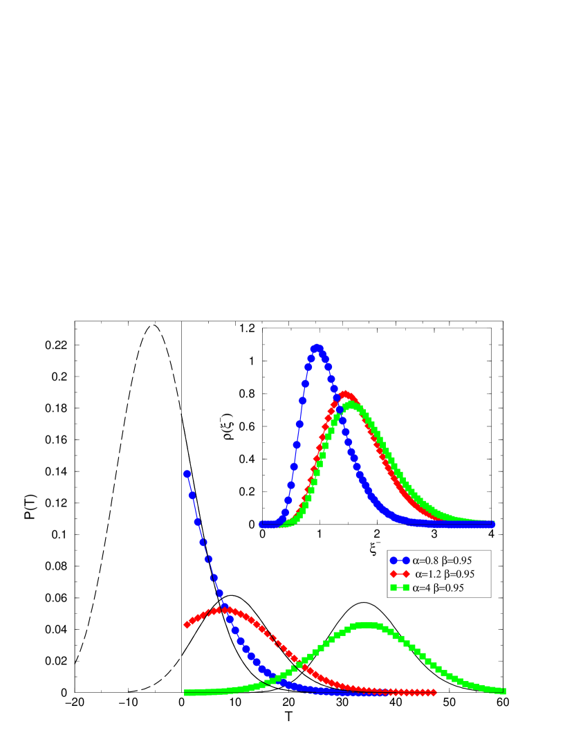
Figure 2: (Color online.) Interevent time distribution $P(T)$ for $\beta=0.95$ and $\alpha=0.8,1.2,$ and $4$. Lines with symbols are the numerical results and simple lines are the theoretical distribution (6) using $\xi^{-}=\langle\xi\rangle=1.17,1.66,1.765,$ respectively. After the maximum at $T_{max}$, $P(T)$ decays faster than exponentially to zero (only times $T>0$ have physical meaning). The inset shows the PDF of $\xi^{-}$ obtained numerically for the same parameters.

The existence of such a most probable interevent interval $T_{max}$ resembles results obtained in models presenting stochastic resonance stocres or coherence resonance pikovsky . However, this is not the case of our model since it has neither a periodic input signal nor a resonance behavior for different noise amplitudes. In fact, in our case $T_{max}$ varies with the control parameters $\alpha,\beta$, whereas a modified (constant in time) variance of ${\xi_{n}}$ is equivalent to a simple rescaling of the length scale and do not affect time scales. We would like to obtain now the dependence of $T_{max}$ on $\alpha,\beta$. A direct analysis through the theoretical distribution (6) is difficult due to its complicated expression and due to the lack of knowledge of the distribution of $\xi^{-}$, which also strongly depends on $\alpha,\beta$. Fortunately some intuition can be gained through simple approaches developed in what follows. Qualitatively, we notice that the existence of a most probable interevent time is a consequence of the reduction of the probability of short interevent times due to the increment of the barrier size after one extreme event. We expect thus that $T_{max}$ increases with $\alpha$ and that for $\alpha\leq 1$, $P(T)$ decays monotonically with $T$. These results are verified numerically in Fig. 3a,b. It is also interesting to note that the characteristic interevent time $T_{max}$ also shows up in the spectrum and autocorrelation function of the series $\{y_{n}\}$ and $\{q_{n}\}$.

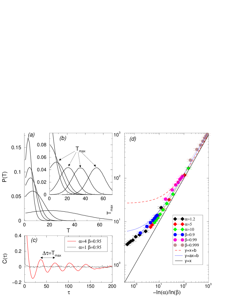
Figure 3: (Color online.) Numerically obtained interevent time distribution $P(T)$ for (a) $\alpha=1.2$ and $\beta=0.7,0.85,0.89,0.94,0.98$ (from left to right), and (b) for $\beta=0.95$ and $\alpha=0.8,1,1.2,2,4,10$ (from left to right). (c) Auto-correlation function of the series $y_{n}$. (d) Dependence of $T_{max}$ on the control parameters $\alpha,\beta$.

Consider now that $\xi_{n}$ assumes the constant value $\xi^{*}>0$. In this simple case the time between events is given by the time the barrier takes to decay to a value smaller than $\xi^{*}$: $q^{*}=\xi^{*}=\alpha\xi^{*}\beta^{T}\Rightarrow T=-\frac{\ln\alpha}{\ln\beta}$. Another simple approach is to consider that the next extreme event occurs when the barrier is at $q^{+}$ and the previous one occurred due to a value $\xi^{-}$, where the distributions of ($\xi^{-},q^{+}$) are unknown and depend on $\alpha,\beta$. We obtain in this case an interevent time $T$,

$$q^{+}=\alpha\xi^{-}\beta^{T}\Rightarrow T=-\frac{\ln\alpha}{\ln\beta}+\frac{\ln(q^{+})-\ln(\xi^{-})}{\ln(\beta)}\;.$$

On average $\xi^{-}>q^{+}$ and thus $T_{max}>-\frac{\ln(\alpha)}{\ln(\beta)}$. In both cases we see that $T_{max}$ depends explicitely on the ratio $-\frac{\ln(\alpha)}{\ln(\beta)}$. In Fig. 3d we plot numerical obtained values of $T_{max}$ against $-\frac{\ln(\alpha)}{\ln(\beta)}$. We notice that all points collapse approximately in a same curve that is indeed always above the diagonal and that good agreement is achieved by a linear fitting.

4 Efficiency of the model

The most relevant issue in the socio-economic context is how to minimize the number of extreme events, or how to optimize the efficiency of a protection strategy. The rate of extreme events $\rho(y)>0$ is the simplest and most natural measure of the costs due to extreme events and is thus used throughout this paper. For many situations it is a realistic measurement of the damage that occur due to the overpass of a threshold (e.g, obstruction of a street or of the power supply), where there is no difference between ”small” and ”large” extreme events. In other situations, more detailed accounts of the costs would make use of cost functions that depend (non-linearly) on $y$. Our model can be considered as a specific method which can be optimized by the choice of the control parameters $\alpha,\beta$.

The rate of extreme events $\rho(y>0)$ as a function of the control parameters is shown in Fig. 4. Since the barrier $q$ do not necessarily increase after one extreme event if $\alpha<1$, we notice again a qualitatively different behavior for $\alpha<1$ and $\alpha>1$. For a fixed $\beta$ and varying $\alpha$ (Fig. 4a) we notice that the number of extreme events decays drastically around $\alpha\approx 1$. On the other hand, by fixing $\alpha$ and varying $\beta$ (Fig. 4b) the number of extreme events goes much faster to zero when $\beta\rightarrow 1$ if $\alpha>1$.

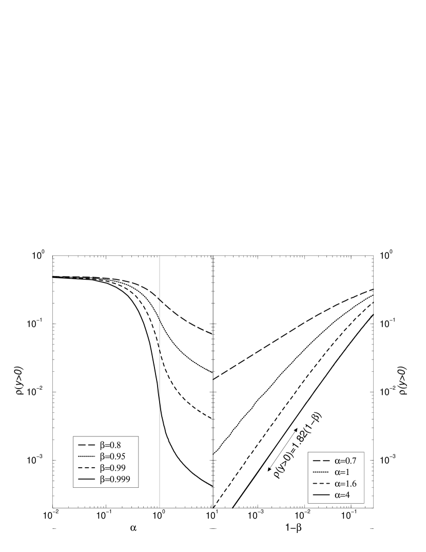
Figure 4: Extreme events rate $\rho(y>0)$ as a function of the control parameters $\alpha$ and $\beta$.

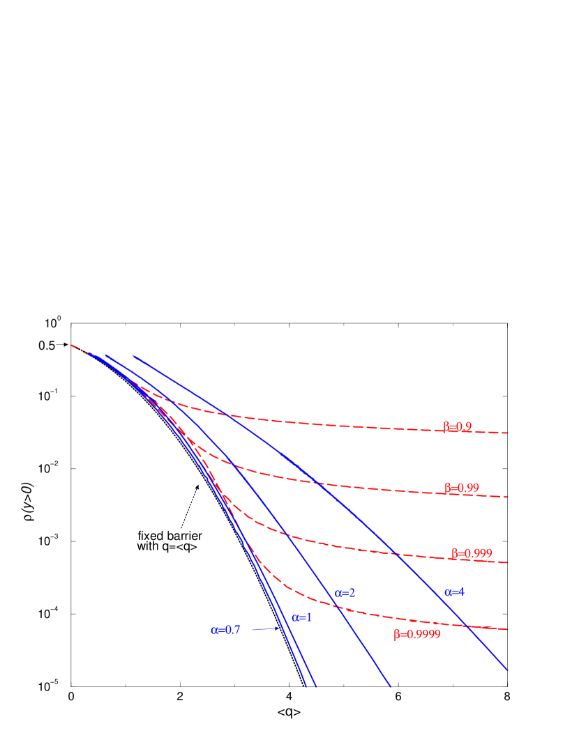
Figure 5: (Color online.) Extreme events rate $\rho(y>0)$ as a function of the mean barrier $\langle q\rangle$ (costs). Dashed lines are obtained by fixing the control parameter $\beta$ and varying $\alpha$, and continuous lines by fixing $\alpha$ and varying $\beta$. The dotted line at left correspond to a constant barrier in time $q_{t}=\langle q\rangle$.

It is quite natural that the number of extreme events is reduced when the control parameters increase. However, in real situations the increment of these parameters, or equivalently the increment of the barrier, is related to some costs that have to be taken into account when studying the efficiency of the model. Since the costs are usually increasing with the size of the barrier, we measure them by the mean value of the barriers $\langle q_{n}\rangle$. In Fig. 5 the rate of extreme events is shown against $\langle q\rangle$ for different values of the control parameters $\alpha,\beta$ and is compared with the result (dotted line) obtained when the barrier is maintained unchanged in time. As already suggested in Eq. (3), we notice that our moving threshold method is always less efficient than the constant barrier case. The limit of unchanged barrier is obtained in our model for $\alpha\rightarrow 0$ and $\beta\rightarrow 1$, when the most efficient results are obtained. By noting that the lines of constant $\alpha$ are approximately parallel to this limit, we realize that the relevant limit is $\beta\rightarrow 1$. Indeed, for any $\alpha\approx 1$ an efficient reduction of the number of extreme events is only possible by increasing $\beta$ towards one.

5 Non-stationarities

In the previous section we have seen that the model proposed in this paper to simulate the feedback reactions to extreme events is always less efficient than maintaining the size of the barrier constant in time, i.e., a non-reactive model. On the other hand, a clear advantage of reactive models is their ability to deal with non-stationarities in the time series. This is a specially important issue when considering extreme events since in many cases they are indeed originated from process presenting slow trends. Once more, these trends may be natural or consequence of human activities (e.g., change in land use, global warming).

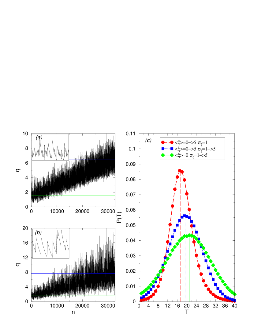
Figure 6: (Color online.) Time series of the barrier $q$ for $\alpha=1.2,\beta=0.95$ and: (a) linear increment in time of $\langle\xi\rangle$ with $\langle\xi\rangle^{f}=5$ and (b) linear increment in time of $\sigma_{\xi}$ with $\sigma^{f}_{\xi}=5$. The horizontal lines correspond to $\langle q\rangle$ at $n=0$ (bottom) and at $n=N=2^{15}$ (top). The insets show magnifications. (c) Numerically obtained interevent time distributions for $\alpha=2,\beta=0.95$ and different non-stationary scenarios (see legend). Vertical lines are located at the value of $T_{max}$. The stationary case for $\alpha=2,\beta=0.95$ is indistinguishable from the case where only $\sigma_{\xi}$ increases.

In order to explore how the model defined by Eq. (1) adapts to weak non-stationarities, we choose in this section the input time series $\{\xi_{n}\}$ to be a Gaussian delta correlated random variable with mean and variance changing linearly in time

$$\begin{array}[]{ll}\langle\xi\rangle=&\frac{\langle\xi\rangle^{f}}{N}n,\\ \sigma_{\xi}=&1+\frac{\sigma^{f}_{\xi}-1}{N}n,\\ \end{array}$$ (7)

where $N$ is the total observation time and $\langle\xi\rangle^{f},\sigma^{f}_{\xi}>0$ are constants. Note that increasing the value of $\langle\xi\rangle$ is not equivalent to a simple translation since the barrier is still limited to positive values $q>0$ and $\lim_{n\rightarrow\infty}\beta q^{n}=0$. In Fig. 6a,b we show that on large time scales the value of the barrier $q_{n}$ also increases linearly in time in both cases, i.e., when the mean or the variance increases in time. The linear increment of $\langle q\rangle$ increase also the fluctuations ($\sigma_{q}$) of the time series $\{q_{n}\}$ and $\{y_{n}\}$.

It is also interesting to compare the results for the interevent time distribution of non-stationary time series with those reported in Sec. 3 for the stationary case. When $\langle\xi_{n}\rangle$ increases (decreases) we note that the value $T_{max}$ of the peak of the interevent time distribution $P(T)$ slightly decreases (increases). This effect is quite natural since the probability of a large value of $\xi$ is constantly increasing (decreasing) when $\langle\xi\rangle$ increases (decreases). On the other hand, due to the linearity of Eqs. (1), a change of the variance $\sigma_{\xi}$ lead to a rescale of $q$ without changing the value of $T_{max}$. Both effects are verified numerically in Fig. (6)c.

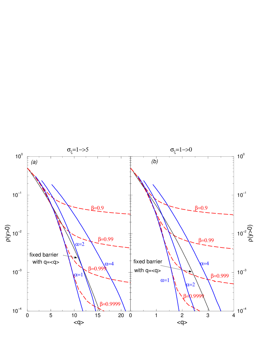
Figure 7: (Color online.) Extreme events rate $\rho(y>0)$ as a function of the mean barrier $\langle q\rangle$. Dashed lines are obtained by fixing the control parameter $\beta$ and varying $\alpha$, and continuous lines by fixing $\alpha$ and varying $\beta$. The dotted line correspond to a constant barrier in time $q_{t}=\langle q\rangle$. Two non-stationary situation are considered (a) $\sigma^{f}_{\xi}=5$ and (b) $\sigma^{f}_{\xi}=0$. $\langle\xi\rangle=0$ is constant for both cases.

Since the barrier increases proportionally to the size of the extreme event, we see that the time our model takes to adjust to non-stationarities is given by the interevent time $T$. When $T_{max}$ is much smaller than the total observation time, as considered here, the non-stationary effects can be considered small during this time interval. As a consequence of this fast adaptability of our model to the application of relations (7) we have that the dependence of the number of extreme events on the parameters $\alpha,\beta$ is qualitatively equivalent to the one reported in Sec. 4 for the stationary case. In order to obtain the efficiency we have to compare again the extreme events rate $\rho(y>0)$ with the mean barrier $\langle q\rangle$ (costs). However, now the value of $q$ is driven by changes of $\langle\xi\rangle$ (the value $\langle q\rangle$ reflects only the period of larger $\langle\xi\rangle$) showing that the efficiency analysis does not make sense in this case. More interesting is the case when the variance $\sigma_{\xi}$ changes in time and the mean value $\langle\xi\rangle$ is kept constant, shown in Fig. 7 for both increasing and decreasing $\sigma_{\xi}$. The comparison with the results obtained with constant barrier shows that with reasonable choice of parameters $\alpha,\beta$ the moving threshold model leads to a much more efficient result.

6 Conclusion

In summary, we have introduced a model to simulate human reactions or natural feedback response to extreme events. We have obtained that the sequence of extreme events occur with a certain periodicity, exclusively due to the human activity (natural feedback). Regarding the efficiency of the model, we have obtained that the best strategy in order to efficiently reduce the number of extreme events is to try to avoid the decrease of the protection barriers in the periods between extreme events. On the other hand, if slow non-stationarities are present in the phenomena, it is also useful to increase the usual protections to the value of the previous extreme event. The same conclusion is also expected for positively correlated sequences of events.

These results are obtained in a very simplified model that tries to isolate the influence of the human reactions to extreme events. In more realistic setups the properties discussed here may appear together with system-specific characteristics. In this sense, we can relate the characteristic interevent time observed in our model with the observed interepidemic interval between, e.g., smallpox epidemics bio2 . Direct association of realistic preventive schemes with the control parameters of our model lead to the estimation of the characteristic interevent time. For instance, in the example of floods in river we may estimate that barriers are reduced by $2\%$ every year and that after a flood they are increased by $20\%$ more than the highest water level. With these parameters and ignoring deviations of Gaussianity, we obtain through our model the reasonable estimation of a $53$ years period between floods.

References

- (1) S. Albeverio, V. Jentsch, H. Kantz (eds.), Extreme Events in Nature and Society, Springer, Berlin, 2005.
- (2) H. Kantz et al., Dynamical Interpretation of Extreme events: predictability and predictions, Chapter 4 of Ref. book .
- (3) The opposite effect, i.e., the influence of extreme events in human opinions, was considered in: Fortunato and Stauffer, Chapter 11 of Ref. book .
- (4) N. Pinter, Science 308 (2005) 207.
- (5) K. Glass and B.T. Grenfell, J. theor. Biol. 221 (2003) 121.
- (6) K. Shimazaki and T. Nakata, Geophys. Res. Lett. 7 (1980), 279.
- (7) J. Davidsen and H. G. Schuster, Phys. Rev. E 65 (2002), 026120.
- (8) L. Gammaitoni, P. Hänggi, P. Jung, F. Marchesoni, Rev. Mod. Phys. 70 (1998) 223.
- (9) E. G. Altmann and H. Kantz, Phys. Rev. E 71 (2005) 056106.
- (10) H.-J. Stöckmann, Quantum Chaos: An introduction, Cambridge University Press, Cambridge, 1999 (p. 93).
-
(11)
The following identity was used (see http://functions.wolfram.com/):
- (12) A. S. Pikovsky and J. Kurths, Phys. Rev. Lett., 78 (1997) 775.
- (13) C.J. Duncan, S.R. Duncan, S. Scott, J. theor. Biol. 183 (1996) 447.