Model of mobile agents for sexual interactions networks

Abstract

We present a novel model to simulate real social networks of complex interactions, based in a granular system of colliding particles (agents). The network is build by keeping track of the collisions and evolves in time with correlations which emerge due to the mobility of the agents. Therefore, statistical features are a consequence only of local collisions among its individual agents. Agent dynamics is realized by an event-driven algorithm of collisions where energy is gained as opposed to granular systems which have dissipation. The model reproduces empirical data from networks of sexual interactions, not previously obtained with other approaches.

1 Introduction

A social network is a set of people, each of whom is acquainted with some subset of the others. In such a network the nodes (or vertices) represent people joined by edges denoting acquaintance or collaboration. Empirical data of social networks include networks of scientific collaborationNewmanPNAS , of film actor collaborationsstrogatznat , friendship networksAmaral among some othersNewmanSIAM . One kind of social network is the network of sexual contactsnature93 ; Liljeros ; UK ; Latora , where connections link those persons (agents) that have had sexual contact with each other. The empirical investigation of such networks are of great interest because, e.g. the topological features of sexual partners distributions help to explain why persons can have the same number of sexual partners and yet being at distinct risk levels of contracting HIV Klovdahl .

The simplest way to characterize the influence of each individual on the network is through its degree $k$, the number of other persons to whom the individual is connected. Sexual contact networks are usually addressed as an example of scale-free networksLiljeros ; UK ; Latora ; barabasirev , because its property of having a tail in its degree distribution, which is well fitted by a power-law $P(k)\sim k^{-\gamma}$, with an exponent $\gamma$ between $2$ and $3$. However, another characteristic feature, not taken into account, is that the small $k$-region, comprehending the small-k values varies slowly with $k$, deviating from the power-law. Moreover, the size of the small-$k$ region also increases in time, yielding rather different distributions when considering the number of partners during a one year period or during the entire life, e.g. for entire-life sexual contacts, the degree distribution shows that at least half of the nodes have degree in the small-$k$ region nature93 ; Liljeros . A model predicting all these different distributions shapes for different time spans is of crucial interest, because the transmission of diseases occur during the growth mechanism of the network.

One of the main difficulties for validating a model of sexual interactions is that typical network studies of sexual contacts involve the circulation of surveys, or anonymous questionnaires, and only the number of sexual partners of each interviewed person is known, not being possible to obtain information about the entire network, in order to calculate degree correlations, closed paths (cycles), or average distance between nodes.

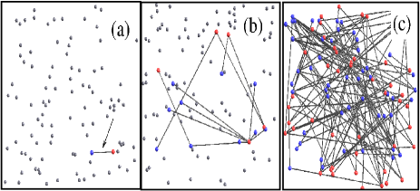
Figure 1: Snapshots of the growing network of collisions in a low-density gas with $N=100$, for (a) $n=0.02N$, (b) $n=0.15N$, (c) $n=N$. In the on-line version two colors represent the two sexual genders and larger symbols emphasize those which belong to the network (linked agents).

In this work we propose a model of mobile agents in two dimensions from which the network is build by keeping track of the collisions between agents, representing the interactions among them. In this way, the connections are a result not of some a priori knowledge about the network structure but of some local dynamics of the agents from which the complex networks emerge. Below, we show that this model is suitable to reproduce sexual contact networks with degree distribution evolving in time, and we validate the model using contact tracing studies from health laboratories, where the entire contact network is known. In this way, we are able to compare the number of cycles and average shortest path between nodes as well as compare the results with the ones obtained with Barabási-Albert scale-free networksAlbertScience , which are well-known models, accepted for sexual networksLiljeros ; UK ; Latora . We start in Sec. 2 by describing the model of mobile agents, and in Sec. 3 we apply it to reproduce the statistical features of empirical networks of sexual contacts. Discussion and conclusions are given in Sec. 4.

2 Model of mobile agents for sexual interactions

The model introduced below is a sort of a granular systemrefpoeschel , where $N$ particles with small diameter $d$ represent agents randomly distributed in a two-dimensional system of linear size $L\gg\sqrt{N}d$ (low density) and the basic ingredients are an increase of velocity when collisions produce sexual contacts, two genders for the agents (male and female), and $n/N$, the fraction of agents that belong to the network, which constitutes an implicit parameter for the resulting topology of the evolving the network.

The system has periodic boundary conditions and is initialized as follows: all agents have a randomly chosen gender, position and moving direction with the same velocity modulus $|\vec{v}_{0}|$. We mark one agent from which the network will be constructed. When the marked agent collides for the first time with another one of the opposite gender, the corresponding collision is taken as the first connection of our network and its colliding partner is marked as the second agent of the network (Fig. 1a). Through time, more and more collisions occur, increasing the size $n$ of the network (Fig. 1b and 1c) till eventually all the agents composing the system are connected.

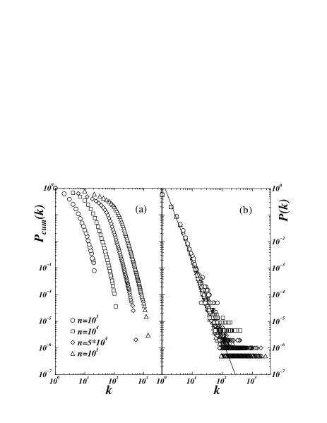
Figure 2: (a) Cumulative distribution $P_{cum}(k)$ of the number $k$ of partners among agents, when considering type-(i) and -(ii) interactions (see text) for $n=10^{3}$ (circles), $n=10^{4}$ (squares), $n=5\times 10^{4}$ (diamonds) and $n=10^{5}$ (triangles). For the same parameter values (b) shows a pure scale-free distribution, obtained when only type-(ii) interactions form links. The solid line indicates the slope $\gamma=3$ of the scale-free distribution. Here $\alpha=1$ and $N=320\times 320$.

Collisions between two agents take place whenever their distance is equal to their diameter and the collision process is based on an event-driven algorithm, i.e. the simulation progresses by means of a time ordered sequence of collision events and between collisions each agent follows a ballistic trajectoryRapaport . Since sexual interactions rely on the sociological observationLaumann that individuals with a larger number of partners are more likely to get new partners, we choose a collision rule where the velocity of each agent increases with the number $k$ of sexual partners. The larger the velocity one agent has the more likely it is to collide. Moreover, contrary to collision interactions where velocity direction is completely deterministicben-Avraham , here the moving directions after collisions are randomly selected, since in general, sexual interactions do not determine the direction towards which each agent will be moving afterwards. Therefore, momentum is not conserved.

Regarding these observations our collision rule for sexual interactions reads

$$\vec{v}(k_{i})=(k_{i}^{\alpha}+|\vec{v}_{0}(i)|)\vec{\omega},$$ (1)

where $k_{i}$ is the total number of sexual partners of agent $i$, exponent $\alpha$ is a real positive parameter, $\vec{\omega}=(\vec{e}_{x}\cos{\theta}+\vec{e}_{y}\sin{\theta})$ with $\theta$ a random angle and $\vec{e_{x}}$ and $\vec{e_{y}}$ are unit vectors. Collisions which do not correspond to sexual interactions only change the direction of motion.

Collisions corresponding to sexual interactions, i.e. with a velocity update as in Eq. (1), are the only ones which produce links, and occur in two possible situations: (i) between two agents which already belong to the network, i.e. between two sexually initiated agents and (ii) when one of such agents finds a non-connected (sexually non-initiated) agent. For simplicity, we do not take into account sexual interactions between two non-connected agents, and therefore our network is connected (see the discussion in Sec. 4).

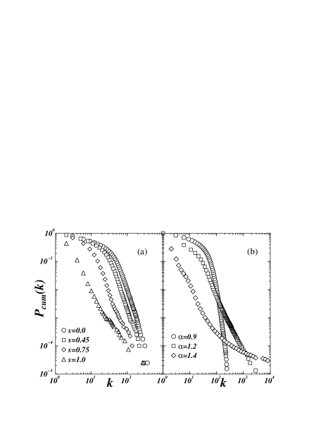
Figure 3: Cumulative distributions, when varying (a) a parameter $s$ of selectivity which interpolates between Figs.2a and 2b (see text) for $\alpha=1$ and (b) the exponent $\alpha$ in the update velocity rule, Eq. (1), for $s=0$. Here the same stage of growth is considered, namely $n=5\times 10^{4}=0.5N$.

When interactions of type (i) and (ii) occur, both the distribution tail and the small-$k$ region are observed, as shown by the cumulative distribution $P_{cum}(k)$ in Fig. 2a. Here, we use a system of $N=320\times 320$ agents with $\rho=0.02$, $\alpha=1$ and distributions are plotted for different stages of the network growth, namely $n=10^{3}$, $n=10^{4}$, $n=5\times 10^{4}$ and $n=10^{5}\sim N$. As one sees, the exponent of the power-law tail and the transition between the tail and the small-$k$ region increase during the growth process. These features appear due to the fact that at later stages most of the collisions occur between already connected agents. Consequently, the average number of partners increases as well.

If one considers only type-(ii) sexual contacts, the system reproduces a stationary scale-free network, as shown in Fig. 2b. In this case the average number of partners, defined aseames02 $\langle k\rangle=k_{min}(\gamma-1)/(\gamma-2)$ with $k_{min}$ the minimum number of partners, is always $2$ ($k_{min}=1$ and $\gamma=3$). As we show below, while empirical data of sexual contacts over large periods have distributions like the ones for regime (i)+(ii), data for shorter periods ($1-10$ years) are scale-free (only (ii)).

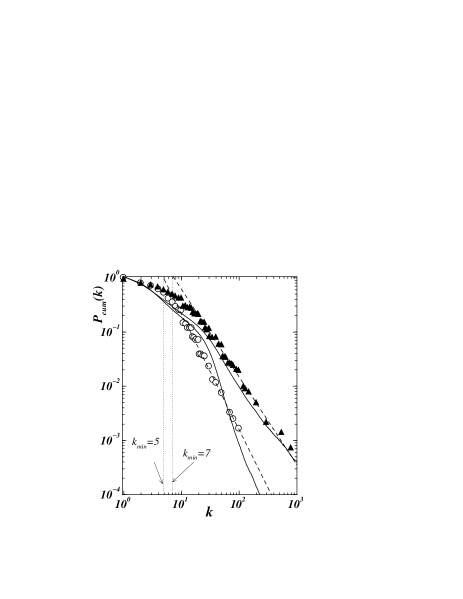
Figure 4: Cumulative distribution of sexual partners in a network of heterosexual contacts extracted from Ref. Liljeros , where male (triangles) and females (circles) distributions are plotted separately, with a total of $2810$ persons. Solid lines indicate the simulations when plotting the distributions at the same stage $n=0.2N$, starting with a population composed by $58\%$ of females and $42\%$ of males. Here $N=10^{5}$, $s=0$

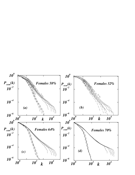
Figure 5: Distributions of sexual partners in a network of heterosexual contacts using different amounts of females: (a) $58\%$ as in Fig. 4, (b) $52\%$, (c) $64\%$ and (d) $70\%$. In each plot solid and dashed lines indicate the cumulative distributions of males and females respectively, for five different realizations. Clearly, the exponent of the power-law tail of the distributions decreases when the percentage of females or males increases (see dotted lines). Same conditions as in Fig. 4 were used.

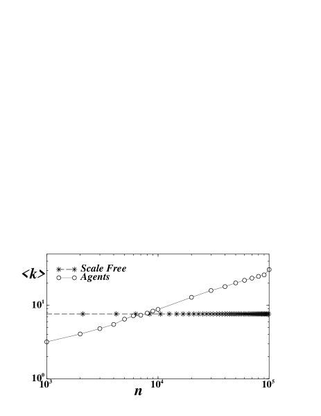
Figure 6: Comparing the average number of partners for scale-free networks (stars) and the agent model (circles). For the scale-free network $k_{min}=4$ and for agent model $N=520\times 520$, $s=0$.

With our model one can easily interpolate between both interaction regimes, (i)+(ii) and (ii), by introducing a parameter $s$ of ‘selectivity’, defined as the probability that sexual initiated agents in case of collision with another initiated agent, have no sexual contact. Physically, this selectivity accounts for the intrinsic ability that a node has to select from all its contacts (collisions) the ones which are sexual. These intrinsic abilities were already used in other contexts, e.g. as a new mechanism leading to scale-free networks in cases where the power-law degree distribution is neither related to dynamical properties nor to preferential attachmentCaldarelli . For $s=0$ one obtains the two regions illustrated in Fig. 2a, namely the small-$k$ region and the power-law tail, while for $s=1$ one obtains the pure scale-free topology illustrated in Fig. 2b. In Fig. 3a, we show the crossover between these two regimes.

The shape of the cumulative distributions is also sensible to the exponent $\alpha$ in the update velocity rule, Eq. (1), as shown in Fig. 3b. While for small values of $\alpha\lesssim 1$ one gets an exponential-like distribution, for $\alpha\gtrsim 1.4$ the distribution shows that a few nodes make most of the connections. Henceforth, we fix $\alpha=1.2$.

Having described the model of mobile agents we proceed in the next section of a specific application, i.e. modeling empirical networks of sexual contacts.

3 Reproducing networks of sexual contacts

In this Section we will show that, by properly choosing the parameter values in our model, one can reproduce real data distributions of sexual contact networks. In Fig. 4 the cumulative distributions of a real contact networkLiljeros are shown for females (circles) and males (triangles) separately, based on empirical data from $2810$ persons in a Swedish survey of sexual behavior. The solid lines in Fig. 4 indicate the simulated distributions. The simulated power-law tails have exponents $\gamma_{m}=2.4$ and $\gamma_{f}=4.0$ for males and females respectively, compared with the empirical data $\gamma_{m}=2.6\pm 0.3$ and $\gamma_{f}=3.1\pm 0.3$Liljeros . To stress that, while the power-law tails are also well fitted by distributions obtained with scale-free networks (dashed lines in Fig. 4), these distributions have a minimum number of connections (partners) of $k_{min}=5$ for females and $k_{min}=7$ for males, contrary to the real value $k_{min}=1$ also reproduced with our agent model. In fact, the model of mobile agents takes into account not only the power-law tail of these distributions, but also the small-$k$ region which comprehends the significant amount of individuals having only a few sexual partners ($k\gtrsim 1$).

Is important to note that in order to reproduce the difference in the exponents is necessary to have $58\%$ females and $42\%$ males, which is far from the expected difference among number of females and males in typical human populations, with ratios of females:males of the order of $1.1$. The difference in the exponents of the distributions tails for males and females separately, present in the data of sexual surveys, has generated much controversy and is often considered due to a bias either of sampling or honest reporting (see Ref. nature93 and references therein). The exponents $\gamma_{m}$ and $\gamma_{f}$ on a bipartite network are expected to be nearly the same when the percentage of males and females are similar, as shown in Fig. 5. In each plot five different realizations are shown for males (solid lines) and females (dashed lines). In Fig. 5a, we plot the results for the same conditions as in Fig. 4 ($58\%$ females and $42\%$ males). Taking the average of the five curves for each gender yields the curves shown in Fig. 4. Figures 5b-d show the distributions obtained for other percentages illustrating that when decreasing the difference in the ratio females:males difference in the exponents dissappear.

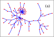
Figure 7: Sketch of two real sexual contact networks having (a) only heterosexual contacts ($N=82$ nodes and $L=84$ connections) and (b) homosexual contacts ($N=250$ nodes and $L=266$ connections). While in the homosexual network triangles and squares appear, in the heterosexual network triangles are absent (see Table 1).

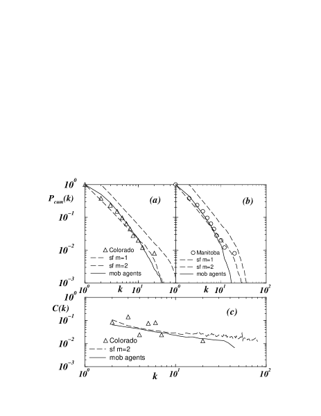
Figure 8: (a) Cumulative degree distribution of a homosexual contact networkcospring2 with $n=250$ (triangles). (b) Cumulative degree distribution of a heterosexual contact networkcospring1 with $n=82$ (triangles). Each case is compared with the average degree distribution over $20$ iterations, for the $BA$ scale-free model (dashed line) with $k_{min}=1$, and $k_{m}in=2$ and with our agent model (solid line) with $s=0.7$. (c) Cluster coefficient for the homosexual network empirical data (triangles), the agent model (solid line) and the $sf$ model $k_{min}=2$. The scale-free $k_{min}=1$ yields $C(k)=0$ (not shown).

	$N$	$L$	$T$	$Q$	$C$
Heterosexual	$82$	$84$	$0$	$2$	$0$
Homosexual .	$250$	$266$	$11$	$6$	$0.02980$
Heterosexual	$82$	$83.63$	$0$	$1.45$	$0$
(Agent Model)
Homosexual	$250$	$287.03$	$8.23$	$10.52$	$0.02302$
(Agent Model)
Heterosexual	$82$	$162$	$0$	$159.72$	$0$
(Scale-free)
Homosexual	$250$	$498$	$45.28$	$256.79$	$0.08170$
(Scale-free)

Table 1: Clustering coefficients and cycles in two real networks of sexual contacts (top), one where all contacts are heterosexual and another with homosexual contacts. In each case one indicates the values of the number $N$ of nodes, the number $L$ of connections, the number $T$ of triangles, the number $Q$ of squares and the average clustering coefficient $C$. The values of these quantities are also indicated for networks constructed with the agent model and for scale-free networks with $k_{min}=2$, note that for $k_{min}=1$, L=81 and L=249, respectively and there are not cycles.

A characteristic feature of our model is that the average number $\langle k\rangle$ of partners increases as the network grows, which is natural characteristic expected to occur in real sexual networks according to the observed differences in the shape of the degree distribution for yearly and entire-life reports of number of sexual partners Liljeros ; UK . This feature is not observed in scale-free networks, as illustrated in Fig. 6. Of course, that this growth also indicates non-stationary regimes, where $\langle k\rangle$ diverges with the network growth. In the next section we explain how to overcome this shortcoming.

We compare the model, with two empirical networks of sexual contacts. One network is obtained from an empirical data set, composed solely by heterosexual contacts among $n=82$ nodes, extracted at the Cadham Provincial Laboratory (Manitoba, Canada) and is a 6-month block data cospring1 between November 1997 and May 1998 (Figure 7a sketches this network). The other data set is the largest cluster with $n=250$ nodes in the records of a contact tracing study cospring2 , from 1985 to 1999, for HIV tests in Colorado Springs (USA), where most of the registered contacts were homosexual (see Figure 7b).

Figures 8(a)-(b) show the cumulative distribution of the number of sexual partners for each of the empirical networks. For both cases the agent model and scale-free networks with $k_{min}=1$ can reproduce the distribution of the number of partners. However, the agent model with $s=0.7$ reproduces, as well, the clustering coefficient distribution that we measure from the empirical network.

The clustering coefficient $C(i)$ of one agent is definedstrogatznat as the total number of triangular loops of connections passing through it divided by the total number of connections $k_{i}$. Averaging $C(i)$ over all nodes with $k_{i}$ neighbors yields the clustering coefficient distribution $C(k)$. While for the scale-free graph which better reproduces these empirical data, the clustering coefficient is zero, our agent model yields a distribution which resembles the one observed in the real network (Fig. 8c). This feature is due to the co-existence of a tree-like substructure and closed paths (see Figs. 7b).

For both heterosexual and homosexual networks of sexual contacts, the model of mobile agents reproduces other important statistical features, namely the average clustering coefficient $C$ and the number of loops of a given order. Table 1 indicates the number $T$ of triangles (loops composed by three edges), the number $Q$ of squares (loops with four edges) and the average clustering coefficients $C$ given bystrogatznat the average of $C(i)$ over the entire network.

When using the agent model with the same number $N$ of nodes as in the real networks we obtain similar results for $L$, $T$, $Q$ and $C$, as shown in Table 1 (middle), where values represent averages over samples of $100$ realizations. For the heterosexual network there are no triangles due to the bipartite nature of the network. At the bottom of Table 1 we also show the values obtained with scale-free networks, for both cases of one and two genders, whose minimum number of connections was chosen to be $k_{min}=2$, for which the clustering coefficient distributions are as close as possible from the distributions of the real networks. Clearly, the agent model not only yields clustering coefficient values much closer to the ones measured in the empirical data, but also does not show the formation of huge amounts of loops (triangles and squares), a feature of scale-free networks which is not observed in empirical data.

4 Discussion and conclusions

In this paper we presented a new model for networks of complex interactions, based on a granular system of mobile agents whose collision dynamics is governed by an efficient event-driven algorithm and generate the links (contacts) between agents. As a specific application, we showed that the dynamical rules for interactions in sexual networks can be written as a velocity update rule which is a function of a power $\alpha$ of the previous contacts of each colliding agent. For suitable values of $\alpha$ and selectivity $s$, the model not only reproduces empirical data of networks of sexual contacts but also generates networks with similar topological features as the real ones, a fact that is not observed when using standard scale-free networks of static nodes.

Furthermore, our model predicts that the growth mechanism of sexual networks is not purely scale-free, due to interactions among internal agents, having a mean number of partners which increases in time. This should influence the predictions from models of spreading of infectionseames02 . Our agent model offers a realistic approach to study the emergence of complex networks of interactions in real systems, using only local information for each agent, and may be well suited to study networks in sociophysics, biophysics and chemical reactions, where interactions depend on specific local dynamical behavior of the elementary agents composing the network.

While given promising results the model may be improved in two particular aspects. First, it should enable the convergence towards a stationary regime with a growth process starting with all possible collisions instead of one particular agents from which the network is constructed. Second, the dependence of the above results on the velocity rule in Eq. (1) should be studied in detail, namely for the case of constant velocity ($\alpha=0$). Preliminary results have shown that the stationary regime is easily obtained with the model above by introducing a simple aging scheme, while by varying the parameter $\alpha$ one is able to reproduce other non-trivial degree distributions. Moreover, we introduced the selectivity parameter $s$ to select from all possibles social interactions (collisions) the ones which are of sexual nature. Without introducing this selectivity, the model of mobile agents is able to reproduce other social networks of acquaintances. These and other questions will be addressed elsewherenew .

References

- (1) M.E.J. Newman, Proc. Natl. Acad. Sci. 98, 404 (2001).
- (2) D.J. Watts and S.H. Strogatz, Nature 393, 440 (1998).
- (3) L.A.N. Amaral, A. Scala, M. Barthéĺemy, and H.E. Stanley (2000), PNAS 10, 21.
- (4) M.E.J. Newman, The structure and function of complex networks, SIAM Rev. 45, 167 (2003).
- (5) M. Morris, Nature 365, 437 (1993).
- (6) F. Liljeros, C.R. Edling, L.A.N. Amaral and H.E. Stanley, Nature 411, 907 (2001).
- (7) A. Schneeberger et al, Sex. Trans. Dis. 31, 380 (2004).
- (8) V. Latora, M. Marchiori, A. Nyamba and S. Musmeci, submitted to Preventive Medicine.
- (9) A.S. Klovdahl, Soc. Sci. Med. 28, 25 (2001).
- (10) R. Albert and A.-L. Barabasi, Rev. Mod. Phys. 74, 47 (2002).
- (11) A.L. Barabási, R, Albert, Science 286, 509 (1999).
- (12) T. Pöschel and S. Luding, Granular Gases, (Lecture Notes in Physics, 564, Springer-Verlag, 2001)
- (13) D.C. Rapaport, The Art of molecular dynamics simulation, (Cambridge University Press, Cambridge, 1995).
- (14) E.O. Laumann, J.H.Gagnon, R.T Michaels, Organization of Sexuality, (University of Chicago Press, 1994).
- (15) D. ben-Avraham, E. Ben-Naim, K. Lindenberg, A. Rosas, Phys. Rev. E 68, 050103 (2003).
- (16) K.T.D. Eames and M.J. Keeling, Proc. Nat. Ac. Sci. 99, 13330 (2002).
- (17) G. Caldarelli, A. Capocci, P. De Los Rios, M.A. Muñoz, Phys. Rev. Lett. 89, 258702 (2002).
- (18) J.J. Potterat, L. Phillips-Plummer, S.Q. Muth, R.B. Rothenberg, D.E. Woodhouse, T.S. Maldonado-Long, H.P. Zimmerman, J.B. Muth, Sex. Transm. Infect. 78, i159 (2002).
- (19) J.L. Wylie and A. Jolly, Sex. Transm. Dis. 28, 14 (2001).
- (20) M.C. González, P.G. Lind and H.J. Herrmann, in preparation, 2005.