Supermodes of photonic crystal CCWs and multimode bistable switchings with uniform thresholds

Abstract

Photonic crystal (PC) coupled cavity waveguides (CCWs) with completely separated eigenfrequencies (or supermodes) are investigated. Using a coupled mode theory, the properties of the supermodes, such as the electric field profiles, the eigenfrequencies (including the central frequencies and corresponding linewidths), and the quality factors (Qs) are expressed in very simple formulas, and these results agree well with those of “exact” numerical method. We also discuss the great differences between the supermodes and continuous modes, which are described by tight binding (TB) theory. Then, the properties of supermodes are used to investigate their potential applications in multichannel (covering the whole C-band) bistable switchings, and bistable loops are obtained numerically. We also predict and verify that all the thresholds are uniform inherently.

I Introduction

Photonic crystal (PC) pc:Eya87 ; pc:John87 coupled cavity waveguides (CCWs) ccow:ol ; ccow:prl , which are formed by series of coupled point defects in otherwise perfect PCs, have been investigated intensively using tight binding (TB) theory in the last several years ccow:shaya:oe ; ccow:shaya:preshg ; ccow:shaya:pre02 ; ccow:jqe ; ccow:JstQE , and the propagation mechanism of hopping between neighboring cavities has been clearly understood ccow:hop . Generally speaking, a periodic CCW possesses a continuous transmission band of $\Omega_{0}(1-\Delta\alpha/2+|\kappa|,1-\Delta\alpha/2+|\kappa|)$, where $\Omega_{0}$ is the eigenfrequency of an individual cavity and $\kappa$, $\Delta\alpha$ are two related overlap integrals ccow:ol ; ccow:prl . For convenience, the modes of the continuous band derived from TB theory are called TB-modes in this paper. Many potential applications, such as broadband dropping ccow:banddrop , broadband splitting ccow:spliter:apl ; ccow:spliter:apl03 , broadband optical switching and limiting ccow:ob:conti ; ccow:OL:conti , and ultrashort pulse transmission ccow:ultrashort are all based on the continuous transmission bands (TB-modes).

In practice, however, the number of the cavity $N$ is finite, and Born-von Karman periodic condition is used ccow:shaya:oe ; ccow:JstQE and $N$ discrete modes are obtained, which satisfy the dispersion relation of ccow:shaya:oe ; ccow:JstQE :

$$\omega(k_{m})=\Omega_{0}\left[1-\Delta\alpha/2+\kappa\cos(k_{m}R)\right]$$ (1)

$$\mbox{with }k_{m}=2m\pi/L,\quad m=0,\cdots,N-1$$

Where $R$ is the distance between two neighboring cavities, and $L$ is the total length of the system. When the coupling strength between the cavities are designed carefully, and some criteria are satisfiedccow:12D , a quasi-flat spectrum with $N$ small dips formed by the $N$ discrete modes may be obtainedccow:12D . Actually, the broadband operations mentioned above ccow:banddrop ; ccow:spliter:apl ; ccow:spliter:apl03 ; ccow:ob:conti ; ccow:OL:conti are all realized using the quasi-flat transmission band.

Figure 1: One dimensional photonic crystal CCW structure considered in this paper. The individual cavity of $C$ is represented by $C=\bar{a}babcbab\bar{a}$. Where $a$, $b$ and $c$ are three different kinds of medium layers with refractive indexes of $n_{a}$, $n_{b}$ and $n_{c}$, and physical thicknesses of $\lambda_{0}/(4n_{a})$, $\lambda_{0}/(4n_{b})$ and $\lambda_{0}/(2n_{c})$, respectively. The layer $\bar{a}$ is the same as layer $a$ except that the thickness is $a/2$. $\lambda_{0}$ is a reference wavelength.

On the other hand, one can also design a $N$-cavity CCW to make the $N$ modes separated completelyccow:12D , (these separated modes are called supermodes in this paper and the reasons are given below), rather than to form a quasi-flat band. We find that the predictions of TB theory become inexact (as shown below) in this case. Although the supermodes of a $N$-cavity system have been noticed earlyccow:12D , the properties of them are not investigated intensively (such as the mode profiles and linewidths of each supermodes), which prevents them from wide application.

According to the criterion developed in Ref. ccow:12D , one dimensional (1D) CCW with discrete supermodes is designed, as shown in Fig. 1. Although some numerical methods, such as the finite difference time domain method (FDTD) fdtd:taflove , transfer matrix tmm:linear ; ccow:tmm can be used to extract the properties we expected, we prefer to understand them from the viewpoint of physics and express them in analysis and simple formulas.

In this paper, a general coupled mode theory is presented to analysis the supermodes of $N$-cavity CCW systems, as shown in Fig. 1. The eigenfrequencies, including both the central frequencies and the corresponding linewidths (and also the quality factors), as well as the mode profiles of the supermodes are obtained, and agree well with “exact” numerical results (obtained using standard transfer matrix method). Subsequently, these properties of supermodes are used directly to design a potential application of multichannel bistable switchings in the whole C-band. Using the results of coupled mode theory, we prove that the thresholds of the multichannel switchings are low and uniform when Kerr media are carefully introduced into the cavities.

II Coupled mode theory analysis of supermodes

In the coupled mode theory presented in this paper, the electric field $\mathbf{E}_{\omega}(\mathbf{r})$ of the entire coupled cavity system is expressed as a linear superposition of the modes of the $N$ cavities:

$$\mathbf{E}_{\omega}(\mathbf{r})=\sum_{n=1}^{N}A_{n}\mathbf{E}_{\Omega}(\mathbf{r}-nR\mathbf{e}_{z})$$ (2)

where $A_{n}$ $(n=1,\cdots,N)$ are complex coefficients that determine the relative phase and amplitude of the cavities. $\mathbf{E}_{\omega}$ and $\mathbf{E}_{\Omega}(\mathbf{r}-nR\mathbf{e}_{z})$ are the fields of the entire coupled system and those of individual cavities centered at $nR\mathbf{e}_{z}$ respectively. $\mathbf{e}_{z}$ is the direction of the cavities being aligned. $\omega$ and $\Omega$ are the allowed frequency of the coupled system (is unknown now) and the frequency of an individual cavity (is already known). We normalize $\mathbf{E}_{\Omega}(\mathbf{r})$ to be unity according to $\int\epsilon^{0}(\mathbf{r})\mathbf{E}(\mathbf{r})\cdot\mathbf{E}(\mathbf{r})=1$, with $\epsilon^{0}(\mathbf{r})$ the dielectric function of an individual cavity. Eq. (2) is very similar to the linear superposition field used in TB theory, which reads ccow:ol ; ccow:prl :

$$\mathbf{E}_{K}(\mathbf{r})=\sum_{n=1}^{\infty}B_{n}\mathbf{E}_{\Omega}(\mathbf{r}-nR\mathbf{e}_{z})$$ (3)

where the superposition coefficients are $B_{n}=E_{0}\exp(-inKR)$. However, one may find great differences between them. In TB theory (Eq.(3)), the superposition coefficients are $B_{n}=E_{0}\exp(-inKR)$, which have the same modulars of $|E_{0}|$ for all the cases of $n$ from $1$ to $N$, and the relative phases between them are also determined. However, in Eq.(2), the coefficients of $A_{n}$ are arbitrary complexes, and the amplitudes and phases of them may be greatly different for various of $n$. This is one of the most important differences between supermodes and TB-modes.

Substituting Eq.(2) into the simplified form of Maxwell’s equations of:

$$\nabla\times\nabla\times\mathbf{E}=\epsilon(\mathbf{r})\frac{\omega_{0}^{2}}{c^{2}}\mathbf{E}$$ (4)

Then, we operate both sides of the resulting equation from left using the operator of $\int d\!\mathbf{r}\mathbf{E}(\mathbf{r}-mR\mathbf{e}_{z})\cdot$, one can obtain a group of coupled equations:

$$A_{m}+\sum_{m\neq n=1}^{N}C_{mn}A_{n}=0$$ (5)

where the coefficients $C_{mn}$ are defined as

$$C_{mn}=\frac{\Omega^{2}\beta_{mn}-\omega^{2}\alpha_{mn}}{\Omega^{2}-(1+\Delta\alpha_{m})\omega^{2}}$$ (6)

$$\beta_{mn}=\int d\,\mathbf{r}\epsilon(\mathbf{r}-nR\mathbf{e}_{z})\mathbf{E}(\mathbf{r}-mR\mathbf{e}_{z})\cdot\mathbf{E}(\mathbf{r}-nR\mathbf{e}_{z})$$ (7)

$$\alpha_{mn}=\int d\,\mathbf{r}\epsilon(\mathbf{r})\mathbf{E}(\mathbf{r}-mR\mathbf{e}_{z})\cdot\mathbf{E}(\mathbf{r}-nR\mathbf{e}_{z})$$ (8)

$$\Delta\alpha_{m}=\int d\,\mathbf{r}\Delta\epsilon\mathbf{E}(\mathbf{r}-mR\mathbf{e}_{z})\cdot\mathbf{E}(\mathbf{r}-mR\mathbf{e}_{z})$$ (9)

$$(\mathrm{with\ }\Delta\epsilon_{m}(r)=\epsilon(\mathbf{r})-\epsilon(\mathbf{r}-mR\mathbf{r}))$$

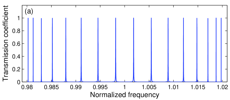
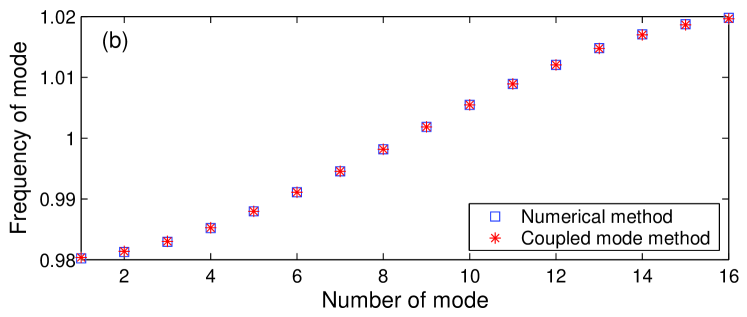
Figure 2: Comparison of the eigenfrequencies derived from the coupled mode theory and from numerical method for the structure of Fig. 1. The refractive indexes are $n_{a}=2$, $n_{b}=1$ and $n_{c}=2$ respectively. Number of cavities is $N=16$. (a) Transmission spectrum calculated using one dimensional transfer matrix method. (b) Comparison of the central frequencies of numerical results (Fig. 2(a)) with those derived from Eq. (15) with parameters of $\alpha=0.00499$, $\beta=-0.01497$ and $\Delta\alpha=0$ (See text for details). (c) Comparison the linewidths and quality factors of the supermodes derived from transfer matrix method (Fig. 2(a)) and coupled mode theory (Eq. (17)) with the parameter of $Q_{0}=2.6347\times 10^{4}$.

Eq. (5) is very similar to the governing equations of coupled waveguide arrays book:yariv , or phase-locked injection laser arrays cmt:apl ; cmt:JQE ; cmt:locklaser:ol , where, the solutions are called supermodes of the waveguide (or laser) arrays. Similarly, we name the solutions of Eq.(5) as the supermodes of the CCW. Generally, Eq. (5) can not be solved in closed form, however, it can be simplified and solved for some very special cases. For example, when only the nearest neighboring coupling are considered and the cavities are uniformly spaced. Then the coefficients are simplified to

$$C_{mn}=\frac{\Omega^{2}\beta-\omega^{2}\alpha}{\Omega^{2}-(1+\Delta\alpha)\omega^{2}}=\left\{\begin{array}[]{ll}C,&\hbox{$n=m\pm 1$;}\\ 0,&\hbox{others.}\\ \end{array}\right.$$ (10)

Here, we have used the relations of $\beta_{m,m\pm 1}=\beta$, $\alpha_{m,m\pm 1}=\alpha$ and $\Delta\alpha_{m}=\Delta\alpha$.

Then, using the same method as used in Ref.book:yariv ; cmt:apl ; cmt:JQE ; cmt:locklaser:ol and proper boundary conditions, one obtain the solutions of the Eq. (5). Generally, there’re $N$ solutions (supermodes) for a $N$-cavity CCW system. For the $L$th supermode, the linear superposition coefficients $A^{L}_{n}$ and $C^{L}$, respectively, are:

$$A_{n}^{L} = A^{L}\sin(n\theta^{L}),\quad n=1,\cdots,N$$ (11)

$$C^{L} = -\frac{1}{2\cos(\theta^{L})}$$ (12)

$$\theta^{L} = \frac{L\pi}{N+1},\quad L=1,\cdots,N$$ (13)

Where $A^{L}$ is a constant and is determined from the normalization condition of

$$\int d\mathbf{r}\epsilon(\mathbf{r})\left[\sum_{n=1}^{N}A_{n}\mathbf{E}_{\Omega}(\mathbf{r}-n\mathbf{e}_{z})\right]\cdot\left[\sum_{n=1}^{N}A_{n}\mathbf{E}_{\Omega}(\mathbf{r}-n\mathbf{e}_{z})\right]=1$$ (14)

After a simple algebra process and using the normalization condition of the individual cavity modes, one can obtain the constant of $A^{L}$ is $A^{L}=\sqrt{2/(N+1)}$, which is independent of the mode number of $L$.

According to Eq. (6) and Eq. (13), one can obtain the $N$ eigenfrequencies of the supermodes:

$$\omega^{L}=\Omega\sqrt{\frac{C^{L}-\beta}{C^{L}-\alpha+C^{L}\Delta\alpha}}\quad L=1,2,\cdots,N$$ (15)

Eq. (5) and Eq. (15) are the main results of the coupled mode theory discussed above. We want to point out that in Eq. (12), $C^{L}$ tends to infinite when $\theta^{L}=m\pi+\pi/2$ ($m$ is an integer). For example, when $N=5$ and $L=3$. However, this does not mean that the coupled mode theory is invalid in this case. Because the parameter of $C^{L}$ is a function of frequency of the supermode, $\alpha$ and $\beta$ (see Eq. (6)), but not an physical quality. The values of physical qualities of $A^{L}_{n}$ (Eq.(11)) and $\omega^{L}$ (Eq. (15)) are both finite and correct when compared with numerical results.

Actually, the method shown above is not new, and it has been considered in Ref. ccow:prl for the special cases of $N=2$ and $3$. When $N=2$, one can derive from Eq. (13) that $C^{1,2}=\mp 1$, and then from Eq. (15), one can obtain the frequencies of the supermodes and the superposition coefficients:

$$\omega^{1,2}=\Omega\sqrt{\frac{1\pm\beta}{1+\Delta\alpha\pm\alpha}},\quad A_{1,2}^{1}=\frac{1}{\sqrt{2}},\quad A_{1,2}^{2}=\pm\frac{1}{\sqrt{2}}$$ (16)

Clearly, the superposition coefficients and the corresponding frequencies in Eq. (16) are the same as the results of Eq. (2) in Ref. ccow:prl . Similarly, one also can calculate the frequencies and fields for the case of $N=3$, which are also the same as the results in Ref. ccow:prl . (In Eq. (3) of Ref. ccow:prl , the $\Delta\alpha$ is regarded as negligible small).

In order to show the power of the coupled mode theory discussed above, we consider a one dimensional CCW with a large number of cavities (i.e., $N=16$), as shown in Fig. 1. Using the standard transfer matrix method (TMM) tmm:linear , one can easily obtain the transmission spectrum, as shown in Fig. 2(a). Using Eq. (15), (12) and (13), one also can calculate the $16$ eigenfrequencies, and the results are shown in Fig. 2(b). Clearly, the theoretical results agree well with the numerical results. Here, the parameters are set to be $\alpha=0.00499$, $\beta=-0.01497$ and $\Delta\alpha=0$, which are obtained according to the following two steps: Firstly, we numerically obtain the two eigenfrequencies of $(\omega^{1,2}/\Omega_{0})=0.990017,1.009983$ for the case of $N=2$. Secondly using Eq. (16), we calculate the above parameters of $\alpha$, $\beta$. Here we assumed that $\Delta\alpha$ is negligible compared to $\alpha$ and $\beta$. On the contrary, when the values of $\alpha$, $\beta$, $\Delta\alpha$ and $k_{m}$ are substituted into Eq. (1), much larger errors of $\omega(k_{m})$ from the numerical results are found. Therefore, the coupled mode theory gives more exact results than the TB theory in the case of discrete supermodes.

The quality factors ($Q$’s) of the supermodes can also be derived from the results of coupled mode analysis. The $Q$’s of the $L$th supermode is defined as $Q^{L}=\omega^{L}W^{L}/\Delta W^{L}$, where $W^{L}=\frac{1}{2}\int_{V}d\mathbf{r}\mathbf{E}\cdot\mathbf{D}$ is the total energy stored in the coupled cavity system of the $L$th supermode, and $\Delta W^{L}=-dW^{L}/dt$ is the energy dissipated. According to the normalization condition of Eq. (14), one can easily find that the total energy of all the $N$ supermodes are the same, i.e, $W^{L}=W_{0}$. For the CCWs composed of lossless media, the dissipation of energy of the $N$ supermodes are all due to the coupling out of the system through the $1st$ and $N$th cavities. Therefore, the energy dissipation of $\Delta W^{L}$ is proportional to the energy stored in the first and last cavities, i.e., $\Delta W^{L}=\Delta W_{0}\sin^{2}(\theta^{L})$. Here, we have used the results of Eq. (11). Then, one can find the quality factor $Q^{L}$ of the $L$th supermode:

$$Q^{L}=\omega^{L}\frac{W^{L}}{\Delta W^{L}}=\omega^{L}\frac{W_{0}}{\Delta W_{0}\sin^{2}(\theta^{L})}\approx\frac{Q_{0}}{\sin^{2}(\theta^{L})}$$ (17)

Here, $Q_{0}=\Omega_{0}W_{0}/\Delta W$, and we have used the the fact of $\omega^{L}\approx\Omega_{0}$. The results of Eq. (17) have been shown in Fig. 2(c) with the parameter $Q_{0}=2.6347\times 10^{4}$.

On the other hand, we can also derive the $Q^{L}$ by finding the values of $Q^{L}=\omega^{L}/\Delta\omega_{fwhm}^{L}$ from the numerical results (Fig. 2(a)), where $\Delta\omega_{fwhm}^{L}$ is the full width at half maximum of the $L$th supermodes. The results are also shown in Fig. 2(c), and they agree well with the results of Eq. (17).

Fig. 3 shows the field profiles of the first half supermodes of $\omega^{1,\cdots,8}$. For the case of clarity, the modes of $\omega^{9,\cdots,16}$, which are very similar to the modes of $\omega^{8,7,\cdots,1}$ respectively, are not shown. Clearly, the results of coupled mode theory of Eq. (13) are agree well with those of the transfer matrix method. The amplitudes of individual cavities of the $L$th supermodes lie on an envelope function of $\sin(\frac{xL\pi}{N+1})$. Therefore, the amplitude of some cavity modes may be tend to zero, while others reach to maxima. In the TB model, however, the amplitude of all the cavity modes are the same.

From the discussion above, one can find that the coupled mode theory presented above describes the main characteristics of the supermodes very well, provided that the parameters of $\alpha$, $\beta$ and $Q_{0}$ are given. The supermode states of a CCW are very different with the states of TB-modes, which are described by the tight binding theoryccow:ol ; ccow:prl . For the TB-modes, the transmission band is determined by Eq. (1), while in the supermodes, the central frequencies are determined by Eq. (15). In the TB modes, the localizations in each cavities are the same, while in the supermodes, the localizations change greatly according to a simple sine function. In the next section, one of the possible applications of supermodes of multi-channel bistable switchings is proposed and analyzed using the results of coupled mode theory given above.

Figure 3: (Color online) The electric field profiles of supermodes calculated using transfer matrix method (blue lines) and the envelope of superposition coefficients (red lines with circles) shown in Eq. (11). The distribution of the refractive index is also shown for clarity.

Figure 4: (Color online) (a) Bistable switching loops and the thresholds of the $16$-channel switchings. (a) Switching loops of $\omega_{in}^{1,\cdots,8}$, and those of $\omega_{in}^{9,\cdots,16}$ are not shown for clarity, which are similar to $\omega_{in}^{8,\cdots,1}$. Normalized unit of light intensity of $n_{2}I$ is used with $n_{2}$ the Kerr nonlinear coefficient and $I$ the light intensity. (b) the thresholds of the $16$-channel switchings.

III Multi-channel bistable switchings with uniform thresholds

One of the potential applications of the supermodes is multichannel optical bistable (OB) switching, which is a key component in all optical information systems. The OB switching have been widely investigated in photonic crystals with Kerr defects ccow:ob:conti ; ob:clx:oc02 ; ob:side ; ob:dirct ; ccow:ob:discr , of which the refractive index changes with local light intensity. i.e., $n=n_{0}+n_{2}I$ with $n_{0}$ the linear refractive, $n_{2}$ the nonlinear Kerr coefficient and $I$ the local light intensity. However, most of the researches are focused on a single frequency operation ob:clx:oc02 ; ob:side ; ob:dirct . In a wavelength division multiplexer (WDM) system, there’re always need a multi-channel switching for all the working channels. We find that the supermodes of CCWs are very suitable for this function ccow:ob:discr . As an example, we investigate the systems of $16$-cavity CCW structures shown in Fig. 1.

According to the OB switching theory, the shift of the eigenfrequencies with the changes of the dielectric constants of the cavities is a key factor for OB operation. Using the perturbation theory pertub:prb2002 , one can find the shifts of eigenfrequencies of supermodes with the change of dielectric constant $\Delta\epsilon(\mathbf{r})$:

$$\Delta\omega^{L}=-\frac{\omega^{L}}{2}\frac{\int\Delta\epsilon(\mathbf{r})|\mathbf{E}_{\omega^{L}}(\mathbf{r})|^{2}}{\int\epsilon(\mathbf{r})|\mathbf{E}_{\omega^{L}}(\mathbf{r})|^{2}}$$ (18)

where $\mathbf{E}=\sum A_{n}\mathbf{E}(\mathbf{r}-n\mathbf{e}_{z})$ is the electric fields of supermodes of the unperturbed CCW.

When only the $1$st and $N$th cavities are perturbed by the same amount of $\Delta\epsilon$, then using the relation of Eq. (11), (14) and (18), one can derive that

$$\Delta\omega^{L}=-\frac{\omega^{L}}{2}\int_{C_{1},C_{N}}\Delta\epsilon|\mathbf{E}_{\omega^{L}}(\mathbf{r})|^{2}d\mathbf{r}=\Delta\omega_{0}|\sin(\theta^{L})|^{2}$$ (19)

Where, $\Delta\omega_{0}=-[\omega^{L}\Delta\epsilon/(N+1)]\int_{v}d\!\mathbf{r}|\mathbf{E}_{\Omega^{L}}(\mathbf{r})+\mathbf{E}_{\Omega^{L}}(\mathbf{r}-NR\mathbf{e}_{z})|^{2}$. On the other hand, according to Eq. (17), we find that the FWHMs of the supermodes are $\omega^{L}_{fwhm}=(\omega^{L}/Q_{0})\sin^{2}(\theta^{L})$. Therefore, the shifts of the frequencies are proportional to their FWHMs respectively, i.e., $\Delta\omega^{L}=(\Delta\omega_{0}Q_{0}/\Omega_{0})\omega^{L}_{fwhm}$. When the incident frequencies $\omega_{in}^{L}$ of the bistable switchings are tuned from the central frequencies according to $\omega_{in}^{L}=\omega^{L}-y\omega_{fwhm}^{L}$, the thresholds of the multi-channel bistable switching are expected to be uniform.

Using the nonlinear transfer matrix method ntmm:apl92 , and setting $y=2$, we obtain the bistable switching loops, and the results are shown in Fig. 4. In Fig. 4 we have used the normalized intensity of $n_{2}I$ ccow:ob:conti . We can see that the thresholds of the switchings are almost the same. Except for the $1$st and $16$th channel (In practice, the $1$st and $N$th channels may be tuned slightly in order to switch them with approximately the same thresholds as other channels), the maximum of the thresholds is $4.8\times 10^{-6}$ (the channel of $\omega_{in}^{15}$) and the minimum is $4.5\times 10^{-6}$ (the channel of $\omega_{in}^{8}$), and the relative difference is about $6\%$.

When the thicknesses of $a$, $b$ layers are $193.8nm$ and $387.5nm$ respectively, the central frequency of $\lambda_{0}$ is at about $1.55\mu m$, and the multi-channel frequencies cover the C-band of optical fiber communication entirely. For a Kerr nonlinear coefficient of $n_{2}=2\times 10^{-13}cm^{2}/W$ (a value achievable in many nearly instantaneous nonlinear materials), the thresholds are about $4.6\times 10^{-6}W/cm^{2}$, which is much smaller than those of the switchings studied before ccow:ob:conti ; ob:clx:oc02 .

IV Conclusion

In summary, we have analyzed the supermodes of CCW systems, which are different from the TB-modes and are also important operation states of CCWs. Using the coupled mode theory, the eigenfrequencies, including the centers and the FWHMs, quality factors, and mode profiles of the supermodes are formulated in very simple forms. And they agree well with exact numerical results. We also discussed the great difference of the supermodes with the quasiflat TB-modes. We investigated one of the potential applications of the supermodes, which is a $16$-channel bistable switching with uniform thresholds covering the C-band of optical fiber communication. The results show that the thresholds are low and uniform.

References

- (1) E. Yablonovitch, Phys. Rev. Lett. 58 (1978) 2059.
- (2) S. John, Phys. Rev. Lett. 58 (1987) 2486.
- (3) A. Yariv, Y. Xu, R. K. Lee, and A. Scherer, Opt. Lett. 24 (1999) 711.
- (4) M. Bayindir, B. Temelkuran, and E. Ozbay, Phys. Rev. Lett. 84 (2000) 2140.
- (5) S. Mookherjea and A. Yariv, Opt. Express 9 (2001) 91.
- (6) S. Mookherjea, Phys. Rev. E65 (2002) 026607.
- (7) S. Mookherjea, A. Yariv, Phys. Rev. E65 (2002) 056601.
- (8) E. Ozbay, M. Bayindir, I. Bulu, and E. Cubukcu, IEEE J. Quantum Electron. 38 (2002) 837.
- (9) S. Mookherjea ,and A. Yariv, IEEE J. Selected Topics in Quan. Eelctron. 8 (2002) 448.
- (10) M. Bayindir, B. Temelkuran, and E. Ozbay, Phys. Rev. B61 (2000) R11855.
- (11) M. Bayindir and E. Ozbay, Opt. Express 10 (2002) 1279.
- (12) M. Bayindir, B. Temelkuran, and E. Ozbay, Appl. Phys. Lett. 77 (2000) 3902.
- (13) A. Martinez, F. Cuesta, and A. Griol et al, Appl. Phys. Lett. 83 (2003) 3033.
- (14) W. Q. Ding, L. X. Chen, and S. T. Liu, Opt. Commun. 246 (2005) 147.
- (15) W. Q. Ding, L. X. Chen, and S. T. Liu, Chin. Phys. Lett. 21 (2004) 1539.
- (16) S. Lan, S. Nishikawa, and H. Ishikawa, J. Appl. Phys. 90 (2001) 4321.
- (17) S. Lan, and S. Nishikawa, Y. Sugimoto, N. Ikeda, K. Asakawa, and H. Ishikawa, Phys. Rev. B65 (2002) 165208.
- (18) A. Taflove, Computatinal Electrodynamics: The Finite-Difference Time-Domain Method, Norwood, MA: Artech House.
- (19) M. Born, E. Wolf, Principles of Optics (seventh ed.), The Cambridge University Press, Cambridge, UK, 1999.
- (20) J. Poon, J. Scheuer, S. Mookherjea, G. T. Paloczi, Y. Huang, and A. Yariv, Opt. Express 12 (2003) 90.
- (21) A. Yariv, “Optical electronics in modern communications (fifth Edt.)” pp. 526–537, Oxford University Press, New York, 1997.
- (22) J. K. Butter, D. E. Ackley, and D. Botez, Appl. Phys. Lett. 44 (1984) 293.
- (23) J. K. Butler, D. E. Ackley, and M. Ettenberg, IEEE J. Quantum Electron. QE-21 (1985) 458.
- (24) E. Kapon, J. Katz, and A. Yariv, Opt. Lett. 10 (1984) 125.
- (25) L. X. Chen, X. X. Deng, W. Q. Ding, L. C. Cao, and S. T. Liu, Opt. Commun. 209 (2002) 491.
- (26) M. F. Yanik, S. Fan, and M. Soljacic, Appl. Phys. Lett. 83 (2003) 2739.
- (27) M. Soljai, M. Ibanescu, S. G. Johnson, Y. Fink, and J. D. Joannopoulos, Phys. Rev. E66 (2002) 0556019(R).
- (28) W. Q. Ding, L. X. Chen, and S. T. Liu, Opt. Commun. 248 (2005) 479.
- (29) S. G. Johnson, M. Ibanescu, M. A. Skorobogatiy, O. Weisberg, J. D. Joannopoulos, and Y. Fink, Phys. Rev. E65 (2002) 066611.
- (30) J. He, and M. Cada, Appl. Phys. Lett. 61 (1992) 2150.