Self-consistent iterative solution of the exchange-only OEP equations for simple metal clusters in jellium model

Abstract

In this work, employing the exchange-only orbital-dependent functional, we have obtained the optimized effective potential using the simple iterative method proposed by Kümmel and Perdew [S. Kümmel and J. P. Perdew, Phys. Rev. Lett. 90, 43004-1 (2003)]. Using this method, we have solved the self-consistent Kohn-Sham equations for closed-shell simple metal clusters of Al, Li, Na, K, and Cs in the context of jellium model. The results are in good agreement with those obtained by the different method of Engel and Vosko [E. Engel and S. H. Vosko, Phys. Rev. B 50, 10498 (1994)].

I Introduction

In spite of the success of the local density approximation (LDA)KS65 and the generalized gradient approximations (GGA)Perdew85 ; Perdew96 for the exchange-correlation (XC) part of the total energy in the density functional theory (DFT)HK64 , it is observed that in some cases these approximations lead to qualitatively incorrect results. On the other hand, appropriate self-interaction corrected versions of these approximations are observedBurke99 to lead to correct behaviors. These observations motivate one to use functionals in which the self-interaction contribution is removed exactly. One of the functionals which satisfies this constraint is the exact exchange energy functional. Using the exact exchange functional leads to the correct asymptotic behavior of the Kohn-Sham (KS) potential as well as to correct results for the high-density limit in which the exchange energy is dominated. Given an orbital-dependent exchange functional, one should solve the optimized effective potential (OEP) integral equationSharp ; Talman ; Sahni to obtain the local exchange potential which is used in the KS equations. Application of this integral equation to three dimensional systems Stadele99 ; Gorling99 ; Ivanov99 needs considerable technicalities and has some limitations. Recently, Kümmel and Perdew KummelPRL03 ; KummelPRB03 proposed an iterative method which allows one to solve the OEP integral equation accurately and efficiently.

In this work, using the exact-exchange OEP method, we have obtained the ground state properties of simple neutral $N$-electron metal clusters of Al, Li, Na, K, and Cs with closed-shell configurations corresponding to $N$= 2, 8, 18, 20, 34, and 40 (for Al, only $N=18$ corresponds to real Al cluster with 6 atoms). However, it is a well-known fact that the properties of alkali metals are dominantly determined by the delocalized valence electrons. In these metals, the Fermi wavelengths of the valence electrons are much larger than the metal lattice constants and the pseudopotentials of the ions do not significantly affect the electronic structure. This fact allows one to replace the discrete ionic structure by a homogeneous positive charge background which is called jellium model (JM). For closed-shell clusters, the spherical geometry is an appropriate assumption Payami99 ; Payami01 ; Payami04 and therefore, we apply the JM to metal clusters by replacing the ions of an $N$-atom cluster with a sphere of uniform positive charge density and radius $R=(zN)^{1/3}r_{s}$, where $z$ is the valence of the atom and $r_{s}$ is the bulk value of the Wigner-Seitz (WS) radius for valence electrons. For Al, Li, Na, K, and Cs we take $r_{s}$=2.07, 3.28, 3.93, 4.96, and 5.63, respectively.

The organization of this paper is as follows. In section II we explain the calculational schemes. Section III is devoted to the results of our calculations and finally, we conclude this work in section IV.

II Calculational schemes

In the JM, the total energy of a cluster with exact exchange is given by

$$E_{x-JM}[n_{\uparrow},n_{\downarrow},r_{s}]=T_{s}[n_{\uparrow},n_{\downarrow}]+E_{x}[n_{\uparrow},n_{\downarrow}]$$

$$+\frac{1}{2}\int d{{\bf r}}\;\phi([n,n_{+}];{{\bf r}})\,[n({{\bf r}})-n_{+}({{\bf r}})],$$ (1)

in which

$$E_{x}=\sum_{\sigma=\uparrow,\downarrow}\sum_{i,j=1}^{N_{\sigma}}\int d{{\bf r}}\,d{{\bf r}^{\prime}}\frac{\phi_{i\sigma}^{*}({{\bf r}})\phi_{j\sigma}^{*}({{\bf r}^{\prime}})\phi_{j\sigma}({{\bf r}})\phi_{i\sigma}({{\bf r}^{\prime}})}{\mid{{\bf r}}-{{\bf r}^{\prime}}\mid},$$ (2)

and

$$\phi([n,n_{+}];{{\bf r}})=2\int d{{\bf r}^{\prime}}\frac{[n({{\bf r}^{\prime}})-n_{+}({{\bf r}^{\prime}})]}{\mid{{\bf r}}-{{\bf r}^{\prime}}\mid}.$$ (3)

Here, the background charge density is given by

$$n_{+}({{\bf r}})=n\theta(R-r);\;\;\;\;\;\;n=\frac{3}{4\pi r_{s}^{3}}.$$ (4)

and $n({{\bf r}})$ is calculated from

$$n({{\bf r}})=\sum_{\sigma=\uparrow,\downarrow}\sum_{i=1}^{N_{\sigma}}\mid\phi_{i\sigma}({{\bf r}})\mid^{2},$$ (5)

where $\phi_{i\sigma}({{\bf r}})$ are the KS orbitals obtained from the self-consistent solutions of the set of equations

$$(\hat{h}_{KS\sigma}-\varepsilon_{i\sigma})\phi_{i\sigma}({{\bf r}})=0.$$ (6)

In Eq.(6),

$$\hat{h}_{KS\sigma}=-\nabla^{2}+v_{eff\sigma}({{\bf r}}),$$ (7)

$$v_{eff\sigma}({{\bf r}})=v({{\bf r}})+v_{H}({{\bf r}})+v_{x\sigma}({{\bf r}})$$ (8)

$$v_{H}({{\bf r}})=2\int d{{\bf r}}\,\frac{n({{\bf r}^{\prime}})}{\mid{{\bf r}}-{{\bf r}^{\prime}}\mid}.$$ (9)

All equations throughout this paper are expressed in Rydberg atomic units.

To solve the KS equations, one should first calculate the local exchange potential from the exchange energy functional. This is done via the solution of the OEP integral equation. Recently, Kümmel and PerdewKummelPRL03 ; KummelPRB03 in a simple and elegant way have proved that the OEP integral equation is equivalent to the equation

$$\sum_{i=1}^{N_{\sigma}}\psi_{i\sigma}^{*}({{\bf r}})\phi_{i\sigma}({{\bf r}})+c.c.=0,$$ (10)

in which $\phi_{i\sigma}$ are the self-consistent KS orbitals and $\psi_{i\sigma}$ are orbital shifts which are obtained from the solution of the following inhomogeneous KS equations

$$(\hat{h}_{KS\sigma}-\varepsilon_{i\sigma})\psi_{i\sigma}^{*}({{\bf r}})=Q_{i\sigma}({{\bf r}}),$$ (11)

with

$$Q_{i\sigma}({{\bf r}})=-[v_{x\sigma}({{\bf r}})-u_{xi\sigma}({{\bf r}})-(\bar{v}_{xi\sigma}-\bar{u}_{xi\sigma})]\phi_{i\sigma}^{*}({{\bf r}}).$$ (12)

$\varepsilon_{i\sigma}$ are the KS eigenvalues which satisfy Eq. (6), and in the right hand side of Eq. (12), $v_{x\sigma}({{\bf r}})$ are the optimized effective potential and

$$u_{xi\sigma}({{\bf r}})=-\frac{2}{\phi_{i\sigma}^{*}({{\bf r}})}\sum_{j=1}^{N_{\sigma}}\phi_{j\sigma}^{*}({{\bf r}})\int d{{\bf r}^{\prime}}\frac{\phi_{i\sigma}^{*}({{\bf r}^{\prime}})\phi_{j\sigma}({{\bf r}^{\prime}})}{\mid{{\bf r}}-{{\bf r}^{\prime}}\mid},$$ (13)

$$\bar{v}_{xi\sigma}=\int d{{\bf r}}\phi_{i\sigma}^{*}({{\bf r}})v_{x\sigma}({{\bf r}})\phi_{i\sigma}({{\bf r}}),$$ (14)

$$\bar{u}_{xi\sigma}=\int d{{\bf r}}\phi_{i\sigma}^{*}({{\bf r}})u_{xi\sigma}({{\bf r}})\phi_{i\sigma}({{\bf r}}).$$ (15)

At the starting point to solve the self-consistent OEP equations (11)-(15), the self-consistent KLI KLI orbitals and eigenvalues are used as input. Then we solve Eq. (11) to obtain the orbital shifts $\psi_{i\sigma}$. In the next step, we calculate the quantity

$$S_{\sigma}({{\bf r}})=\sum_{i=1}^{N_{\sigma}}\psi_{i\sigma}^{*}({{\bf r}})\phi_{i\sigma}({{\bf r}})+c.c.,$$ (16)

the deviation of which from zero is a measure for the deviation from the self-consistency of the OEP-KS orbitals. This quantity is used to construct a better exchange potential from

$$v_{x\sigma}^{new}({{\bf r}})=v_{x\sigma}^{old}({{\bf r}})+cS_{\sigma}({{\bf r}}).$$ (17)

With this $v_{x\sigma}^{new}({{\bf r}})$ and keeping the KS eigenvalues and orbitals fixed, we repeat the solution of the Eq. (11). Repeating the ”cycle” (11), (16), (17) for several times, the maximum value of $S_{\sigma}({{\bf r}})$ will decrease to a desired small value (in our case down to $10^{-8}$ a. u.). After completing cycles, the $v_{x\sigma}^{new}$ in conjunction with the KS orbitals are used to construct new effective potential to ”iterate” the KS equations (6). The value of $c$ in Eq. (17) is taken to be 30 as suggested in Ref.KummelPRB03 . We have used 10 cycles between two successive iterations. These procedures are repeated until the self-consistent OEP potentials are obtained.

III Results and discussion

Taking spherical geometry for the jellium background, and solution of self-consistent KS equations, we have obtained the ground state properties of closed-shell 2, 8, 18, 20, 34, and 40-electron neutral clusters of Al, Li, Na, K, and Cs in the exact-exchange jellium model and compared the results with those of KLI and LSDA.

To solve the KS and OEP equations for spherical geometry we take

$$\phi_{i\sigma}({{\bf r}})=\frac{\chi_{i\sigma}(r)}{r}Y_{l_{i},m_{i}}(\Omega)$$ (18)

and

$$\psi_{i\sigma}({{\bf r}})=\frac{\xi_{i\sigma}(r)}{r}Y_{l_{i},m_{i}}(\Omega).$$ (19)

Substitution of Eq. (18) and Eq. (19) into Eq. (11) the inhomogeneous KS equation reduces to

$$\left[\frac{d^{2}}{dr^{2}}+\varepsilon_{i\sigma}-v_{eff\sigma}(r)-\frac{l_{i}(l_{i}+1)}{r^{2}}\right]\xi_{i\sigma}(r)=q_{i\sigma}(r),$$ (20)

in which

$$q_{i\sigma}(r)=q_{i\sigma}^{(1)}(r)+q_{i\sigma}^{(2)}(r),$$ (21)

with

$$q_{i\sigma}^{(1)}(r)=\left[v_{xc\sigma}(r)-\bar{v}_{xci\sigma}+\bar{u}_{xci\sigma}\right]\chi_{i\sigma}(r),$$ (22)

and

$$q_{i\sigma}^{(2)}(r)=2\sum_{j=1}^{N_{\sigma}}\sum_{l=|l_{i}-l_{j}|}^{l_{i}+l_{j}}\frac{4\pi}{2l+1}\chi_{j\sigma}(r)B_{\sigma}(i,j,l;r)$$

$$\times\overline{\left[I(l_{j}m_{j},l_{i}m_{i},lm_{j}-m_{i})\right]^{2}}.$$ (23)

The quantities $B$ and $I$ in Eq. (III) are defined as

$$B_{\sigma}(i,j,l;r)=\int_{r^{\prime}=0}^{r}dr^{\prime}\chi_{i\sigma}(r^{\prime})\chi_{j\sigma}(r^{\prime})\frac{{r^{\prime}}^{l}}{r^{l+1}}$$

$$+\int_{r^{\prime}=r}^{\infty}dr^{\prime}\chi_{i\sigma}(r^{\prime})\chi_{j\sigma}(r^{\prime})\frac{r^{l}}{{r^{\prime}}^{l+1}}$$ (24)

$$I(l_{j}m_{j},l_{i}m_{i},lm)=\int d\Omega\;Y_{l_{j}m_{j}}^{*}(\Omega)Y_{l_{i}m_{i}}(\Omega)Y_{lm}(\Omega),$$ (25)

and the bar over $I^{2}$ implies average over $m_{i}$ and $m_{j}$. Also, the expression for $\bar{u}_{xi\sigma}$ reduces to

$$\bar{u}_{xi\sigma}=-2\sum_{j=1}^{N_{\sigma}}\sum_{l=|l_{i}-l_{j}|}^{l_{i}+l_{j}}\frac{4\pi}{2l+1}\overline{\left[I(l_{j}m_{j},l_{i}m_{i},lm_{j}-m_{i})\right]^{2}}$$

$$\times\int_{0}^{\infty}dr\;\chi_{i\sigma}(r)\chi_{j\sigma}(r)B_{\sigma}(i,j,l;r).\;\;\;$$ (26)

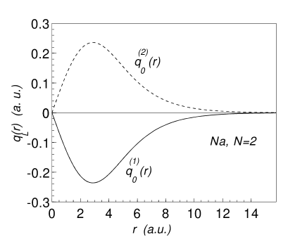
Figure 1: Source terms $q_{l=0,\sigma}^{(1)}$ and $q_{l=0,\sigma}^{(2)}$ in atomic units for Na₂. As is obvious, the two terms are equal and opposite in sign, so that the orbital shift for $N=2$ vanishes and the KLI and OEP results coincide.

In Fig.1, the source term components $q_{l=0,\sigma}^{(1)}$ and $q_{l=0,\sigma}^{(2)}$ are plotted as functions of radial coordinate. As is seen, they are equal and opposite in sign so that they lead to zero orbital shift, i.e., $\xi_{l=0,\sigma}(r)=0$. This result in turn leads to the coincidence of the KLI and OEP results.

In Figs. 2(a) and 2(b) the self-consistent source terms $q_{l\sigma}(r)$ of Eq.(22) are plotted as functions of radial coordinate for Na₈ and Li₁₈, respectively. The corresponding orbital shifts $\xi_{l\sigma}$ are shown in Figs. 3(a) and 3(b). It should be noted that $q_{i\sigma}(r)$ and $\xi_{i\sigma}(r)$ must behave such that

$$\int d{{\bf r}}\;Q_{i\sigma}({{\bf r}})\phi_{i\sigma}({{\bf r}})=0$$ (27)

and

$$\int d{{\bf r}}\;\psi^{*}_{i\sigma}({{\bf r}})\phi_{i\sigma}({{\bf r}})=0$$ (28)

are satisfied.

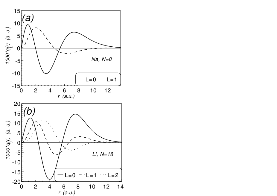
Figure 2: (a)-Source terms $q_{l\sigma}$ in atomic units for Na₈, and (b)- for Li₁₈. For Na₈, only $l=0$ and $l=1$ orbitals are occupied for each spin component whereas, for Li₁₈, the orbitals with $l=0,1,2$ are occupied.

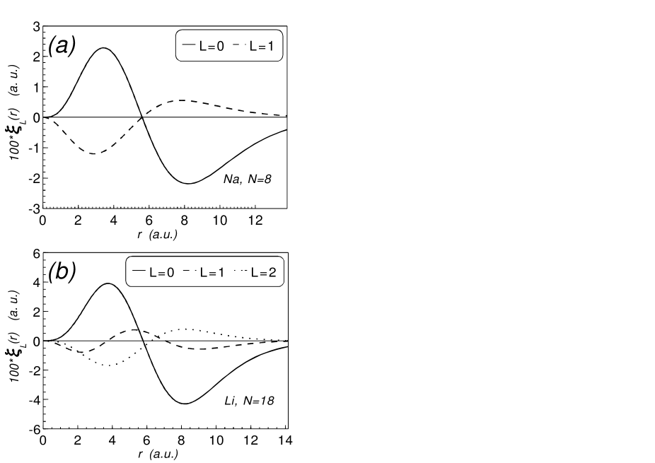
Figure 3: Orbital shifts $\xi_{l\sigma}$ in atomic units (a)- for Na₈ and (b)- for Li₁₈.

In order to solve the self-consistent OEP equations, we use the KLI self-consistent results as input. For the KLI calculations, we use [Eq.(23) of Ref.KummelPRB03 with $\psi_{i\sigma}({{\bf r}})=0$]:

$$v_{x\sigma}^{\rm KLI}({{\bf r}})=\frac{1}{2n_{\sigma}({{\bf r}})}\sum_{i=1}^{N_{\sigma}}\left\{\phi_{i\sigma}({{\bf r}})\phi_{i\sigma}^{*}({{\bf r}})u_{xi\sigma}({{\bf r}})\right.$$

$$\left.+|\phi_{i\sigma}({{\bf r}})|^{2}(\bar{v}_{xi\sigma}-\bar{u}_{xi\sigma})\right\}+c.c.$$ (29)

The self-consistent exchange potentials of Li₂ and Al₁₈ are plotted in Figs. 4(a) and 4(b), respectively. For comparison, the LSDA exchange-correlation potentials are also included. One notes that in Li₂ case, the KLI and OEP potentials are completely coincident whereas, in Al case, the KLI and OEP coincide only in the asymptotic region. On the other hand, the LSDA potential, because of wrong exponential asymptotic behavior, decays faster than the KLI or OEP, which have correct asymptotic behaviors of $1/r$. In the Al case, $N=18$ refers to the number of electrons which corresponds to the number $n=6$ of Al atoms.

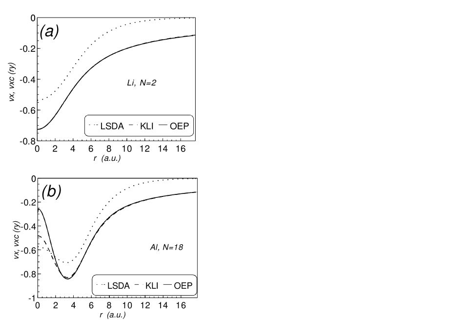
Figure 4: Exchange potentials in KLI and OEP and exchange-correlation potentials in LSDA, in Rydbergs, for (a)- Li₂ and, (b)- for Al₁₈. Here 18 refers to the electrons which is equivalent to 6 Al atoms. In Li₂ the KLI and OEP completely coincide whereas, in Al₁₈ the coincidence occurs at asymptotic region. The LSDA has wrong exponential decay whereas, KLI and OEP have correct $1/r$ decays.

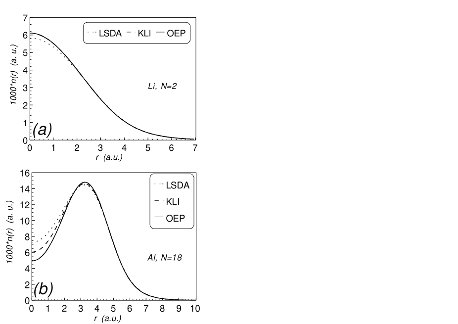
Figure 5: Densities in atomic units for Li₂ and, (b)- for Al₁₈. Here, as in potentials, we have full coincidence for Li₂ and asymptotic coincidence for Al₁₈.

In Figs. 5(a) and 5(b), we have shown the self-consistent densities for Li₂ and Al₁₈, respectively. As in the potential case, for Li₂ the KLI and OEP densities completely coincide whereas, in Al₁₈ the coincidence is only at the asymptotic region.

In Table 1 we have listed the self-consistent calculated ground state properties of the closed-shell clusters of Al, Li, Na, K, Cs for $N=$2, 8, 18, 20, 34, and 40. For comparison of our OEP results with those obtained by Engel and Vosko (EV)EV , we have also included those results for Al, Na, and Cs. The EV results are based on gradient expansion which, in principle, is valid only for slow variations of density as in a bulk solid. However, for finite systems such as clusters or surfaces, the EV results may differ from the exact OEP results. Comparison of our OEP total energies with those of EV for Na clusters shows a difference of $0.002\%$ on average. On the other hand, the EV exchange energies differ, on average, by $0.001\%$ and the average difference in $\varepsilon_{H}$ is $0.08\%$. From the computational costs point of view, these quite small differences makes the EV method advantageous for calculations within above mentioned accuracies.

Now we compare the total energies and the exchange energies in the KLI, OEP, and LSDA schemes. Comparison of the total energies shows that the OEP energies, on the average, are $1.2\%$ less than those of the KLI. We do not compare the total energies of OEP and LSD because in LSD there exist a correlation contribution. On the other hand, comparison of the exchange energies shows that on the average, the exchange energies in the OEP is $0.33\%$ more negative than that of the KLI whereas, it is $9\%$ more negative than the LSD.

An other feature in OEP which should be noted is the contraction of the KS eigenvalue bands relative to those of KLI. The results in Table 1 show that for all $N$, the relation $\Delta^{\rm OEP}<\Delta^{KLI}$ holds. Here, $\Delta=\varepsilon_{H}-\varepsilon_{L}$ is the difference between the maximum occupied and minimum occupied KS eigenvalues. For $N$=2, we have $\Delta=0$. The results show that the maximum relative contraction,$|\Delta^{\rm OEP}-\Delta^{KLI}|/\Delta^{KLI}$, is 2.6$\%$ which corresponds to Cs₁₈.

Table 1: Absolute values of total and exchange energies as well as highest occupied and lowest occupied Kohn-Sham eigenvalues in Rydbergs. The LSDA total energies include the correlation energies as well.

			LSDA				KLI				OEP				EV
Atom	$r_{s}$	$N$	$-E$	$-E_{x}$	$-\varepsilon_{L}$	$-\varepsilon_{H}$	$-E$	$-E_{x}$	$-\varepsilon_{L}$	$-\varepsilon_{H}$	$-E$	$-E_{x}$	$-\varepsilon_{L}$	$-\varepsilon_{H}$	$-E$	$-E_{x}$	$-\varepsilon_{H}$
Al	2.07	2	0.0944	0.5936	0.3821	0.3821	0.0557	0.7016	0.5973	0.5973	0.0557	0.7016	0.5973	0.5973	0.0557	0.7016	0.5973
		8	0.3087	2.7822	0.6957	0.3806	-0.0660	3.0178	0.8552	0.5418	-0.0653	3.0248	0.8507	0.5416	-0.0653	3.0248	0.5417
		18	0.4519	6.6899	0.8606	0.3411	-0.6023	7.0693	0.9710	0.4618	-0.5998	7.0987	0.9608	0.4600	-0.5998	7.0987	0.4600
		20	0.6444	7.4183	0.8556	0.3215	-0.5493	7.7898	0.9662	0.4333	-0.5480	7.8071	0.9618	0.4326	-0.5480	7.8071	0.4316
		34	0.7603	13.1379	0.9522	0.3103	-1.4409	13.7043	1.0356	0.4066	-1.4354	13.7536	1.0298	0.4027	-1.4354	13.7535	0.4027
		40	1.0806	15.3585	0.9497	0.3082	-1.6022	15.8635	1.0369	0.3996	-1.6000	15.8913	1.0307	0.3956	-1.6001	15.8913	0.3955
Li	3.28	2	0.2327	0.4324	0.2736	0.2736	0.1866	0.5074	0.4203	0.4203	0.1866	0.5074	0.4203	0.4203	-	-	-
		8	1.0141	1.9015	0.4074	0.2752	0.6708	2.0538	0.5097	0.3779	0.6714	2.0591	0.5076	0.3781	-	-	-
		18	2.3050	4.4733	0.4714	0.2598	1.3930	4.7233	0.5404	0.3338	1.3952	4.7474	0.5352	0.3328	-	-	-
		20	2.6056	4.9417	0.4681	0.2303	1.5677	5.1710	0.5316	0.2992	1.5689	5.1842	0.5295	0.3000	-	-	-
		34	4.4619	8.6619	0.5065	0.2494	2.5990	9.0347	0.5570	0.3061	2.6040	9.0778	0.5533	0.3037	-	-	-
		40	5.2635	10.1016	0.5014	0.2267	2.9843	10.3981	0.5491	0.2794	2.9865	10.4195	0.5464	0.2783	-	-	-
Na	3.93	2	0.2462	0.3787	0.2381	0.2381	0.1988	0.4428	0.3627	0.3627	0.1988	0.4428	0.3627	0.3627	0.1988	0.4428	0.3626
		8	1.0737	1.6290	0.3333	0.2402	0.7465	1.7551	0.4177	0.3249	0.7470	1.7598	0.4162	0.3251	0.7470	1.7598	0.3252
		18	2.4664	3.8049	0.3777	0.2297	1.6128	4.0135	0.4338	0.2896	1.6148	4.0354	0.4298	0.2888	1.6148	4.0354	0.2888
		20	2.7664	4.1991	0.3748	0.2018	1.7944	4.3852	0.4250	0.2577	1.7956	4.3974	0.4237	0.2588	1.7956	4.3974	0.2600
		34	4.7746	7.3347	0.4022	0.2232	3.0446	7.6461	0.4424	0.2679	3.0493	7.6870	0.4392	0.2659	3.0494	7.6870	0.2662
		40	5.6075	8.5495	0.3976	0.2002	3.4899	8.7840	0.4337	0.2412	3.4920	8.8038	0.4320	0.2410	3.4920	8.8036	0.2414
K	4.96	2	0.2448	0.3174	0.1981	0.1981	0.1970	0.3693	0.2979	0.2979	0.1970	0.3693	0.2979	0.2979	-	-	-
		8	1.0596	1.3306	0.2594	0.2006	0.7553	1.4280	0.3245	0.2658	0.7557	1.4319	0.3235	0.2660	-	-	-
		18	2.4442	3.0822	0.2874	0.1943	1.6667	3.2447	0.3294	0.2389	1.6685	3.2639	0.3266	0.2383	-	-	-
		20	2.7275	3.3986	0.2851	0.1700	1.8420	3.5380	0.3214	0.2120	1.8431	3.5490	0.3211	0.2134	-	-	-
		34	4.7230	5.9117	0.3030	0.1908	3.1617	6.1552	0.3320	0.2229	3.1662	6.1934	0.3295	0.2214	-	-	-
		40	5.5338	6.8879	0.2995	0.1701	3.6226	7.0565	0.3234	0.1988	3.6247	7.0744	0.3230	0.1994	-	-	-
Cs	5.63	2	0.2382	0.2875	0.1789	0.1789	0.1907	0.3335	0.2669	0.2669	0.1907	0.3335	0.2669	0.2669	0.1907	0.3335	0.2669
		8	1.0252	1.1904	0.2271	0.1816	0.7341	1.2742	0.2833	0.2376	0.7345	1.2778	0.2826	0.2378	0.7345	1.2777	0.2378
		18	2.3652	2.7459	0.2490	0.1768	1.6290	2.8866	0.2846	0.2144	1.6307	2.9044	0.2823	0.2139	1.6307	2.9043	0.2132
		20	2.6351	3.0268	0.2471	0.1548	1.7969	3.1446	0.2772	0.1904	1.7980	3.1553	0.2773	0.1920	1.7980	3.1553	0.1925
		34	4.5646	5.2538	0.2613	0.1743	3.0932	5.4652	0.2851	0.2007	3.0974	5.5020	0.2830	0.1994	3.0974	5.5020	0.1974
		40	5.3452	6.1206	0.2584	0.1554	3.5445	6.2591	0.2770	0.1787	3.5462	6.2788	0.2766	0.1791	3.5465	6.2763	0.1795

IV Summary and Conclusion

In this work, we have considered the exchange-only jellium model in which we have used the exact orbital-dependent exchange functional. This model is applied for the closed-shell simple metal clusters of Al, Li, Na, K, and Cs. For the local exchange potential in the KS equation, we have solved the OEP integral equation by the iterative method proposed recently by Kümmel and Perdew KummelPRB03 . By solving the self-consistent KS equations, we have obtained the ground state energies of the closed-shell clusters ($N=2,8,18,20,34,40$) for the three schemes of LSD, KLI, and OEP. The KLI and OEP results are the same for neutral two-electron clusters. However, for $N\neq 2$, the densities and potentials in the KLI and OEP coincide for large $r$ values. The OEP exchange and effective potentials shows correct behavior of $1/r$ compared to the incorrect exponential behavior in the LSD. The total energies in the OEP are more negative than the KLI by $1.2\%$ on the average. On the other hand, the exchange energies in the OEP is about $0.33\%$ more negative than that in the KLI whereas, it is about $9\%$ more negative than that in the LSDA. The widths of the occupied bands, $\varepsilon_{H}-\varepsilon_{L}$ in the OEP are contracted relative to those in the KLI by at most $2.6\%$ which corresponds to Cs₁₈. In spite of the validity of the gradient expansion method for slow variations in density, comparison of our OEP results with those of EV shows an excellent agreement.

- (1) W. Kohn and L. J. Sham, Phys. Rev. 140, A1133 (1965).
- (2) J. P. Perdew, Phys. Rev. Lett. 55, 1665 (1985).
- (3) J. P. Perdew, K. Burke, and M. Ernzerhof, Phys. Rev. Lett. 77, 3865 (1996).
- (4) P. Hohenberg and W. Kohn, Phys. Rev. 136, B864 (1964).
- (5) K. Burke, M. Ernzerhof, and J. P. Perdew, J. Chem. Phys. 110, 2029 (1999).
- (6) R. T. Sharp, and G. K. Horton, Phys. Rev. 90, 317 (1953).
- (7) J. D. Talman and W. F. Shadwick, Phys. Rev. A 14, 36 (1976).
- (8) V. Sahni, J. Gruenebaum, and J. P. Perdew, Phys. Rev. B 26, 4371 (1982).
- (9) M. Städele, M. Moukara, J. A. Majewski, P. Vogl, and A. Görling, Phys. Rev. B 59, 10031 (1999).
- (10) A. Görling, Phys. Rev. Lett. 83, 5459 (1999).
- (11) S. Ivanov, S. Hirata, and R. J. Bartlett, Phys. Rev. Lett. 83, 5455 (1999).
- (12) S. Kümmel and J. P. Perdew, Phys. Rev. Lett. 90, 043004 (2003).
- (13) S. Kümmel and J. P. Perdew, Phys. Rev. B 68, 035103 (2003).
- (14) M. Payami, J. Chem. Phys. 111, 8344 (1999).
- (15) M. Payami, J. Phys.: Condens. Matter 13, 4129 (2001).
- (16) M. Payami, Can. J. Phys. 82, 239 (2004).
- (17) J. B. Krrieger, Y. Li, and G. J. Iafrate, Phys. Rev. A 46, 5453 (1992).
- (18) E. Engel and S. H. Vosko, Phys. Rev. B 50, 10498 (1994). The unpublished Al and Cs data have been provided by E. Engel.