Gene regulatory networks: a coarse-grained, equation-free approach to multiscale computation

Abstract: We present computer-assisted methods for analyzing stochastic models of gene regulatory networks. The main idea that underlies this equation-free analysis is the design and execution of appropriately-initialized short bursts of stochastic simulations; the results of these are processed to estimate coarse-grained quantities of interest, such as mesoscopic transport coefficients. In particular, using a simple model of a genetic toggle switch, we illustrate the computation of an effective free energy $\Phi$ and of a state-dependent effective diffusion coefficient $D$ that characterize an unavailable effective Fokker-Planck equation. Additionally we illustrate the linking of equation-free techniques with continuation methods for performing a form of stochastic “bifurcation analysis”; estimation of mean switching times in the case of a bistable switch is also implemented in this equation-free context. The accuracy of our methods is tested by direct comparison with long-time stochastic simulations. This type of equation-free analysis appears to be a promising approach to computing features of the long-time, coarse-grained behavior of certain classes of complex stochastic models of gene regulatory networks, circumventing the need for long Monte Carlo simulations.

1 Introduction

Various ways to model gene-regulatory networks exist, ranging from logical (boolean), to stochastic (Monte Carlo methods) or deterministic (ordinary differential equations) models (for recent reviews see [35, 19, 21]). Each modeling approach has its advantages and disadvantages. One advantage of stochastic modeling is that it takes into account fluctuations due to the inherently random nature of biochemical reactions. This intrinsic noise gives rise to significant effects when either the molecular abundances of protein or mRNA molecules are small or the kinetics of the transitions between the chemical states of the promoter are slow [23, 21].

The established approach for stochastic modeling of spatially homogeneous chemical systems was introduced by Gillespie [13]. The Gillespie Stochastic Simulation Algorithm (SSA) is based on repeatedly answering two questions: when does the next chemical reaction occur and what kind of reaction is it? Gillespie [13] derived a simple way to answer these two questions that reduces the problem to a continuous-time discrete space Markov process.

The SSA generates exact sample paths of the stochastic process and, for sufficiently large networks, it is computationally more efficient than solving the chemical master equation. However, the large size of naturally occurring gene regulatory networks makes even the SSA computationally intensive and practically impossible to use for computing the long-time behavior of the network. Consequently, an important restriction of stochastic computations for many networks of interest is that we can efficiently run stochastic Gillespie-based simulators for short times only. It is therefore natural to look for computational methods that use only short time simulations (and as few of these as necessary) to compute the required information for the system. Such a computer-assisted approach is presented in this paper.

Model reduction often provides a natural path to efficient simulation of a complicated model. As in other branches of physical modeling, separation of time scales can lead to successful model reduction in gene regulatory network modeling. Separation of time scales is frequently present in this context because synthesis and degradation of new proteins and transcripts usually occurs on a slower time scale than processes that change the chemical state of proteins (e.g., multimerization, protein/DNA interactions, phosphorylation). Theoretical methods for stochastic model reduction that take advantage of separation of time scales are being developed (e.g. [23, 5, 17, 31]). Analytical reduction techniques assume that fast variables are in quasi-steady state with respect to the remaining slow variables. If the quasi-steady state distributions conditioned on the slow variables can be determined, then they can be used to eliminate the fast variables.

Our approach is also based on (and takes advantage of) the separation of time scales and the approximation (computationally, on the fly) of quasi-steady marginal distributions (conditioned on the slow variables). The main feature of our approach, as will become apparent through its description and illustration, is that we do not “first reduce and then simulate the reduced model”; our methods come in the form of wrappers around a black box dynamic simulator, and could equally well be applied to the most detailed stochastic version of the network model or to its best explicit reduction already available. In our approach, results about the long-term dynamic behavior of a stochastic simulator do not come from long-term simulation; they come from the design, execution and processing of the results of “intelligently designed” short bursts of direct dynamic simulation.

We believe it is useful to draw here an analogy with the study of nonlinear dynamics in systems of ODEs. Long-term information in the form of detailed bifurcation diagrams can be obtained from long dynamic integration; yet the same information is much more systematically and economically obtained through different algorithms using the same model: bifurcation, stability and continuation methods. It is this alternative to direct, long-term stochastic simulation (whether with the full detailed network model or with any good analytical reduction of it) that our approach makes available to the modeler. Ours is a “design of computational experiments” approach; it is guided by model reduction, but a reduced model is never explicitly obtained.

The remainder of the paper is organized as follows. In Section 2, we introduce the genetic toggle switch as a simple model to illustrate our methods, and we specify the main questions that one would like to answer with these techniques. In Section 3, we present the general mathematical framework and main ideas of equation-free analysis [24, 8, 12, 36, 16]. In Section 4, we present an analysis of a deterministic model of the genetic toggle switch to provide insight into this system. We also introduce several stochastic models of increasing complexity that are used to illustrate equation-free analysis. In Section 5, we compute the effective free energies and the associated stationary distributions for the stochastic models described in Section 4. Equation-free bifurcation analysis is then presented, and, in bistable cases, the mean first passage times for the system to switch between apparent stable fixed points are computed. We end with a discussion of the equation-free approach, its strengths, weaknesses, relations to other current methods for the acceleration of SSA-type simulations (e.g. [23, 5, 17, 31, 1]) and its possible extensions in Section 6. In particular, we will discuss the applicability of our methods to more complicated gene-regulatory networks.

2 Model Description

Our illustrative example is a two gene network in which each protein represses the transcription of the other gene (mutual repression). This type of system has been engineered in E. coli and is often referred to as a genetic toggle switch [9, 18]. The advantage of this simple system is that it allows us to test the accuracy of equation-free methods by direct comparisons with results from long-time stochastic simulations. In Section 6, we discuss the applicability of our methods to more complex problems where long direct stochastic simulation is impossible and the accuracy must be checked by on line a posteriori error estimates.

A simple version of the genetic toggle switch is schematically drawn in Figure 1.

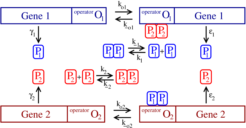
Figure 1: A schematic diagram of the genetic toggle switch.

The system contains two proteins $P_{1}$ and $P_{2}$. The production of $P_{1}$ ($P_{2}$) depends on the chemical state of the upstream operator $O_{1}$ ($O_{2}$). If $O_{1}$ is empty then $P_{1}$ is produced at the rate $\gamma_{1}$ and if $O_{1}$ is occupied by a dimer of $P_{2}$, then protein $P_{1}$ is produced at a rate $\epsilon_{1}<\gamma_{1}.$ Similarly, if $O_{2}$ is empty then $P_{2}$ is produced at the rate $\gamma_{2}$ and if $O_{2}$ is occupied by a dimer of $P_{1}$, then protein $P_{2}$ is produced at a rate $\epsilon_{2}<\gamma_{2}.$ Note that for simplicity, transcription and translation are described by a single rate constant. The biochemical reactions and rate constants that correspond to the processes shown in Figure 1 are

$${\mbox{ \raise 2.42131pt\hbox{$\emptyset$}}}\quad\;\mathop{\stackrel{{\scriptstyle\displaystyle\longrightarrow}}{{\longleftarrow}}}^{\gamma_{1}O_{1}+\varepsilon_{1}\overline{P_{2}P_{2}O_{1}}}_{\delta_{1}}\quad{\mbox{ \raise 2.42131pt\hbox{$P_{1}$}}}$$ (2.1)

$${\mbox{ \raise 2.42131pt\hbox{$\emptyset$}}}\quad\;\mathop{\stackrel{{\scriptstyle\displaystyle\longrightarrow}}{{\longleftarrow}}}^{\gamma_{2}O_{2}+\varepsilon_{2}\overline{P_{1}P_{1}O_{2}}}_{\delta_{2}}\quad{\mbox{ \raise 2.42131pt\hbox{$P_{2}$}}}$$ (2.2)

$${\mbox{ \raise 2.42131pt\hbox{$P_{1}+P_{1}$}}}\quad\;\mathop{\stackrel{{\scriptstyle\displaystyle\longrightarrow}}{{\longleftarrow}}}^{k_{1}}_{k_{-1}}\quad{\mbox{ \raise 2.42131pt\hbox{$\overline{P_{1}P_{1}}$}}}$$ (2.3)

$${\mbox{ \raise 2.42131pt\hbox{$P_{2}+P_{2}$}}}\quad\;\mathop{\stackrel{{\scriptstyle\displaystyle\longrightarrow}}{{\longleftarrow}}}^{k_{2}}_{k_{-2}}\quad{\mbox{ \raise 2.42131pt\hbox{$\overline{P_{2}P_{2}}$}}}$$ (2.4)

$${\mbox{ \raise 2.42131pt\hbox{$\overline{P_{2}P_{2}}+O_{1}$}}}\quad\;\mathop{\stackrel{{\scriptstyle\displaystyle\longrightarrow}}{{\longleftarrow}}}^{k_{o1}}_{k_{-o1}}\quad{\mbox{ \raise 2.42131pt\hbox{$\overline{P_{2}P_{2}O_{1}}$}}}$$ (2.5)

$${\mbox{ \raise 2.42131pt\hbox{$\overline{P_{1}P_{1}}+O_{2}$}}}\quad\;\mathop{\stackrel{{\scriptstyle\displaystyle\longrightarrow}}{{\longleftarrow}}}^{k_{o2}}_{k_{-o2}}\quad{\mbox{ \raise 2.42131pt\hbox{$\overline{P_{1}P_{1}O_{2}}$}}}$$ (2.6)

where the overbars denote complexes. Equation (2.1) describes production and degradation of protein $P_{1}$, equation (2.2) describes production and degradation of protein $P_{2}$, equations (2.3) and (2.4) are dimerization reactions and equations (2.5) and (2.6) represent the binding and dissociation of the dimer and DNA.

Single cell fluorescence measurements can be used to measure intercellular variability in protein expression levels. Therefore it is important to have efficient methods for computing the steady-state distribution of protein abundances from stochastic models similar to the one defined by (2.1) – (2.6). For moderately complex systems using long-time Monte Carlo simulations quickly becomes computationally prohibitive. We will illustrate how equation-free analysis can overcome this difficulty by accelerating the exploration of certain features of the long-term dynamics of the stochastic simulation. For certain values of the model parameters, the genetic toggle switch is bistable. If the system is described in terms of ordinary differential equations (ODEs) for the protein concentrations, then standard bifurcation analysis (numerical continuation methods) can be applied to determine the regions of parameter space in which bistability occurs. Using the model described by (2.1) – (2.6) as an example, we show how to extend these techniques to stochastic models. An important quantity that characterizes the dynamics of bistable stochastic systems is the average time for spontaneous transitions between stable steady states to occur. We will illustrate how this mean first passage time can be computed by using only short-time simulations.

3 Equation-Free Analysis: Mathematical Framework

Let us suppose that we have a well-stirred mixture of chemically reacting species; our main assumption is that the evolution of the system can be described in terms of a single, slowly evolving random variable $Q$ (the approach carries through for the case of a small number of slow variables, but in this paper we will focus on the single slow variable case). $Q$ might be the concentration of one of the chemical species or some function of the concentrations. Let $\bf R$ denote a vector of the other (fast, “slaved” system variables). Our assumption implies that the evolution of the system can be approximately described by the time-dependent probability density function $f(q,t)$ for the slow variable $Q$ that evolves according to following effective Fokker-Planck equation [33]:

$$\frac{\partial f}{\partial t}=\frac{\partial}{\partial q}\left(\frac{\partial}{\partial q}[D(q)f(q,t)]-V(q)f(q,t)\right).$$ (3.1)

If the effective drift $V(q)$ and diffusion coefficient $D(q)$ could be explicitly written down as function of $q$, then (3.1) can be used to compute interesting properties of the system (e. g., the steady state distribution). Note that in addition to the assumption of a single slow variable, the validity of equation (3.1) requires sufficiently large molecular abundances and sufficiently fast chemical kinetics for transitions in the chemical state of the operator [9, 23]. Assuming that (3.1) provides a good approximation, we make use of the following formulas for the drift and diffusion coefficient [16, 20, 25, 37]

$$V(q) = \lim_{\Delta t\to 0}\frac{<Q(t+\Delta t)-q\,|\,Q(t)=q>}{\Delta t}$$ (3.2)

$$D(q) = \frac{1}{2}\,\lim_{\Delta t\to 0}\frac{<[Q(t+\Delta t)-q]^{2}\,|\,Q(t)=q>}{\Delta t}.$$ (3.3)

As described below, estimates of these two quantities can be found by using short-time bursts of appropriately initialized stochastic simulations. The steady solution of (3.1) is proportional to $\exp[-\beta\Phi(q)]$, where the effective free energy $\Phi(q)$ is defined as

$$\frac{\Phi(q)}{k_{B}T}\equiv\beta\Phi(q)=-\int_{0}^{q}\frac{V(q^{\prime})}{D(q^{\prime})}\mbox{d}q^{\prime}+\ln D(q)+\mbox{constant}.$$ (3.4)

Consequently, computing the effective free energy and the steady state probability distribution also can be accomplished without the need for long-time stochastic simulations.

A procedure for computationally estimating $V(q)$ and $D(q)$ is as follows:

(A) Given $Q=q$, approximate the conditional density $P({\bf r}|Q=q)$ for the fast variables $\bf R$. Details of this preparatory step are given below.

(B) Use $P({\bf r}|Q=q)$ from the step (A) to determine appropriate initial conditions for the short simulations and run multiple realizations for time $\Delta t$. Use the results of these simulations and the definitions (3.2) and (3.3) to estimate the average velocity $V(q)$ and effective diffusion coefficient $D(q)$.

(C) Repeat steps (A) and (B) for sufficiently many values of $Q$ and then compute $\Phi(q)$ using formula (3.4) and numerical quadrature.

A very important feature of this algorithm is that it is trivially parallelizable (different realizations of short simulations starting at “the same $q$” as well a simulation realizations starting at different $q$ values can be run independently, on multiple processors).

In order to use the algorithm (A) – (C), we have to specify how the step (A) is performed. There are several computational options to approximate the conditional density $P({\bf r}|Q=q).$ The simplest approximation is to estimate (through numerical experiments) the conditional mean $<\!\!{\bf R}|{Q=q}\!\!>$ and approximate $P({\bf r}|Q=q)$ as a Dirac delta function $\delta({\bf r}-<\!\!{\bf R}|Q=q\!\!>)$. Then the step (A) reads as follows:

(A1) Given $Q=q$, pick an initial guess for the conditional mean of ${\bf R}$. Denote the initial guess as $<\!\!{\bf R}(0)\!\!>$. Run multiple realizations for a short time $\delta t$ and compute $<\!\!{\bf R}(\delta t)\!\!>.$ This procedure defines the mapping $<\!\!{\bf R}(0)\!\!>\to<\!\!{\bf R}(\delta t)\!\!>.$ Find the steady state of this mapping using standard numerical methods. The steady state is the required conditional average $<\!\!{\bf R}|{Q=q}\!\!>.$ Initialize ${\bf R}(0)$ as $<\!\!{\bf R}|{Q=q}\!\!>$ in all realizations in part (B) of the algorithm.

Another option is to approximate $P({\bf r}|Q=q)$ as a distribution characterized by a few parameters, e.g. as a Gaussian distribution with mean $\boldsymbol{\mu}$ and variance $\boldsymbol{\sigma}.$ This can be done as follows:

(A2) Given $Q=q$, pick initial guesses for the mean $\boldsymbol{\mu}(0)$ and variance $\boldsymbol{\sigma}(0)$ of the conditional distribution function $P({\bf r}|Q=q)$. Use this distribution to generate many realizations of ${\bf R}(0)$. Using these realizations as initial conditions, run stochastic simulations for a short time $\delta t$ and compute ${\bf R}(\delta t).$ Computing mean and variance of ${\bf R}(\delta t),$ we obtain the mapping $[\boldsymbol{\mu}(0),\boldsymbol{\sigma}(0)]\to[\boldsymbol{\mu}(\delta t),\boldsymbol{\sigma}(\delta t)].$ Next use standard numerical methods to find the steady state $[\boldsymbol{\mu},\boldsymbol{\sigma}]$ of this mapping and approximate $P({\bf r}|Q=q)$ as a Gaussian distribution with mean $\boldsymbol{\mu}$ and variance $\boldsymbol{\sigma}.$

The conditional density $P({\bf r}|Q=q)$ can be also approximated by other basis functions. It is straightforward to generalize (A1) or (A2) to such a case. The better the approximation of $P({\bf r}|Q=q)$ we have, the shorter the time step, $\delta t$, required in the step (B) to achieve the same accuracy. So, a better approximation of $P({\bf r}|Q=q)$ in step (A) decreases the computational intensity of step (B). On the other hand, step (A) is more computationally intensive if we want to obtain a better approximation of $P({\bf r}|Q=q)$. One possibility for generating a better approximation of $P({\bf r}|Q=q)$ is to use a “run-and-reset” procedure as was done in [8]. This is accomplished as follows.

(A3) Given $Q=q$, initialize the other variables ${\bf R}\equiv{\bf R}(0)$ of the system. Run stochastic simulations for the short time $\delta t$. Then reset the value of $Q(\delta t)$ to its original value $q$ keeping ${\bf R}$ unchanged. Repeat this procedure for many time steps and compute the conditional density $P({\bf r}|Q=q)$ as a histogram of the recorded values of ${\bf R}$.

The approach (A3) attempts to compute the $P({\bf r}|Q=q)$ effectively by successive substitution, without resorting to numerical algorithms of the Newton-Raphson type for locating fixed points of mappings; we will return to this latter issue in the Discussion section. In our illustrative computations in Section 5, we use step (A) in the form (A1) or (A3) for the simple stochastic models described below. Both give good results for our illustrative example. Since (A1) works for sufficiently long times $\delta t$, there is no need to use (A2) or higher order approximations. For some stochastic simulations of our model problem, we also use slightly modified versions of the methods (A1) or (A3) as will be described in Section 5.

3.1 Bifurcations

In deterministic problems, we often summarize the parametric dependence of the long-term dynamics in terms of bifurcation diagrams; for example, we may plot the steady states of a deterministic set of ODEs as a function of a distinguished bifurcation parameter. Several excellent continuation methods have been developed, implemented and made available for this purpose over the years, such as AUTO [6, 7].

Here we illustrate how these methods can be extended to stochastic models [24, 12, 37, 26, 27]. We assume, as above, that we have a stochastic problem that can be effectively described by a single variable $Q.$ Let $\gamma$ be the bifurcation parameter. The first two steps in the algorithm are as follows:

($\mathbb{A}$) Given $Q=q$ and the value of the bifurcation parameter $\gamma$, compute the conditional density $P({\bf r}|Q=q)$ using step (A) of the previous algorithm.

($\mathbb{B}$) Using $P({\bf r}|Q=q)$ from step ($\mathbb{A}$) to determine the initial conditions, run multiple stochastic simulations for a short time $\Delta t$ and compute the conditional average $<\!\!Q(\Delta t)|Q(0)=q\!\!>$.

Steps $\mathbb{A}$ and $\mathbb{B}$ define the mapping $(Q(0),\gamma)\to<\!\!Q(\Delta t)\!\!>$. We denote this mapping as $F$, i.e. $F(Q,\gamma)=<\!\!Q(\Delta t)\!\!>.$ Our goal is to track the fixed points of $F$ (i.e. $F(Q,\gamma)=Q$) as the bifurcation parameter $\gamma$ is varied. To do this, we first use a Newton-Raphson algorithm to find two steady states $(Q_{1},\gamma_{1})$ and $(Q_{2},\gamma_{2})$ which are sufficiently close to each other (note that one can estimate the derivative of $F(Q,\gamma)$ numerically by evaluating $F(Q,\gamma)$ at different points). Then, in a parameter continuation context, we choose a small parameter $\delta$ (which can be modified adaptively during the computation) and find the next steady state using continuation. That is, the next values of $Q$ and $\gamma$ are found by solving the following system of equations

$$\left\{\begin{array}[]{ccc}Q-F(Q,\gamma)&=&0,\\ (Q-Q_{2})(Q_{2}-Q_{1})+(\gamma-\gamma_{2})(\gamma_{2}-\gamma_{1})-\delta&=&0.\end{array}\right.$$ (3.5)

To find the solution of (3.5), we estimate the Jacobian numerically by evaluating $F(Q,\gamma)$ at several points and then use Newton-Raphson algorithm. When the number of variables starts becoming large, matrix-free methods of iterative numerical linear algebra (such as Broyden, or Newton-Krylov GMRES [22]) can be used to solve for the fixed point, as opposed to full numerical Jacobian estimation. The fixed points computed this way provide, under certain conditions, good estimates of the critical points (minima, saddles) of the effective potential $\Phi(q)$) as a function of a model parameter $\gamma$; this issue is discussed extensively in [26, 27, 3, 37], and we will return to it again in the Discussion section.

3.2 First Passage Time

Suppose that we have a bistable stochastic system. That is, the effective free energy $\Phi(q)$ has two local minima [14] - see Figure 2. Then an important quantity characterizing the long-time system dynamics is the mean time for spontaneous transitions to occur between the stable steady states. Let $q_{m}<q_{M}$ denote the two stable steady states and let $q_{u}$ be the unstable state (i.e. local maximum of $\Phi(q)$).

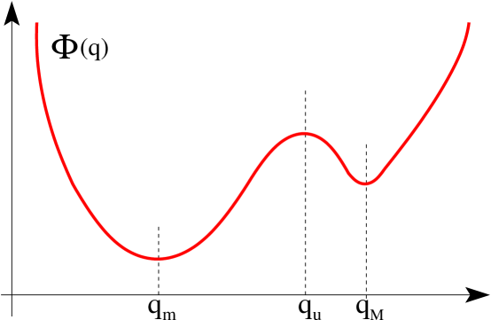
Figure 2: Potential $\Phi(q)$ of the bistable system.

Then we define the first passage time for transitions from $q_{m}$ to $q_{M}$ as $2\tau_{e}$ where $\tau_{e}$ is the average time for the system to reach the unstable steady state $q_{u}$ for the first time given that it starts at $q_{m}$. The factor of two occurs because once the system reaches the unstable steady state, half the time it returns the original stable steady state $q_{m}$ and the other half of the time it transitions to $q_{M}$.

Algorithm (A) – (C) gives a procedure to estimate the effective potential $\Phi(q)$ by running short simulations only. Once we have the effective potential, we can compute $\tau_{e}$ as follows [14]

$$\tau_{e;p}=\int_{q_{m}}^{q_{u}}\exp\left[\frac{\Phi(q)}{k_{B}T}\right]\int_{-\infty}^{q}\frac{1}{D(\xi)}\exp\left[-\frac{\Phi(\xi)}{k_{B}T}\right]\mbox{d}\xi\mbox{d}q$$ (3.6)

Equation (3.6) can be further simplified if the height of the potential barrier $[\Phi(q_{u})-\Phi(q_{m})]$ is large compared to the noise strength. In this case, the limit $q$ in the second integral can be replaced by $q_{s}$, allowing the two integrals to be evaluated separately

$$\tau_{e;p}\approx\int_{q_{m}}^{q_{u}}\exp\left[\frac{\Phi(q)}{k_{B}T}\right]\mbox{d}q\times\int_{-\infty}^{q_{u}}\frac{1}{D(q)}\exp\left[-\frac{\Phi(q)}{k_{B}T}\right]\mbox{d}q.$$

The main contribution of the first integral stems from the region around $q_{s}$, and the main contribution from the second integral stems from the region around $q_{m}$. Consequently, we expand $\Phi(q)$ according to

$$\Phi(q)\approx\Phi(q_{u})-\frac{1}{2}|\Phi^{\prime\prime}(q_{u})|(q-q_{u})^{2},\qquad\Phi(q)\approx\Phi(q_{m})+\frac{1}{2}\Phi^{\prime\prime}(q_{m})(q-q_{m})^{2}.$$

for the first and the second integral, respectively [33]. When these expansions are used in equation (3.2), the following result is obtained

$$\tau_{e;k}\approx\frac{4\pi k_{B}T}{[D(q_{u})+D(q_{m})]\sqrt{\Phi^{\prime\prime}(q_{m})|\Phi^{\prime\prime}(q_{u})|}}\exp\left[\frac{\Phi(q_{u})-\Phi(q_{m})}{k_{B}T}\right]$$ (3.7)

which is the generalization of Kramers’ formula to the case of a state dependent diffusion coefficient [33, 16]. Formulas (3.6) and (3.7) are both used in Section 5.2 to estimate $\tau_{e}.$

4 Analysis of the Model Problem

In this section, we study the behavior of the model given by equations (2.1) – (2.6). To provide insight into the problem, we start by analyzing the deterministic system. In Sections 4.2 and 4.3, we introduce two stochastic models that are simplified versions of the model defined by (2.1) – (2.6). We use these models because of the relative ease in performing long-time stochastic simulations with them; this allows the results from the equation-free analysis to be validated by direct comparisons with Monte Carlo simulations. We will also verify that the equation-free methods can be applied to the full model. As discussed below, for this case the long-time Monte Carlo simulations become computationally very expensive.

4.1 The Deterministic Model

To simplify the deterministic analysis, we make the assumption that equations (2.3) – (2.6) are at quasi-equilibrium and derive deterministic rate equations for the protein concentrations. Let $x_{1}$ and $x_{2}$ denote the average monomer concentrations of $P_{1}$ and $P_{2}$, respectively, and let $d_{1}$ and $d_{2}$ denote the respective dimer concentrations. Also, let $o_{1}$ and $o_{2}$ denote the probabilities that the operators $O_{1}$ and $O_{2}$ are not occupied. For the dimerization process the assumption of quasi-equilibrium implies

$$d_{1}=\frac{k_{1}}{k_{-1}}x_{1}^{2},\qquad\mbox{and}\qquad d_{2}=\frac{k_{2}}{k_{-2}}x_{2}^{2}.$$ (4.1)

Similarly, the quasi-equilibrium assumption for the operators implies that

$$o_{1}=\frac{k_{-o1}}{k_{-o1}+k_{o1}d_{2}},\qquad\mbox{and}\qquad o_{2}=\frac{k_{-o2}}{k_{-o2}+k_{o2}d_{1}}.$$ (4.2)

The total concentration of $P_{1}$ is given by $y_{1}=x_{1}+2d_{1}$. The total concentration $y_{1}$ evolves according to the following ordinary differential equation

$$\frac{\mbox{d}y_{1}}{\mbox{d}t}=\gamma_{1}o_{1}+\varepsilon_{1}(1-o_{1})-\delta_{1}x_{1}.$$ (4.3)

where $\delta$ is the degradation rate of the monomers, and it has been assumed that dimers are protected from degradation. Substituting $y_{1}=x_{1}+2d_{1}=x_{1}+2\frac{k_{1}}{k_{-1}}x_{1}^{2}$ into (4.3), we obtain

$$\left(1+4\frac{k_{1}}{k_{-1}}x_{1}\right)\frac{\mbox{d}x_{1}}{\mbox{d}t}=\gamma_{1}o_{1}+\varepsilon_{1}(1-o_{1})-\delta_{1}x_{1}$$

Finally, using (4.1) – (4.2) produces

$$\frac{\mbox{d}x_{1}}{\mbox{d}t}=\frac{1}{1+\kappa_{1}x_{1}}\left[\gamma_{1}\frac{1}{1+\omega_{1}x_{2}^{2}}+\varepsilon_{1}\frac{\omega_{1}x_{2}^{2}}{1+\omega_{1}x_{2}^{2}}-\delta_{1}x_{1}\right]$$ (4.4)

where the parameters $\kappa_{1}$ and $\omega_{1}$ are defined as follows

$$\kappa_{1}=4\frac{k_{1}}{k_{-1}},\qquad\mbox{and}\qquad\omega_{1}=\frac{k_{o1}}{k_{-o1}}\frac{k_{2}}{k_{-2}}.$$ (4.5)

Using similar reasoning an analogous equation for $x_{2}$ can be derived.

For simplicity, we will present the symmetric case in which the rate constants for processes involving $P_{1}$ are identical to those involving $P_{2}$. That is, we assume $\kappa\equiv\kappa_{1}=\kappa_{2},$ $\gamma\equiv\gamma_{1}=\gamma_{2},$ $\omega\equiv\omega_{1}=\omega_{2},$ and $\delta\equiv\delta_{1}=\delta_{2}$. Moreover, we assume that the production rate is zero if an operator is occupied, i.e. $\varepsilon_{1}=\varepsilon_{2}=0.$ Making these assumptions, (4.4) simplifies to

$$\frac{\mbox{d}x_{1}}{\mbox{d}t}=\frac{1}{1+\kappa x_{1}}\left[\frac{\gamma}{1+\omega x_{2}^{2}}-\delta x_{1}\right],$$ (4.6)

and the equation for $x_{2}$ is obtained by alternating the subscripts in the above equation. Hence, the problem has been reduced to a system of two equations with four parameters.

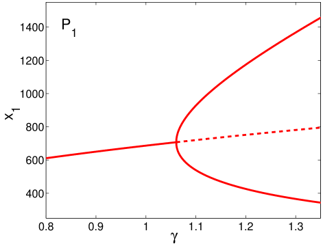
Figure 3: The dependence of the steady state values of $x_{1}$ on $\gamma$. The solid lines denote stable fixed points and the dashed line corresponds to unstable fixed points. In this figure and throughout the paper $\delta=0.00075$ and $\omega=2\times 10^{-6}.$

Note that the value of $\kappa$ does not influence the steady-state behavior of the system. In this paper, we fix the values of $\delta$ and $\omega$ to be $0.00075$ and $2\times 10^{-6}$, respectively.

The steady states values of $x_{1}$ as a function of $\gamma$ are shown in Figure 3. In this figure, solid lines denote stable steady states and dashed lines denote unstable steady states. For $\gamma<1.06$ there is a single steady state. At $\gamma=1.06$ a pitchfork bifurcation occurs, and for $\gamma>1.06,$ there exist three steady states. The steady state with $x_{1}=x_{2}$ is unstable and the other two steady states are stable.

Due to separation of time scales, the long-term dynamics of this problem lie on a lower-dimensional (here one-dimensional) slow manifold; this suggests that one may be able to construct an effective one-dimensional dynamical system describing the long-term evolution of the model on (near) this slow manifold. In constructing such a reduced model, an important question even in the simple deterministic case is the choice of the right observable - the variable in terms of which the long-term dynamics will be expressed. An extensive discussion of the choice of such a “right observable” for the deterministic case can be found, for example, in [11]; as discussed there, even if we do not know the exact slow variables, any set of variables that parametrizes the slow manifold can be practically used to reduce the system in an equation-free context. For the stochastic case, a good early illustration and discussion of manifold parametrization can be found in [36]. Choosing the right observable is an important issue in the implementation of equation-free computations, and the subject of intense current research which we will briefly comment on in Section 6.

In this paper, and for this example, our equation-free analysis assumes that the problem can be described in terms of a single variable. Consequently, it becomes important to select a good observable that further simplifies the two-dimensional problem to one dimension. A tempting (and obvious) choice for the one-dimensional observable is the molecular abundance of $P_{1}$ (or $P_{2}$). We demonstrate below that using $P_{1}$ in the equation-free analysis produces good results. However, we also make use of the symmetric variable defined as the difference in the protein abundances $Q=P_{1}-P_{2}$. In terms of the rate equations the symmetric variable is $s=x_{1}-x_{2}.$ The bifurcation diagram in terms of $s$ is shown in Figure 4. The symmetry of the diagram suggests that $Q$ might be a more natural observable than $P_{1}$ (which also produces good results, as we will see below).

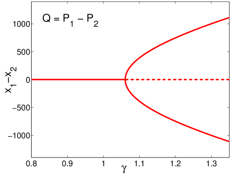
Figure 4: The dependence of steady state values of the symmetric variable $s=x_{1}-x_{2}$ on $\gamma$.

4.2 Stochastic Model I

To start our investigations in the equation-free framework, we constructed a very simple stochastic model of the system. We use this simple model to benchmark equation-free computations, since the results can be tested against Monte-Carlo simulations easily. Results for the full system are also presented below. The simple stochastic model consists only of reactions for the synthesis and degradation of proteins $P_{1}$ and $P_{2}$, but the following effective rate constants are used

$${\mbox{ \raise 3.69885pt\hbox{$\emptyset$}}}\quad\;\mathop{\stackrel{{\scriptstyle\mbox{\Large$\longrightarrow$}}}{{\mbox{\Large$\longleftarrow$}}}}^{\frac{1}{1+\kappa P_{1}}\frac{\gamma}{1+\omega P_{2}^{2}}}_{\frac{\delta}{1+\kappa P_{1}}}\quad{\mbox{ \raise 3.69885pt\hbox{$P_{1}$}}}$$ (4.7)

$${\mbox{ \raise 3.69885pt\hbox{$\emptyset$}}}\quad\;\mathop{\stackrel{{\scriptstyle\mbox{\Large$\longrightarrow$}}}{{\mbox{\Large$\longleftarrow$}}}}^{\frac{1}{1+\kappa P_{2}}\frac{\gamma}{1+\omega P_{1}^{2}}}_{\frac{\delta}{1+\kappa P_{2}}}\quad{\mbox{ \raise 3.69885pt\hbox{$P_{2}$}}}$$ (4.8)

The above reactions are consistent with the deterministic model, but in general do not preserve the noise structure of the full stochastic model.

To simulate the mechanism contained in model (4.7) – (4.8), we use the standard Gillespie SSA [13]. The results for different values of the parameter $\gamma$ are plotted in Figure 5.

$\gamma=0.8$

 

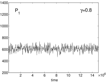
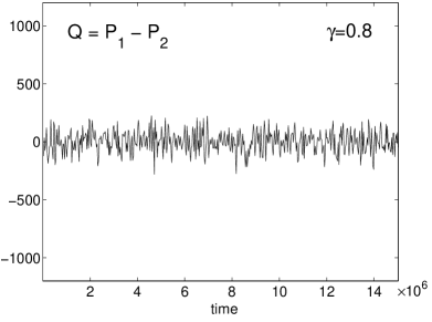
$\gamma=1.06$

 

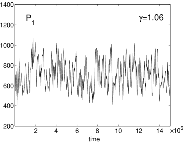
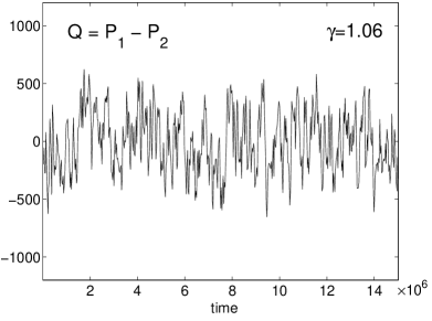
$\gamma=1.14$

 

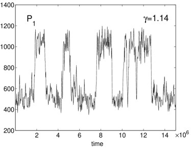
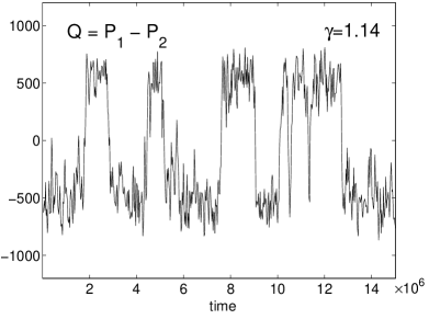
Figure 5: Stochastic Model I. Plots of $P_{1}$ and $Q=P_{1}-P_{2}$ as a function of time for different values of $\gamma.$ The parameter values used to produce these figures are $\delta=0.00075$, $\omega=2\times 10^{-6}$, and $\kappa=2\times 10^{-4}$.

For each $\gamma$ we plot the time evolution $P_{1}$ (left panel) and $Q=P_{1}-P_{2}$ (right panel). We see that for small $\gamma$, the solution fluctuates around the stable deterministic steady state with relatively small noise amplitude. When $\gamma=1.06$, the noise amplitude has increased substantially, which is typical of stochastic systems near a “bifurcation”; the word bifurcation is put here in quotes to denote that (in contrast to the deterministic case) there is no isolated parameter value marking the onset of bistability - no clear bifurcation point exists for the stochastic dynamics. Yet one can still claim that a clear bifurcation point exists for the critical points of the potential $\Phi(q,\gamma)$ in the stochastic model; furthermore, depending on the time horizon of our observation of a stochastic simulation, one may still appear to see an apparent bifurcation point for its averaged statistics (see the discussion in [16, 3]). If $\gamma$ is increased further, then $Q=0$ is no longer a stable steady state and the system clearly shows bistability. All plots are computed for the same time interval $[0,15\times 10^{6}].$ For $\gamma=1.25$ the steady states are sufficiently stable so that no transitions occurred in this time interval (data not shown). Therefore, for this case, determining the steady state probability distribution from long-term Monte-Carlo simulations would be very time consuming.

4.3 Stochastic Model II

Stochastic Model I considers only two variables $P_{1}$ and $P_{2}$. Here, we introduce a stochastic model that also takes into account the biochemical states of the operators, while maintaining the assumption that the dimerization reactions (2.3) – (2.4) are at equilibrium. That is, we consider the four variables $P_{1}$, $P_{2}$, $O_{1}$ and $O_{2}$. The model is defined in terms of the following reaction steps:

$${\mbox{\raise 3.69885pt\hbox{$\emptyset$}}}\quad\mathop{\stackrel{{\scriptstyle\mbox{ $\longrightarrow$}}}{{\mbox{ $\longleftarrow$}}}}^{\frac{\gamma}{1+\kappa P_{1}}\,O_{1}}_{\frac{\delta}{1+\kappa P_{1}}}\quad{\mbox{ \raise 3.69885pt\hbox{$P_{1}$}}}$$ (4.9)

$${\mbox{ \raise 3.69885pt\hbox{$\emptyset$}}}\quad\mathop{\stackrel{{\scriptstyle\mbox{ $\longrightarrow$}}}{{\mbox{ $\longleftarrow$}}}}^{\frac{\gamma}{1+\kappa P_{2}}\,O_{2}}_{\frac{\delta}{1+\kappa P_{2}}}\quad{\mbox{ \raise 3.69885pt\hbox{$P_{2}$}}}$$ (4.10)

$${\mbox{ \raise 3.69885pt\hbox{``$O_{1}=0$"}}}\quad\mathop{\stackrel{{\scriptstyle\mbox{ $\longrightarrow$}}}{{\mbox{ $\longleftarrow$}}}}^{K}_{K\omega P_{2}^{2}}\quad{\mbox{\raise 3.69885pt\hbox{``$O_{1}=1$"}}}$$ (4.11)

$${\mbox{ \raise 3.69885pt\hbox{``$O_{2}=0$"}}}\quad\mathop{\stackrel{{\scriptstyle\mbox{ $\longrightarrow$}}}{{\mbox{ $\longleftarrow$}}}}^{K}_{K\omega P_{1}^{2}}\quad{\mbox{ \raise 3.69885pt\hbox{``$O_{2}=1$"}}}$$ (4.12)

and contains an extra parameter, $K\equiv k_{-o1}=k_{-o2}$. Note that “$O_{1}=0$” means that the operator $O_{1}$ has a dimer of $P_{2}$ bound to it and therefore is “off” and “$O_{1}=1$” means that the operator $O_{1}$ is empty and therefore “on”. The same is true for $O_{2}.$ This implies that the random variables $O_{1}$ and $O_{2}$ are binary, whereas the variables $P_{1}$ and $P_{2}$ can take on any non-negative integer value. Stochastic Model I is recovered from Stochastic Model II in the limit $K\to\infty.$ We thus expect the models to produce similar results for large values of $K.$

Again, we use the standard Gillespie SSA [13] to simulate model (4.9) – (4.12). The results for different values of $K$ for $\gamma=1.14$ are plotted in Figure 6.

$K=0.1$, $\gamma=1.14$

 

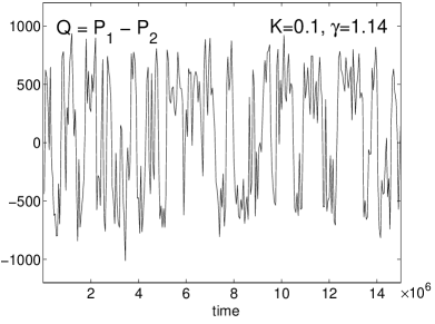
$K=1$, $\gamma=1.14$

 

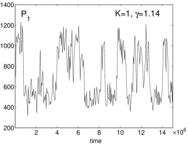
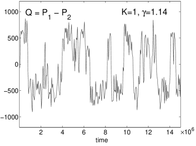
$K=10$, $\gamma=1.14$

 

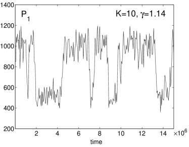
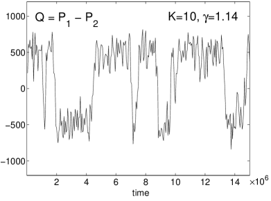
Figure 6: Stochastic Model II. Plots of $P_{1}$ and $Q=P_{1}-P_{2}$ as a function of time for different values of $K$ and $\gamma=1.14.$ The other model parameter values are the same as in Figure 5.

Comparing Figure 6 and corresponding panel from Figure 5, we can confirm that Stochastic Model II produces the same behavior as Stochastic Model I for large $K.$ However, in general, different values of $K$ can change the bifurcation structure of the system and affect the first passage times between the two stable steady states of the bistable system [23].

Because Stochastic Models I and II do not explicitly take into account dimerization, which in general is a fast process, they run much more efficiently than the full model given by (2.1) – (2.6). However, they do not in general preserve the noise structure of the full system. In the next section we use all three models to highlight the computational features (and potential benefits) of equation-free analysis.

5 Results of Equation-Free Analysis

In our approach, we want to study the stochastic models presented above using only short bursts of appropriately initialized stochastic simulations; the goal is to design these bursts, and process their results so as to determine long-time properties of the system (e.g., steady-state distributions, bifurcations, mean first passage times) efficiently. We use (and compare) the different algorithms discussed in Section 3.

5.1 The effective potential and steady state distribution

In this section, we use equation-free analysis to evaluate the effective potential (an “effective free energy”) and the steady-state distribution for Stochastic Models I and II and the full system. We start with Stochastic Model I. First, we will consider the slow variable $Q\equiv P_{1}-P_{2}$ and the fast (slaved) variable $R\equiv P_{1}+P_{2}.$ Initially the preparatory step (A) of the algorithm presented in Section 3 was done using the method outlined in (A1), i.e. we used the conditional mean $<\!\!R|Q=q\!\!>$ to initialize the computations in the step (B). A good approximation to this average can be found using the deterministic equations, and this was the number used in our preliminary computations to initialize the simulations in the step (B). That is, for a given $Q$, we initialized all realizations in the step (B) with the same value of $R$. Then we chose $\Delta t$ equal to 100 time steps of the Gillespie SSA. Note that this implies that the actual value of $\Delta t$ varies for each realization and depends on the values of the rate constants. However, the computer (CPU) time is the same for all the results presented for this case.

The equation-free results for the effective potential for different values of $\gamma$ are given in Figure 7.

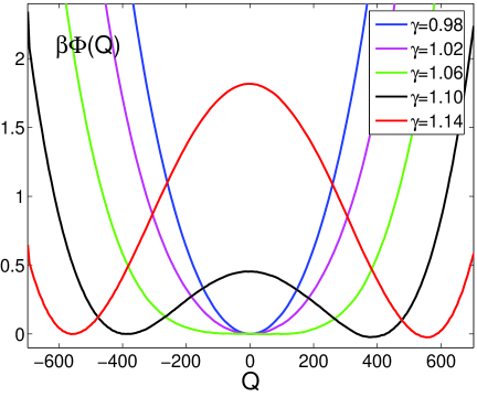
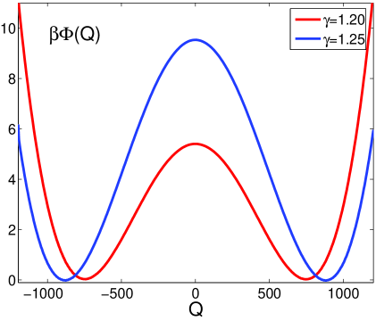
Figure 7: The effective free energy $\Phi$ for different values of $\gamma$ computed by our procedure. The other model parameter values are the same as in Figure 5.

These results are in good agreement with the long-term stochastic simulations presented in Section 4.2. The potential has a single minimum $\gamma<1.06$. As $\gamma$ is increased the potential broadens implying the system becomes “noisier”. When $\gamma>1.06$, the potential shows two local minima and the system is bistable.

Since we are using a very simple stochastic model, it is not computationally expensive to compute the steady-state distributions directly by long time simulations. We use the Gillespie SSA to generate $10^{11}$ time steps of the stochastic process and recorded the value of $Q$ at each time step. The resulting time series was binned to produce the steady-state distribution of the system. Figure 8 presents a comparison of the two computed steady state distributions. The results obtained by long-time simulations are shown as blue histograms and the steady state distributions computed from the effective potential $C\exp[-\beta\Phi(Q)]$ are given by the red lines.

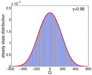
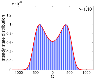
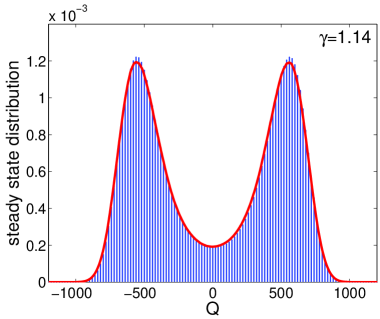
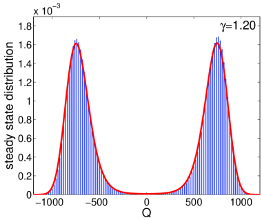
Figure 8: Comparison of steady state distributions obtained from the effective free energies shown in Figure 7 with histograms (blue) obtained by long time simulations.

We see that equation-free analysis gives very good results.

In Section 3, we introduced three possible methods, (A1) – (A3), to perform the preparatory step (A) (typically called the “lifting” step in the equation-free framework). We have shown that approach (A1) produces good results for Stochastic Model 1. Since (A1) works, there is no need to improve the results by considering (A2). Instead, we discuss the (A3) approach. In this approach given $Q=q$ we run the simulations for a short time $\delta t$ and record the value of $R$. Then we reset $Q=q$ but leave $R$ unchanged. We repeat this procedure many times and compute the conditional density $P(r|Q=q)$ as a histogram of recorded values of $R$. In our simulations, we chose $\delta t$ equal to one SSA step. To compute the conditional density $P(r|Q=q)$, we used 11 million SSA steps. First we let the system run for a million time steps to remove the transient in $R$, and then used remaining 10 million time steps to compute the conditional density. We used 200 million Gillespie time steps in part (B) of the algorithm. Consequently, step (A3) did not significantly change the computational cost of the program.

The graphs of $P(r|Q=q)$ for $\gamma=0.98$ and $\gamma=1.14$ are given in Figure 9. The left panel in these figures shows $P(r|Q=q)$ for five values of $Q$. The right panels show $P(r|Q=q)$ as a function of $r$ and $q$.

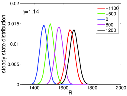
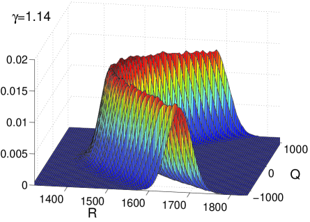
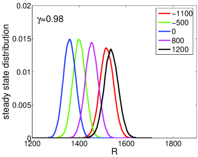
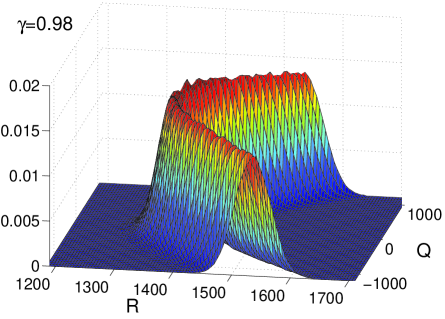
Figure 9: Conditional distribution $P(r|Q=q)$ for Stochastic Model I. Pictures on the left show $P(r|Q=q)$ for selected values of $q$. Pictures on the right show $P(r|Q=q)$ as a function of $r$ and $q$.

Next, we can use the computed conditional density $P(r|Q=q)$ to initialize $R$ in the step (B). Doing this, produces results which are virtually identical to results from Figure 8 (graphs not shown).

We now repeat the previous computations using the more complicated Stochastic Model II. The results are shown in Figures 10 and 11.

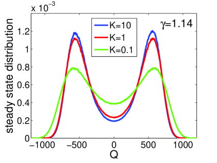
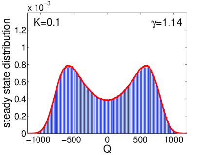
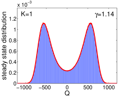
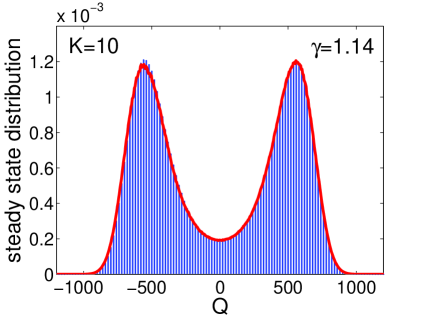
Figure 10: Comparison of steady state distributions from Stochastic Model II. The top left panel are results from the equation-free analysis for $K=0.1$, $K=1$ and $K=10$ and $\gamma=1.14$. The remaining three panels compare these results (red lines) to the steady state distribution computed from long-time Monte Carlo simulation (blue histograms). The other model parameter values are the same as in Figure 5.

In Figure 10, we choose $\gamma=1.14$ and compute the steady state distribution for $Q$ for three values of $K$. The results are compared with direct simulations of Stochastic Model II and with each other. The results from Figure 10 can also be compared to the corresponding plot with $\gamma=1.14$ in Figure 8, which can be viewed as the limit $K\to\infty.$ As can be seen, the results given by Stochastic Model II for $K=10$ are already in good agreement with the corresponding results obtained by Stochastic Model I. Figure 11 shows similar results for $\gamma=1.20$. Again, we obtained accurate results using the equation-free method.

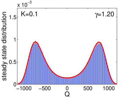
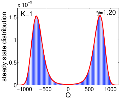
Figure 11: Stochastic Model II. Comparison of steady state distributions obtained by equation-free analysis (red line) with histograms (blue) obtained by long time stochastic simulations. In this figure $\gamma=1.2$ and $K=0.1$ in the left panel and $K=1$ in the right. The other model parameter values are the same as in Figure 5.

Up to now we have used the symmetric variable $Q\equiv P_{1}-P_{2}$ as our observable. However, we often do not have a priori knowledge of the slow variable, or, more generally, of a good observable to parametrize the long-time system dynamics. To investigate the sensitivity of our results to the choice of observable, we repeated the computations on Stochastic Model I using $P_{1}$ instead of $Q$. To use $P_{1}$ as our observable, we modify step (A1) so that we simply initialize $P_{2}$ using $P_{2}=\frac{1}{\delta}\frac{\gamma}{1+\omega P_{1}^{2}}.$ The numerical results for different values of $\gamma$ are given in Figure 12. Again good agreement is seen between the equation-free method and the Monte-Carlo simulations. Because $P_{1}$ has both a slow and a fast component, this result illustrates that equation-free methods can be used even when the slow variable is unknown. An extensive discussion of this point in a deterministic context can be found in [11]: one does not necessarily need the correct slow variable – one needs an observable that parametrizes the slow manifold, a quantity in terms of which the slow manifold can be expressed as the graph of a function.

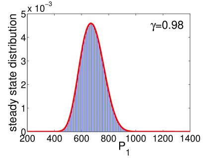
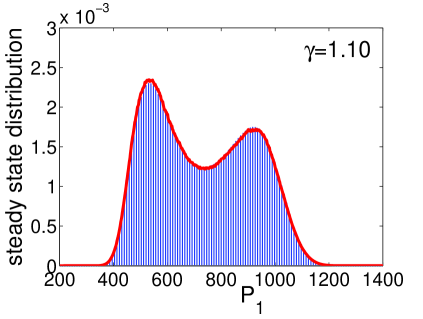
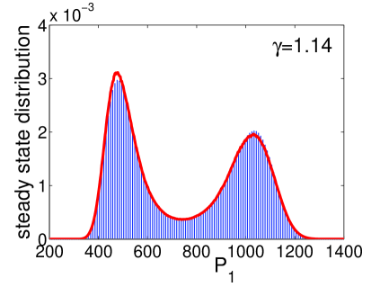
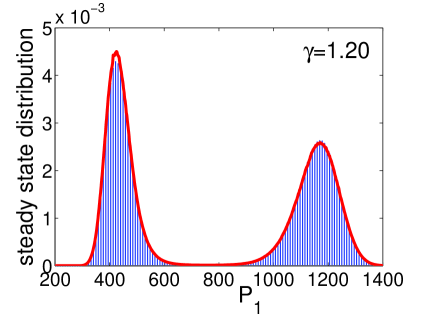
Figure 12: Comparison of steady state distributions using the variable $P_{1}$ as the observable for various values of $\gamma$. The other model parameter values are the same as in Figure 5. Again, the red lines are the results of equation-free analysis and the blue histograms are obtained by the long-time stochastic simulations.

Encouraged by the success of our computational framework for the simple Stochastic Models I and II considered above, we next investigated how well these methods would work on the full system described by equations (2.1) – (2.6). We first performed long time Monte Carlo simulations using BioNetS [1]. A two dimensional histogram for the total protein numbers $T_{1}=P_{1}+2\overline{P_{1}P_{1}}$ and $T_{2}=P_{2}+2\overline{P_{2}P_{2}}$ is shown in Figure 13(a). This simulation took over 500 total CPU hours and is the result of 800 runs distributed over 18 CPUs (over a trillion Gillespie SSA steps). The black curve in Figure 13(b) is the projection of the histogram onto the $T_{1}$ axis. We next performed equation-free computations for the system. As our single observable, $Q$, we used the total protein number $T_{1}$, because this is a quantity that can be measured using single cell fluorescent techniques. We used a slightly modified version of step (A3) to compute the conditional density $P({\bf r}|T_{1}=t_{1})$. For a given value of $T_{1}$, we set the rate constants for synthesis and degradation of this protein equal to zero. We then ran the simulations for a time of $1\times 10^{5}$ to remove any transients. Next still keeping $T_{1}$ fixed, $10000$ samples of the other variables were collected at evenly space intervals over a time period of $2\times 10^{5}$ and used to generate the conditional density. A time step of $\Delta t=15$ was used in step (B) of the algorithm. To compute the steady state distribution, polynomials were fit to the average velocity and effective diffusion coefficient computed from the equation-free analysis and then used to compute the effective free energy. The red curve shown in Figure 13(b) is the result of the equation-free analysis. It took less than an hour of CPU time. Very good agreement between the equation-free method and Monte Carlo simulation is seen. Our investigations into these methods revealed that whereas the velocity, $V(q)$, is robust to changes in $\Delta t$, the effective diffusion coefficient, $D(q)$, is quite sensitive and needs to be treated with care. Also, because of the exponential in the integral for the effective potential, small changes in the average velocity or effective diffusion coefficient can have large effects on the steady state distribution. Therefore, it is important to average over sufficiently many realizations to ensure convergence of average velocity and effective diffusion coefficient. Better estimation techniques, such as those developed by Aït-Sahalia using maximum likelihood [2] should be incorporated in the data processing step of the algorithms. Even with these caveats, the results presented in this section demonstrate the feasibility and high potential of equation-free methods for analyzing stochastic models of genetic networks.

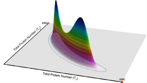
(a)   (b)

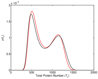
Figure 13: (a) The steady-state distribution for the total protein numbers computed from long-time Monte Carlo simulations of the full model $(\ref{prodP1})$ – $(\ref{onoffO2})$. (b) The projection of the 2D distribution onto the $T_{1}$ axis (black curve). The red curve is the result of the equation-free analysis. The parameter values used to compute these figures are $\gamma_{1}=\gamma_{2}=1.14$, $\delta_{1}=\delta_{2}=7.5\times 10^{4}$, $\epsilon_{1}=\epsilon_{2}=0,$ $k_{1}=k_{2}=5\times 10^{-4}$, $k_{-1}=k_{-2}=1$, $k_{o1}=k_{o2}=0.004$ and $k_{-o1}=k_{-02}=0.1$. These values are consistent with the parameter values $K=0.1$, $\delta=7.5\times 10^{4}$ and $\omega=2\times 10^{-6}$ used in Stochastic Models I and II.

5.2 First Passage Time

When $\gamma$ is sufficiently large the system is bistable. An important characterization of bistable systems is the average time for noise-induced transitions between the stable states. Here we make use of the definition of the first passage time from Section 3.2. For the results presented in this section we use $Q=P_{1}-P_{2}$ as our observable and Stochastic Model I. The system is bistable for $\gamma>1.06$. Let the deterministic stable steady states of $P_{1}$ be denoted as $p_{m}$ and $p_{M}$ with $p_{m}<p_{M}.$ Because of the symmetry of our problem, $p_{m}$ and $p_{M}$ are also the stable steady states of $P_{2}.$ Let the random variable ${\cal T}_{e}$ be defined as the first time when “$P_{1}=P_{2}$” given the initial conditions $P_{1}=p_{m}$ and $P_{2}=p_{M}.$ In terms of $Q$, this means that ${\cal T}_{e}$ denotes the time to reach $Q=0$ when the process starts with $Q$ equal to the negative steady state $q_{m}\equiv p_{m}-p_{M}$. Let $\tau_{e}$ denote the average of ${\cal T}_{e}$. Then, direct Monte Carlo simulations can be used to compute the value of $\tau_{e}.$ The results of such simulations for three different values of $\gamma$ are presented in the Table 1.

$\gamma$ $p_{m}$ $p_{M}$ $q_{m}=p_{m}-p_{M}$ computed $\tau_{e}$ from simulations $N$ 1.14 481.1 1038.6 -557.5 $7.0\times 10^{5}\pm 6.7\times 10^{3}$ 10 000 1.20 425.8 1174.2 -748.4 $1.6\times 10^{7}\pm 1.6\times 10^{5}$ 10 000 1.25 392.4 1274.3 -881.9 $1.0\times 10^{9}\pm 6.3\times 10^{7}$ 250

Table 1: The mean first passage time computed from long-time stochastic simulations, averaging over $N$ transitions. The results are expressed in the form ([sample mean] $\pm$ [sample variance]$/\sqrt{N}$).

As expected, the computational time needed to compute the mean first passage time increases rapidly with $\gamma$. In Section 3.2, we introduced two formulas (3.6) and (3.7) to compute $\tau_{e}$. Both formulas make use of the effective free energy computed by the equation-free algorithm. These potentials for $\gamma=1.14$, $\gamma=1.20$ and $\gamma=1.25$ are given in Figure 7. Consequently, we can compare the results obtained by the long simulations with the results found from formulas (3.6) and (3.7) for $\tau_{e;p}$ and $\tau_{e;k},$ respectively. The results are shown in Table 2.

$\gamma$ $\tau_{e}$ from Table 1 $\tau_{e;p}$ given by (3.6) $\tau_{e;k}$ given by (3.7) 1.14 $7.0\times 10^{5}$ $6.1\times 10^{5}$ $1.3\times 10^{6}$ 1.20 $1.6\times 10^{7}$ $1.4\times 10^{7}$ $2.6\times 10^{7}$ 1.25 $1.0\times 10^{9}$ $6.7\times 10^{8}$ $1.2\times 10^{9}$

Table 2: Comparison of the mean first passage time computed from equation-free analysis with long-time stochastic simulations.

Not surprisingly, the results given by $\tau_{e;p}$ are better than results given by the Kramers’ approximation $\tau_{e;k}$. However both methods produce results that are within a factor of 2 of the waiting times estimated from Monte Carlo simulations. As $\gamma$ becomes large the Monte Carlo simulations become computationally expensive. Therefore only $250$ realizations were used to estimate the mean first passage time, and we expect that the discrepancy between the Monte Carlo simulations and equation-free analysis for this case is due to finite sampling errors. Initializing the simulation at conditions that are rarely visited by the direct simulation itself constitutes a form of bias; this bias is designed to give faster computational estimates of the effective potential and – through this – of the first passage times. Clearly, this approach hinges on knowledge of a good observable, and in principle does not depend strongly on the value of the parameter $\gamma$; therefore, the larger the parameter $\gamma$ the higher the computational speedup in the first passage time estimation that will result. A quantitative study of this speedup is underway and will be reported elsewhere; it does not lie within the scope of this paper. We stress, however, that (as in molecular dynamics simulations) knowledge of a good observable (a good “reaction coordinate”) is crucial for the success of the approach.

Note that formula $\tau_{e;k}$ requires estimates of the second derivative of the potential at points $q_{u}$ and $q_{m}.$ To do this, we fit $\Phi(q)$ locally to a polynomial and used the derivatives of the polynomial at the required points; once again, maximum likelihood techniques (e.g. [2]) should be used for better results. The formula for $\tau_{e;p}$, requires the evaluation of an indefinite integral. The integral was approximated by considering only a finite interval that neglected contributions from the region of sufficiently small $q$ where the potential $\Phi$ is very large.

5.3 Bifurcations

In this section, our goal is to run the simulations for short times only and compute a form of “stochastic bifurcation diagram” using continuation methods, as an extension of the deterministic bifurcation computations. We use Stochastic Model I and study the dependence of the “steady states” on $\gamma$; the “steady states” we report are the fixed points of the algorithm from Section 3.1 with the conditional density $P(R|Q=q)$ approximated by the Dirac delta function in ($\mathbb{A}$) – ($\mathbb{B}$), similar to the approach (A1) from Section 3. Numerical results are given in Figure 14. For comparison we also plot

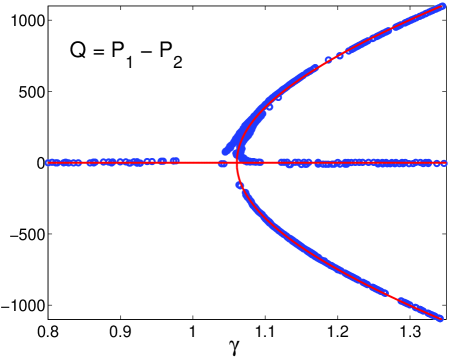
Figure 14: A plot of the steady states obtained by equation-free analysis $(\ref{numcont})$ (blue circles). Also shown are the deterministic steady states from Figure 4 (red line).

the steady states of the corresponding deterministic equation (compare with Figure 4). The plot in Figure 14 was computed by initializing on different branches far from the bifurcation point and continuing from these different initializations (our simple arclength continuation algorithm did not include a “pitchfork detection” component).

The accuracy of the numerical results depend on several factors: the estimation technique for the Jacobian elements, the tolerance of the error for Newton-Raphson iterations, the number of realizations which are used to evaluate $F$, the time interval $\Delta t$ and the steepness of the underlying potential $\Phi$. As can be seen in Figure 14, stochasticity along with all these numerical factors have slightly perturbed the pitchfork bifurcation; this could be exacerbated by our choice of (symmetric or asymmetric) observable. It is easy to follow any branch of steady states far from the bifurcation point. For obvious reasons this becomes more complicated when we are close to the “bifurcation point” at $\gamma=1.06$. The main problem is that the potential becomes “flat” close to the bifurcation point — see Figure 7. One way to improve the results is to adaptively change the number of realizations in ($\mathbb{B}$). That is, if the Newton-Raphson iterations of (3.5) do not converge to a desired tolerance, then more realizations are added. Another approach is to estimate directly a local polynomial model of the underlying diffusion process from discrete SSA data using maximum likelihood tools, and then search for the bifurcations of the critical points of the effective potential. Indeed, one can plot the zeroes of the estimated drift, or – in the case of a state-dependent diffusion coefficient – one can correct them to report the maxima of the steady state distribution [25, 37]; both of these are good candidate bifurcation diagrams for the stochastic case. When the potential is steep and the equilibrium is “less noisy” it is not necessary to use many realizations; the relation between computational effort (in terms of number of replicas, simulation time horizon and estimation method) and resulting accuracy is, again, a subject of current investigation beyond the scope of this paper.

Finally, the results using $P_{1}$ instead of $Q$ as the observable are shown in Figure 15.

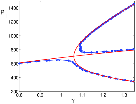
Figure 15: Plot of the steady states obtained by using $P_{1}$ as the observable (blue circles). Again for comparison the deterministic case is shown as the red line.

In this case, the asymmetry of our observable, and the perturbation it causes on the initialization process, make the perturbation of the pitchfork bifurcation stronger. Of course, the results depend on the initialization procedure, our estimation technique, the error tolerance, the number of realizations, the length of time step $\Delta t$ as well as the type of continuation algorithm we are using (here we used a very simple one, without bifurcation detection, in order to demonstrate what is possible). Accurate bifurcation detection depends on accurate Jacobians and even higher derivatives; estimating these from dynamic (and noisy !) data is notoriously difficult. While conceptually we do have the tools to “hone in” the more accurate detection of bifurcation points, careful quantitative work is necessary to pin down the tradeoffs between computational effort, model estimation accuracy and bifurcation point estimation accuracy.

6 Discussion

In this paper we discussed and illustrated the use of certain equation-free numerical techniques that have the potential to accelerate the computer-assisted analysis of stochastic models of regulatory networks. There is a clear current need for accelerating such simulations: even for modestly complex regulatory networks, stochastic models rapidly become computationally expensive. Computational acceleration is usually based on model reduction; theoretical methods for stochastic model reduction that take advantage of a separation of time scales are the focus of intense current research [23, 5, 17, 31, 34]. As we discussed in the introduction, many important gene regulatory networks do satisfy this assumption of a separation of time scales because synthesis and degradation of new proteins and transcripts usually occurs on a slower time scale than processes that change the chemical state of proteins. Analytical model reduction techniques assume that the fast variables are in quasi-steady state with respect to the slow variables, and use the quasi-steady state distributions conditioned on the slow variables to eliminate the fast variables by averaging. These methods have been successfully applied to simple models, but the theory is not as well established as the deterministic counterpart. Having an explicit model lies often at the basis of such stochastic reduction methods.

In the equation-free approach many of the same elements (separation of time scales, approximation of conditional quasi-steady distributions) also underpin computational efficiency; but the basic premise is that the model is available in the form of a “black box” simulation code. We do not try to first reduce, and then simulate the reduced surrogate; we try to design the smallest number of “intelligent” short computational experiments with the full stochastic model to find the quantities of interest, whether these are steady state probability distributions, their maxima, or transition rates in the bistable case. In that sense, the approaches we described here do not hinge upon the “inner”, detailed simulator as being a Gillespie SSA one - the methods are equally applicable to any “inner” simulator, stochastic or deterministic, as long as the main assumption of a low-dimensional effective stochastic model is a good one for the long-term system dynamics. Indeed, if another reduction method can be used to produce a good approximate dynamic simulator, our algorithms can be “wrapped” around this surrogate simulator rather than the full model for further acceleration.

Another important point has to do with the type of computation we are interested in - do we want to accelerate the direct simulation of the model, or do we want to accelerate the computation of certain features of its long-term dynamics (e.g. of the maxima of the steady state distribution)? These latter quantities can be also obtained from long-term direct simulation, but one of the points that we want to stress is that we can link direct simulation to different numerical algorithms (such as contraction mappings, and continuation methods) to obtain these quantities, often faster than with direct simulation alone. In the same way that bifurcation diagrams for dynamical systems are usually not computed through direct ODE integration, but through bifurcation algorithms, the parametric dependence of the long-term dynamics of stochastic models does not have to be computed through long-time direct simulation only. This “alternative” acceleration, not through accelerating the direct simulation itself, but through linking it to different numerical algorithms, lies at the basis of the equation-free framework.

Having said this, we briefly mention that equation-free methods for accelerating the direct simulation itself also exist. Coarse projective integration which uses short bursts of direct simulation to estimate time derivatives of evolving probability densities, and then passes them to standard numerical integration algorithms, has been successfully used in many contexts [24, 8, 10, 12] Coarse projective integration has a strong relation to the direct simulation acceleration methods in [15]; it has not been discussed in this paper, because we chose to focus on very long-term features of the network dynamics; it might interest the reader that the method can be used to also integrate backward in time, and solve “effective boundary value problems” to find “coarse” limit cycles [32].

In the equation-free methods for analyzing stochastic models of gene regulation that we discussed in this paper, we have tried to circumvent the difficulties encountered by direct simulation (in this case SSA) through the design of short bursts of appropriately initialized computational experiments with the full simulator. In a sense, we “resign ourselves” to the fact that the direct simulator is expensive; we ask what is the shortest amount of running of this expensive direct simulator in order to obtain the quantities we are interested in. The “design of experiment” protocols are templated on traditional continuum numerical methods, like the fixed point and continuation algorithms to compute bifurcation points, or quadrature to estimate Kramers’ formula. The only difference is that the quantities (residuals, actions of Jacobians, values of the integrand) that are required for numerical computation are not given by a closed formula, but rather through direct numerical simulation of the full model and estimation. We reiterate once more that these techniques can be wrapped around the full direct simulator, or our best available reduction of it, without change.

Knowing appropriate coarse-grained observables (the variables in terms of which the unavailable effective model would be written) is an important feature of the algorithms. Extensive experience with the problem, intuition, or analytical work may often suggest such observables; we did take advantage of such knowledge in this paper. We did already demonstrate an important point: more than one observables are capable of doing a good job as the parameterizing variables in an equation-free context; one does not need to know the exact slow variables. This issue is discussed extensively for the deterministic context in [11]. It is, however, important to note that algorithms for the detection of low-dimensionality in high-dimensional data can be vital in suggesting such observables from simulations. Principal Component Analysis is an established linear method for the detection of appropriate lower-order observables from simulation data; numerically estimated eigenmodes of the problem may also provide good observables (see the discussion in [36] about estimating gaps between eigenvalues, and using them to decide whether we should include more observables as independent variables). There are, however, some important developments in this area: the recent use of harmonic analysis (geometric diffusion) on graphs constructed from high-dimensional data shows great promise in detecting good observables (reaction coordinates) for complex, high dimensional systems [30, 4, 29]. This “variable-free” approach can be naturally linked to equation-free computation (one designs computational experiments both to detect the appropriate observables and to do computations with them) [30]; we are currently working on demonstrating this link for gene regulatory network modeling.

It is clear that, in certain cases, an equation-free computational approach is expected to have advantages over direct simulation. For steep potentials and low noise, for example, the way equation-free computation uses a good observable to bias the simulation will sample the effective potential and give a good estimate of the transition rates much faster than direct simulation. Also, parametric analysis methods should be able to explore parametric transitions faster and more systematically than direct simulation, in analogy with the use of bifurcation techniques rather than direct simulation in deterministic dynamical systems (e.g. by writing augmented algorithms that converge on marginally stable or unstable solutions). The complexity of the computation depends crucially on the dimensionality of the unavailable reduced model, and not so crucially on the dimensionality of the detailed, full model. We are currently working on the quantification of these computational benefits; this work is complicated by the fact that – lacking explicit formulas from which to obtain derivative information – errors must be computed on-line, through a posteriori estimates.

This brings us to a final, yet vital issue: estimation. Given the noisy nature of the data, estimating the numerical quantities of interest lies at the heart of the accuracy (and thus the viability) of the computation. For our gene networks, these quantities included the effective potential $\Phi(q)$ and the effective diffusion coefficient $D(q)$. Preliminary investigations revealed that the effective diffusion coefficient, $D(q)$, is quite sensitive to the time step $\Delta t$ and needs to be treated with care. Also, small changes in the average velocity or effective diffusion coefficient can have relatively large effects on the steady state distribution. Even though some computations are “embarrassingly parallel” (one short, fine scale realization per processor, running independently) variance reduction becomes an important feature (see, e.g. [28]). Maximum likelihood estimation techniques (e.g. [2]) take the place of simple formulas such as (3.2) and (3.3); one can envision certain hypothesis testing computations (is our model locally well-approximated by a diffusion process ?) becoming part of the overall computational scheme. Until these elements, and their computational cost, are analyzed and tested, there will be no firm guarantees for the computational efficiency of equation-free methods. Yet, even with these caveats, as we computationally demonstrated in this paper, we believe that the equation-free framework provides a promising new approach to gene regulatory network modeling, alternative to long-direct simulation. It links directly with powerful and tested traditional continuum numerical algorithms (such as numerical integration, fixed point algorithms, matrix-free iterative linear algebra) and with system theory techniques like filtering and estimation. These techniques are, in some sense “off the shelf” and do not need to be redeveloped. In our opinion, it is the linking of equation-free techniques with novel data reduction/clustering techniques (such as the use of the graph Laplacian to detect good reaction coordinates [30]) that hold the most promise in the computational study of complicated stochastic systems in general, and of gene regulatory networks and their models in particular.

Acknowledgments. This work was partially supported by DARPA and an NSF/ITR grant (I.G.K). This work was partially supported by Biotechnology and Biological Sciences Research Council (R.E.). This work was supported by DARPA (F30602-01-2-0579) (T.C.E.).

References

- [1] D. Adalsteinsson, D. McMillen, and T. Elston, Biochemical network stochastic simulator (BioNetS): software for stochastic modeling of biochemical networks, BMC Bioinformatics 5 (2004), no. 24, 1–21.
- [2] Y. Aït-Sahalia, Maximum-likelihood estimation of discretely-sampled diffusions: A closed-form approximation approach, Econometrica 70 (2002), 223–262.
- [3] D. Barkley, I. Kevrekidis, and A. Stuart, The moment map: Nonlinear dynamics of density evolution via a few moments, submitted to SIAM Journal on Applied Dynamical Systems, 2005.
- [4] M. Belkin and P. Niyogi, Laplacian eigenmaps for dimensionality reduction and data representation, Neural Computation 15 (2003), no. 6, 1373–1396.
- [5] Y. Cao, D. Gillespie, and L. Petzold, The slow-scale stochastic simulation algorithm, Journal of Chemical Physics 122 (2005), 14116.
- [6] E. Doedel, H. Keller, and J. Kernevez, Numerical analysis and control of bifurcation problems, part i, Int. J. Bifurcation and Chaos 1 (1991), no. 3, 493–520.
- [7] , Numerical analysis and control of bifurcation problems, part ii, Int. J. Bifurcation and Chaos 1 (1991), no. 4, 745–772.
- [8] R. Erban, I. Kevrekidis, and H. Othmer, An equation-free computational approach for extracting population-level behavior from individual-based models of biological dispersal, submitted to Physica D, 28 pages, 2004.
- [9] T. Gardner, C. Cantor, and J. Collins, Construction of a genetic toggle switch in e. coli, Nature 403 (2000), 339–342.
- [10] C. Gear, Projective integration methods for distributions, NEC TR 2001-130 (2001), 1–9.
- [11] C. Gear, T. Kaper, I. Kevrekidis, and A. Zagaris, Projecting on a slow manifold: Singularly perturbed systems and legacy codes, submitted to SIAM Journal on Applied Dynamical Systems, can be found as Physics/0405074 at arXiv.org, 2004.
- [12] C. Gear, I. Kevrekidis, and C. Theodoropoulos, ’Coarse’ integration/bifurcation analysis via microscopic simulators: micro-Galerkin methods, Computers and Chemical Engineering 26 (2002), no. 4, 941–963.
- [13] D. Gillespie, Exact stochastic simulation of coupled chemical reactions, The journal of physical chemistry 81 (1977), no. 25, 2340–2361.
- [14] , Markov Processes, an introduction for physical scientists, Academic Press, Inc., Harcourt Brace Jovanowich, 1992.
- [15] , Approximate accelerated stochastic simulation of chemically reacting systems, The journal of chemical physics 115 (2001), no. 4, 1716–1733.
- [16] M. Haataja, D. Srolovitz, and I. Kevrekidis, Apparent hysteresis in a driven system with self-organized drag, Physical Review Letters 92 (2004), no. 16, 160603.
- [17] E. Haseltine and J. Rawlings, Approximate simulation of coupled fast and slow reactions for stochastic chemical kinetics, Journal of Chemical Physics 117 (2002), 6959–6969.
- [18] J. Hasty, D. McMillen, and J. Collins, Engineered gene circuits, Nature 420 (2002), 224–230.
- [19] J. Hasty, D. McMillen, F. Isaacs, and J. Collins, Computational studies of gene regulatory networks: in numero molecular biology, Nature Reviews Genetics 2 (2001), 268–279.
- [20] G. Hummer and I. Kevrekidis, Coarse molecular dynamics of a peptide fragment: free energy, kinetics and long time dynamics computations, Journal of Chemical Physics 118 (2003), no. 23, 10762–10773.
- [21] M. Kaern, T. Elston, W. Blake, and J. Collins, Stochasticity in gene expression: from theories to phenotypes, Nature Reviews Genetics 6 (2005), 451–464.
- [22] C. Kelley, Solving nonlinear equations with newtons method, SIAM, 2003.
- [23] T. Kepler and T. Elston, Stochasticity in transcriptional regulation: Origins, consequences and mathematical representations, Biophysical Journal 81 (2001), 3116–3136.
- [24] I. Kevrekidis, C. Gear, J. Hyman, P. Kevrekidis, O. Runborg, and K. Theodoropoulos, Equation-free, coarse-grained multiscale computation: enabling microscopic simulators to perform system-level analysis, Communications in Mathematical Sciences 1 (2003), no. 4, 715–762.
- [25] D. Kopelevich, A. Panagiotopoulos, and I. Kevrekidis, Coarse-grained kinetic computations of rare events: application to micelle formation, Journal of Chemical Physics 122 (2005), 044908.
- [26] A. Makeev, D. Maroudas, and I. Kevrekidis, ”Coarse” stability and bifurcation analysis using stochastic simulators: Kinetic Monte Carlo examples, The Journal of Chemical Physics 116 (2002), no. 23, 10083–10091.
- [27] A. Makeev, D. Maroudas, A. Panagiotopoulos, and I. Kevrekidis, Coarse bifurcation analysis of kinetic monte carlo simulations: a lattice gas model with lateral interactions, The Journal of Chemical Physics 117 (2002), no. 18, 8229–8240.
- [28] M. Melchior and H.C. Öttinger, Variance reduced simulations of stochastic differential equations, Journal of Chemical Physics 103 (1995), 9506–9509.
- [29] B. Nadler, S. Lafon, R. Coifman, and I. Kevrekidis, Diffusion maps, spectral clustering and eigenfunctions of fokker-planck operators, can be found as Math/0506090 at arXiv.org, 2005.
- [30] , Diffusion maps, spectral clustering and the reaction coordinates of dynamical systems, to appear in Appl. Comp. Harm. Anal., 2005.
- [31] C. Rao and A. Arkin, Stochastic chemical kinetics and the quasi-steady-state assumption: application to the gillespie algorithm, Journal of Chemical Physics 118 (2003), 4999–5010.
- [32] R. Rico-Martinez, C. Gear, and I. Kevrekidis, Coarse projective kMC integration: Forward/reverse initial and boundary value problems, Journal of Computational Physics 196 (2004), no. 2, 474–489.
- [33] H. Risken, The Fokker-Planck Equation, methods of solution and applications, Springer-Verlag, 1989.
- [34] H. Salis and Y. Kaznessis, Accurate hybrid stochastic simulation of a system of coupled chemical or biochemical reactions, The Journal of Chemical Physics 122 (2005), 054103.
- [35] T. Schlitt and A. Brazma, Modelling gene networks at different organisational levels, FEBS Letters 579 (2005), 1859–1866.
- [36] C. Siettos, M. Graham, and I. Kevrekidis, Coarse Brownian dynamics for nematic liquid crystals: Bifurcation, projective integration, and control via stochastic simulation, Journal of Chemical Physics 118 (2003), no. 22, 10149–10156.
- [37] S. Sriraman, I. Kevrekidis, and G. Hummer, Coarse nonlinear dynamics of filling-emptying transitions: water in carbon nanotubes, submitted to Physical Review Letters, 2005.