Recirculating BBU thresholds for polarized HOMs with optical coupling

Abstract

Here we will derive the general theory of the beam-breakup instability in recirculating linear accelerators with coupled beam optics and with polarized higher order dipole modes. The bunches do not have to be at the same RF phase during each recirculation turn. This is important for the description of energy recovery linacs (ERLs) where beam currents become very large and coupled optics are used on purpose to increase the threshold current. This theory can be used for the analysis of phase errors of recirculated bunches, and of errors in the optical coupling arrangement. It is shown how the threshold current for a given linac can be computed and a remarkable agreement with tracking data is demonstrated. The general formulas are then analyzed for several analytically solvable cases, which show: (a) Why different higher order modes (HOM) in one cavity can couple and cannot be considered individually, even when their frequencies are separated by much more than the resonance widths of the HOMs. For the Cornell ERL as an example, it is noted that optimum advantage of coupled optics is taken when the cavities are designed with an $x$-$y$ HOM frequency splitting of above 50MHz. The threshold current is then far above the design current of this accelerator. (b) How the $x$-$y$ coupling in the particle optics determines when modes can be considered separately. (c) That the increase of the threshold current obtainable by coupled optics and polarized modes diminishes roughly with the square root of the HOMs’ quality factors. Therefore the largest advantages are achieved with cavities that are not specifically designed to minimize these quality factors, e.g. by means of HOM absorbers. (d) How multiple-turn recirculation interferes with the threshold improvements obtained with a coupled optics. Furthermore, the orbit deviations produced by cavity misalignments are also generalized to coupled optics. It is shown that the BBU instability always occurs before the orbit excursion becomes very large.

I Introduction

In several applications of linear accelerators the charged particle beam passes through the accelerating structures more than once after being lead back to the entrance of the linac by a return loop. By this method the linac can either add energy to electrons several times, or it can recapture the energy of high energy electrons after they have already been used for experiments. The former technique is referred to as recirculating linac, the latter as energy recovery linac (ERL) Tigner65_01 .

ERLs have received attention in recent years since they have the potential to accelerator currents much larger than those of non-recovering linacs, and since they have the potential for providing emittances smaller than those in x-ray storage rings at similar energies and for similar beam currents. This is due to the fact that the emittances in an ERL can be as small as that of the electron source, if emittance increase during acceleration can be avoided.

Several laboratories have proposed high power ERLs for different purposes. Designs for light production with different parameter sets and various applications are being worked on by Cornell University CHESS01_03 ; ERL03_12 , Daresbury Pool03_01 , TJNAF Benson01_01 , JAERI Sawamura03_02 , Novosibirsk Kulipanov98_01 , and KEK Suwada02_01 . TJNAF has incorporated an ERL in its design of an electron–ion collider (EIC) Merminga02_01 for medium energy physics, while BNL is working on an ERL–based electron cooler Benzvi03_01 for the ions in the relativistic ion collider (RHIC). The work at TJNAF, JAERI and Novosibirsk is based on existing ERLs of relatively small scale. The first international ERL workshop with over 150 participants in early 2005 has also shown the large interest in ERLs that is prevalent in the accelerator community.

One important limitation to the current that can be accelerated in ERLs or recirculating linear accelerators in general is the regenerative beam-breakup (BBU) instability. The size and cost of all these new accelerators certainly requires a very detailed understanding of this limitation. In hoff04 we have described this theory for particle motion in one degree of freedom. Here we generalize this theory to two degrees of freedom, i.e. to accelerators with polarized HOMs and $x$-$y$ coupling of the particle optics.

For one degree of freedom, a theory of BBU instability in recirculating linacs, where the energy is not recovered but added in each pass through the linac, was presented in Bisognano87_01 . This original theory was additionally restricted to scenarios where the bunches of the different turns are in the linac at about the same accelerating RF phase, such as in the so-called continuous wave (CW) operation where every bucket is filled. Tracking simulations Krafft87_01 compared well with this theory. This theory determines above what threshold current $I_{\rm th}$ the transverse bunch position $x$ displays undamped oscillations in the presence of a higher order mode (HOM) with frequency $\omega_{\lambda}$. If there is only one higher order mode and one recirculation turn with a recirculation time $t_{r}$ in the linac, the following formula is obtained for $T_{12}\sin\omega_{\lambda}t_{r}<0$:

$$I_{\rm th}=-\frac{2c^{2}}{e(\frac{R}{Q})_{\lambda}Q_{\lambda}\omega_{\lambda}}\frac{1}{T_{12}^{*}\sin\omega_{\lambda}t_{r}}\ ,$$ (1)

where $c$ is the speed of light, $e$ is the elementary charge, $(R/Q)_{\lambda}Q_{\lambda}$ is the impedance (in units of $\Omega$) of the higher order mode driving the instability, $Q_{\lambda}$ is its quality factor. In the case of one degree of freedom, $T_{12}^{*}=T_{12}$ is the element of the transport matrix that relates initial transverse momentum $p_{x}$ before and $x$ after the recirculation loop. A corresponding formula had already been presented in Randbook . Occasionally, additional factors are found when this equation is stated Sereno94 ; Beard03_01 ; Merminga01_01 . But in hoff04 it has been shown that no such additional factors are required.

The beam transport element $T_{12}$ appears since a HOM produces a transverse momentum $p_{x}$ during the first pass of a particle. This produces a transverse position of $x=T_{12}p_{x}$ when the particle traverses the HOM for a second time, and this in turn excites the HOM itself by means of the wake field $Wx=WT_{12}p_{x}$.

When the mode is polarized with an angle $\theta$, the kick produced during the first turn corresponds to the momentum $(p_{x},p_{y})=p(\cos\theta,\sin\theta)$. With a coupled optics, the resulting orbit displacement when the particle reaches the HOM after the return loop is $\vec{x}=p(T_{12}\cos\theta+T_{14}\sin\theta,T_{32}\cos\theta+T_{34}\sin\theta)$. This excites the higher order mode by the projection of this displacement onto the wake field, $\vec{W}\cdot\vec{x}=Wp(T_{12}\cos^{2}\theta+(T_{14}+T_{32})\sin\theta\cos\theta+T_{34}\sin^{2}\theta)$.

The HOM therefore produces a transverse kick that feeds back to itself, exactly as in the case with one degree of freedom, only that $T_{12}$ needs to be replaced Pozdeyev05 by

$$T_{12}^{*}=T_{12}\cos^{2}\theta+(T_{14}+T_{32})\sin\theta\cos\theta+T_{34}\sin^{2}\theta\ .$$ (2)

While equation 1 is derived with one HOM, for one degree of freedom it is often a good approximation even when the cavity has several higher order modes. It was shown in hoff04 that different HOMs can be treated individually when their frequencies differ by more than about $\frac{\omega_{\lambda}}{2Q_{\lambda}}$. This statement does not hold for two degrees of freedom as will be shown in this paper. Modes cannot in general be treated independently, even when their frequencies are separated by much more than the width of the HOM’s resonance.

An optics configuration that makes $T_{12}^{*}$ close to zero in order to make the threshold current very large has been proposed Rand80 ; Tennant05 and tested for coupled beam transport and polarized HOMs. This is a good technique when there is one dominant HOM. When there are several modes this approach does not apply directly, even if these modes are separated by more than the width of their resonance.

The paper is arranged as following: first, a dispersion relation for the current $I_{0}(\omega)$ is derived including coupling in a one turn recirculating linac with one cavity having multiple polarized HOMs. The smallest real value of $I_{0}$ that can be obtained with real $\omega$ determines the threshold current. Analytical solutions are given for the case of two polarized HOMs in one cavity. It is explained how the dispersion relation for this simple case can be solved efficiently on a computer, and comparisons to analytical approximations are presented. Approximations are then given for $N$ polarized modes in one cavity. Subsequently a dispersion relation for multiple cavities and multiple recirculation loops is derived that can only be solved numerically with similarly efficient techniques. Finally, misalignments of cavities are considered to investigate when these misalignments lead to a very large static displacement of the beam orbit.

II $N$ polarized modes in one cavity

For simplicity we are here investigating one cavity with $N$ higher-order dipole modes (HOMs), each having a polarization angle $\theta_{\lambda}$ to the horizontal. Note that slightly polarized cavities often have at least two HOMs with similar characteristics, and looking at a single polarized HOM can therefore be misleading.

The unit vector in the direction of the polarization is $\vec{e}_{\lambda}=\cos\theta_{\lambda}\vec{e}_{x}+\sin\theta_{\lambda}\vec{e}_{y}$. The effective transverse voltage in each HOM is $V_{\lambda}$, so that a particle traversing this HOM obtains a transverse-momentum change of $\frac{e}{c}\vec{e}_{\lambda}V_{\lambda}$. When $\vec{V}$ is the vector of all these $N$ voltages, then the momentum change is

$$\Delta\vec{p}=\frac{e}{c}{\bf E}\vec{V}\ ,\ \ {\bf E}=\left(\begin{array}[]{ccc}\vec{e}_{1}\ldots\vec{e}_{N}\end{array}\right)\ .$$ (3)

When the particle returns to the cavity after the return time $t_{r}$, the particle’s position has changed by

$$\Delta\vec{x}(t^{\prime})={\bf T}\Delta\vec{p}(t^{\prime}-t_{r})\ ,\ \ {\bf T}=\left(\begin{array}[]{cc}T_{12}&T_{14}\\ T_{32}&T_{34}\end{array}\right)\ .$$ (4)

This position will increase the voltage in $V_{\lambda}(t)$ by the projection of the mode’s wake field $W_{\lambda}(t-t^{\prime})\vec{e}_{\lambda}$ onto $\Delta\vec{x}(t^{\prime})$ times the charge $I(t^{\prime})dt^{\prime}$ that excites the field, i.e. $I(t^{\prime})W_{\lambda}(t-t^{\prime})\vec{e}_{\lambda}\cdot\Delta\vec{x}(t^{\prime})dt^{\prime}$. Integrating over all contributions to the HOM potentials leads to

$$\vec{V}(t)=\frac{e}{c}\int_{-\infty}^{t}I(t^{\prime}){\bf W}(t-t^{\prime}){\bf D}\vec{V}(t^{\prime}-t_{r})dt^{\prime}$$ (5)

with

$${\bf W}={\rm diag}(W_{\lambda})\ ,\ \ {\bf D}={\bf E}^{T}\,{\bf T}\,{\bf E}$$ (6)

and therefore

$$D_{\mu\mu} = T_{12}\cos^{2}\theta_{\mu}+T_{34}\sin^{2}\theta_{\mu}+\frac{T_{32}+T_{14}}{2}\sin 2\theta_{\mu}\ ,$$

$$D_{\mu\nu} = T_{12}\cos\theta_{\mu}\cos\theta_{\nu}+T_{34}\sin\theta_{\mu}\sin\theta_{\nu}$$ (7)

$$+ T_{32}\sin\theta_{\mu}\cos\theta_{\nu}+T_{14}\cos\theta_{\mu}\sin\theta_{\nu}\ .$$

Here $I(t^{\prime})$ is the current of the bunches that have already traveled for one turn; in the approximation of short bunches it is given by

$$I(t)=I_{0}t_{b}\sum_{m=-\infty}^{\infty}\delta(t-t_{r}-mt_{b})\ .$$ (8)

This transforms the integral equation into

$$\vec{V}(t)=I_{0}\frac{e}{c}t_{b}\sum_{m=-\infty}^{\infty}{\bf W}(t-t_{r}-mt_{b}){\bf D}\vec{V}(mt_{b})$$ (9)

where $W_{\lambda}(t)=0$ for $t\leq 0$.

The Laplace transform of $\vec{V}(t)$ can be written as

$$\vec{V}(t+\delta t_{b})=\frac{1}{2\pi}\int_{-\infty-ic_{0}}^{\infty-ic_{0}}\vec{\tilde{V}}_{\delta}(\omega^{\prime})e^{-i\omega^{\prime}t}d\omega^{\prime}\ .$$ (10)

And with the following definition

$$\vec{\tilde{V}}^{\Sigma}_{\delta}(\omega)=\sum_{n=-\infty}^{\infty}\vec{\tilde{V}}_{\delta}(\omega+\frac{2\pi}{t_{b}}n)$$ (11)

one obtains

$$\vec{\tilde{V}}^{\Sigma}_{\delta}(\omega)=t_{b}\sum_{n=-\infty}^{\infty}\vec{V}([n+\delta]t_{b})e^{i\omega nt_{b}}\ .$$ (12)

Since $\vec{\tilde{V}}^{\Sigma}_{\delta}(\omega)$ is periodic with $2\pi/t_{b}$, it has a Fourier series, and its Fourier coefficients are $\vec{V}([n+\delta]t_{b})$, which shows that $\vec{\tilde{V}}^{\Sigma}_{\delta}(\omega)$ does not vanish. The transverse motion is stable when $\vec{\tilde{V}}(\omega)$ is zero for all $\omega$ with positive imaginary part. If the current is increased the motion can become unstable at which point $\vec{\tilde{V}}(\omega)$ is non-zero for at least one $\omega$ with positive imaginary part. At threshold it is therefore non-zero for a real value of $\omega$.

As in hoff04 we will use $t_{r}=(n_{r}-\delta)t_{b}$ to allow for all recirculating phases, e.g. $\delta=\frac{1}{2}$ for an ERL. The integral equation now leads to a relation for these coefficients,

$$I_{0}^{-1}\vec{V}^{\Sigma}_{0}(\omega)$$

$$= \frac{e}{c}t_{b}^{2}\sum_{m,n=-\infty}^{\infty}{\bf W}([n-n_{r}-m+\delta]t_{b}){\bf D}\vec{V}(mt_{b})e^{i\omega nt_{b}}$$

$$= \frac{e}{c}e^{i\omega n_{r}t_{b}}{\bf W}^{\Sigma}_{\delta}(\omega){\bf D}\vec{V}^{\Sigma}_{0}(\omega)\ .$$

This formulation shows that $\vec{V}^{\Sigma}_{0}(\omega)$ is an eigenvector of the matrix on the right-hand side, and the corresponding eigenvalue is $1/I_{0}$. Its solution is therefore very similar to the matrix theory for BBU computation without coupling in Bisognano87_01 . The threshold current can thus be determined by finding the largest real eigenvalue of this matrix for any real $\omega$. Due to the symmetry properties ${\bf W}^{\Sigma}_{\delta}(\omega+\frac{2\pi}{t_{b}})={\bf W}^{\Sigma}_{\delta}(\omega)$ and ${\bf W}^{\Sigma}_{\delta}(-\omega)={\bf W}^{\Sigma*}_{\delta}(\omega)$, it is sufficient to investigate $\omega\in[0,\pi/t_{b}]$ to find the BBU threshold current,

$$I_{th}^{-1}=\frac{e}{c}\max_{\omega\in[0,\pi/t_{b}]}\{\Lambda|e^{i\omega n_{r}t_{b}}{\bf W}^{\Sigma}_{\delta}(\omega){\bf D}\vec{V}=\Lambda\vec{V},\Lambda\in I\!\!R\}\ .$$ (14)

II.1 Two polarized HOMs in one cavity

For a large number of HOMs this equation should be solved numerically, but for two HOMs a analytical solution is simple. The characteristic polynomial for the eigenvalue $1/I_{0}$ becomes

$$\left|\left(\begin{array}[]{cc}\tilde{I}^{-1}-D_{11}w_{1}&-D_{12}w_{1}\\ -D_{21}w_{2}&\tilde{I}^{-1}-D_{22}w_{2}\end{array}\right)\right|=0\ ,$$ (15)

with $\tilde{I}=\frac{et_{b}}{c}e^{i\omega t_{r}}I_{0}$ and $w_{\lambda}=\frac{1}{t_{b}}e^{i\omega\delta t_{b}}({\bf W}^{\Sigma}_{\delta})_{\lambda\lambda}$. Solving this quadratic equation leads to

$$\frac{c}{et_{b}}e^{-i\omega t_{r}}I_{0}^{-1}=\frac{D_{11}w_{1}+D_{22}w_{2}}{2}$$ (16)

$$\pm\sqrt{(\frac{D_{11}w_{1}-D_{22}w_{2}}{2})^{2}+w_{1}w_{2}D_{12}D_{21}}\ .$$

To reduce the threshold current, the left hand side of this formula should be small.The matrix ${\bf D}$ is determined by the mode polarization and by the linear particle optics. It has been suggested Rand80 ; Pozdeyev05 to use these parameters to increase the threshold current. These suggestions amount to reducing the right hand side of Eq. (16) by making $D_{11}$ and $D_{22}$ small. This is always a valid strategy if there is only one HOM, i.e. $w_{2}=0$. Then

$$D_{11}=T_{12}\cos^{2}\theta_{1}+T_{34}\sin^{2}\theta_{1}+\frac{T_{14}+T_{32}}{2}\sin 2\theta_{1}$$ (17)

and a horizontally ($\theta_{1}=0$) or a vertically ($\theta_{1}=\frac{\pi}{2}$) polarized mode together with a beam transport that fully couples the vertical to the horizontal motion and vice versa, i.e. $T_{12}=T_{34}=0$, would always lead to $D_{11}=0$ so that there would not be any threshold current. A formula for this case has been derived in Pozdeyev05 .

For the case of two or more HOMs this method is no longer as effective, even when the modes have very different frequencies. In fact it has been suggested that in cases with several modes, each mode could be considered separately when each cavity mode has a resonance width which is significantly smaller than the frequency separation between modes Pozdeyev05 . This is however not correct and it will be seen shortly that the described method that would seem to increase the threshold current when all modes are considered separately is not as effective even when modes frequencies differ by much more than the resonance width. This is especially important when there are two HOMs of similar properties, for example in nearly cylindrically symmetric cavities. To see this effect, we distinguish three cases.

II.1.1 Circular symmetry

For circular symmetric cavities there are two equivalent modes with perpendicular polarization, $w_{1}=w_{2}$, $\vec{e}_{1}=\vec{e}_{x}$, $\vec{e}_{2}=\vec{e}_{y}$ leading to ${\bf D}={\bf T}$,

$$I_{0} = \frac{e}{ct_{b}}\frac{e^{-i(\omega t_{r}+\vartheta_{\pm})}}{T_{\pm}w_{1}}\ ,$$ (18)

$$T_{\pm}e^{i\vartheta_{\pm}} = \frac{T_{12}+T_{34}}{2}\pm\sqrt{(\frac{T_{12}-T_{34}}{2})^{2}+T_{14}T_{32}}\ ,$$

$${\rm with}\ T_{\pm}\in I\!\!R^{+}\ .$$

where the threshold current is the smaller of the two values obtained with the equation for $+$ and for $-$. For $T_{12}=T_{34}=0$ this case has been considered in Yunn05 . If there is no coupling, $T_{+}=|T_{12}|$ and $T_{-}=|T_{34}|$. This result is equivalent to what has been found in hoff04 for motion in one degree of freedom.

As in hoff04 we now use long range wake fields of the form

$$W_{\lambda}(\tau)=\left(\frac{R}{Q}\right)_{\lambda}\frac{\omega_{\lambda}^{2}}{2c}e^{-\frac{\omega_{\lambda}\tau}{2Q_{\lambda}}}\sin(\omega_{\lambda}\tau)\ ,$$ (19)

where $Q_{\lambda}$ is the quality factor, $\omega_{\lambda}$ is the frequency, and $(R/Q)_{\lambda}$ is the impedance in units of $\Omega$ for the linac definition (2 times the circuit definition). As shown in hoff04 , $|w_{\lambda}(\omega)|$ is especially large when $\omega$ is close to $\omega_{\lambda}$.

When motion in only one dimension is considered as in hoff04 , one obtains

$$I_{0}\approx\frac{c}{et_{b}}\frac{e^{-i\omega t_{r}}}{T_{12}w_{\lambda}}\ .$$ (20)

For simplicity we again use $\mathcal{K}_{\lambda}=t_{b}\frac{e\omega_{\lambda}^{2}}{2c^{2}}\left(\frac{R}{Q}\right)_{\lambda}$ and $\epsilon_{\lambda}=\frac{\omega_{\lambda}t_{b}}{2Q_{\lambda}}$. For $n_{r}\epsilon_{\lambda}\ll 1$ this leads to the approximation

$$I_{th} \approx \left\{\begin{array}[]{l}-\frac{2\epsilon_{\lambda}}{\mathcal{K}_{\lambda}}\frac{1}{T_{12}\sin(\omega_{\lambda}t_{r})}\ {\rm for}\ T_{12}\sin(\omega_{\lambda})<0,\\ \frac{2}{\mathcal{K}_{\lambda}|T_{12}|}\sqrt{\epsilon_{\lambda}^{2}+(\frac{\rm{mod}(\omega_{\lambda}t_{r},\pi)}{n_{r}})^{2}}\ {\rm else.}\end{array}\right.$$ (23)

For $\epsilon_{\lambda}\ll 1$ but $n_{r}\epsilon_{\lambda}\gg 1$ the approximation derived in hoff04 is

$$I_{th}\approx\frac{2\epsilon_{\lambda}}{\mathcal{K}_{\lambda}|T_{12}|}\ .$$ (24)

Exactly the same approximation and derivation therefore leads leads from Eq. (18) to

$$I_{th\pm} \approx \left\{\begin{array}[]{l}-\frac{2\epsilon_{\lambda}}{\mathcal{K}_{\lambda}}\frac{1}{T_{\pm}\sin(\omega_{\lambda}t_{r}+\vartheta_{\pm})}\ {\rm if\ it\ is}\ >0,\\ \frac{2}{\mathcal{K}_{\lambda}T_{\pm}}\sqrt{\epsilon_{\lambda}^{2}+(\frac{\rm{mod}(\omega_{\lambda}t_{r}+\vartheta_{\pm},\pi)}{n_{r}})^{2}}\ {\rm else.}\end{array}\right.$$ (27)

For $\epsilon_{\lambda}\ll 1$ but $n_{r}\epsilon_{\lambda}\gg 1$ the approximation derived in hoff04 is

$$I_{th\pm}\approx\frac{2\epsilon_{\lambda}}{\mathcal{K}_{\lambda}T_{\pm}}\ .$$ (28)

The threshold current is given by $I_{th}=\min_{\pm}(I_{th\pm})$.

To clarify the here considered case, we use typical parameters for the two HOMs: $Q_{1}=Q_{2}=10^{4}$, $\left(\frac{R}{Q}\right)_{1}=\left(\frac{R}{Q}\right)_{2}=100\Omega$, $\omega_{1}=\omega_{2}=2\pi\cdot 2.2$GHz, $t_{b}=1/1.3$GHz, $n_{r}-\delta=5.5$. For a decoupled optics with $T_{12}=-10^{-6}\frac{m}{eV/c}$, $T_{14}=T_{32}=0$ we obtain a threshold current of $I_{th}=46.40$mA that agrees to all specified digits when computed by particle tracking and by the approximation in Eq. (28). For a very much coupled beam transport (abbreviation $x=-10^{-6}\frac{m}{eV/c}$ is used below) the following threshold current is obtained:

$${\bf T}=\frac{1}{\sqrt{2}}\left(\begin{array}[]{cccc}1&x&1&3x\\ 0&1&0&1\\ -1&-2x&1&4x\\ 0&-1&0&1\end{array}\right)\ \Longrightarrow\ I_{th}=20.28{\rm mA}\ .$$ (29)

Again the threshold current computed by particle tracking and by Eq. (27) agree to all specified digits.

II.1.2 Small coupling

To cases with $|D_{11}w_{1}-D_{22}w_{2}|^{2}\gg|w_{1}w_{2}D_{12}D_{21}|$ we refer to it as small coupling. This denomination is motivated by the fact that when one mode is polarized in $x$ and one in $y$ direction, this case occurs when the optical coupling is small, as can be seen in Eq. (7). Equation (16) simplifies to

$$I_{0}=\frac{e}{ct_{b}}\frac{e^{-i\omega t_{r}}}{D_{\lambda\lambda}w_{\lambda}}\ ,$$ (30)

with $\lambda$ being either $1$ or $2$.

The approximation that leads from Eq. (20) to Eq. (23) can again be used and it leads to

$$I_{th}\approx-\frac{2\epsilon_{\lambda}}{\mathcal{K}_{\lambda}}\frac{1}{D_{\lambda\lambda}\sin(\omega_{\lambda}t_{r})}\ {\rm for}\ D_{\lambda\lambda}\sin(\omega_{\lambda}t_{r})<0\ ,$$ (31)

and similarly an approximation that corresponds to Eq. (24) is valid. This formula has been used to argue that an optics with very small $|D_{\lambda\lambda}|$ could be built with extremely large threshold current. But this equation does not apply when the $|D_{\lambda\lambda}|$ are too small, since then the following case has to be considered.

II.1.3 Strong coupling

To the case with $|D_{11}w_{1}-D_{22}w_{2}|^{2}\ll|w_{1}w_{2}D_{12}D_{21}|$ we refer to as strong coupling. This case is especially relevant when the mentioned coupling techniques have been used to make $D_{11}$ and $D_{22}$ very small. One obtains

$$I_{0}^{2}\approx(\frac{c}{et_{b}})^{2}\frac{e^{-i\omega 2t_{r}}}{w_{1}w_{2}D_{12}D_{21}}\ .$$ (32)

At the threshold current only one of the functions in the denominator will be very large and we call this $w_{\mu}$. The other mode will be indexed by $\nu$.

In hoff04 a first order approximation in $\Delta\omega t_{b}=(\omega-\omega_{\mu})t_{b}$ and $\epsilon_{\mu}$ is used to obtain Eqs. (23) and (24). Here we again expand to first order in these quantities, which is simple since $w_{\mu}^{-1}$ is linear in them so that $w_{\nu}^{-1}$ can be evaluated at $\Delta\omega=0$ and $\epsilon_{\nu}=0$, leading to

$$I_{0}^{2}\approx\frac{c}{et_{b}}\frac{e^{-i(\omega 2t_{r}+\vartheta)}}{Tw_{1}}\ .$$ (33)

With $Te^{i\vartheta}=\frac{et_{b}}{c}w_{\nu}(\omega_{\mu})D_{12}D_{21}$, $T\in I\!\!R^{+}$. Note that the exponent contains $2t_{r}$ instead of $t_{r}$. The approximations that correspond directly to Eqs. (27) and (28) can again be applied.

In hoff04 $w_{\lambda}$ is evaluated for the long-range wakefield, leading to

$$w_{\lambda} = \left(\frac{R}{Q}\right)_{\lambda}\frac{\omega_{\lambda}^{2}}{4c}$$

$$\times \frac{e^{i\omega^{+}(\delta-1)t_{b}}\sin(\omega_{\lambda}\delta t_{b})-e^{i\delta\omega^{+}t_{b}}\sin(\omega_{\lambda}[\delta-1]t_{b})}{\cos(\omega^{+}t_{b})-\cos(\omega_{\lambda}t_{b})}\ .$$

Note that here $w_{\lambda}$ is defined without a phase factor $e^{-i\omega\delta t_{b}}$ compared to hoff04 to simplify the notation. For an ERL, where $\delta=1/2$, one has

$$w_{\lambda}=\left(\frac{R}{Q}\right)_{\lambda}\frac{\omega_{\lambda}^{2}}{2c}\frac{\cos(\omega^{+}\frac{t_{b}}{2})\sin(\omega_{\lambda}\frac{t_{b}}{2})}{\cos\omega^{+}t_{b}-\cos\omega_{\lambda}t_{b}}\ ,$$ (35)

with $\omega^{+}t_{b}=\omega t_{b}+i\epsilon_{\lambda}$. Then $\omega=\omega_{\mu}+\Delta\omega$ with the small quantity $\Delta\omega t_{b}$. We assume that also $\epsilon_{\lambda}=\frac{\omega_{\lambda}t_{b}}{2Q_{\lambda}}$ is small, which is usually the case whenever BBU is relevant. A first order expansion in these small quantities leads to

$$I_{0}^{2}\approx\frac{2e^{-i\omega 2t_{r}}(\Delta\omega t_{b}+i\epsilon_{\mu})}{\mathcal{K}_{\mu}\mathcal{K}_{\nu}D_{12}D_{21}}\frac{\cos(\omega_{\mu}t_{b})-\cos(\omega_{\nu}t_{b})}{\cos(\omega_{\mu}\frac{t_{b}}{2})\sin(\omega_{\nu}\frac{t_{b}}{2})}\ .$$ (36)

If $I_{0}$ is the threshold current $I_{th}$, the right hand side has to be a real number, requiring $\Delta\omega t_{b}\sin(\omega 2t_{r})=\epsilon_{1}\cos(\omega 2t_{r})$. This leads to

$$I_{th\mu}^{2}\approx\frac{2\epsilon_{\mu}}{\mathcal{K}_{\mu}\mathcal{K}_{\nu}}\frac{\cos\omega_{\mu}t_{b}-\cos\omega_{\nu}t_{b}}{D_{12}D_{21}\cos(\omega_{\mu}\frac{t_{b}}{2})\sin(\omega_{\nu}\frac{t_{b}}{2})\sin(\omega_{\mu}2t_{r})}\ ,$$ (37)

whenever this term is positive. Whenever it is negative, the following approximation follows from hoff04 ,

$$I_{th\mu}^{2} \approx \frac{2}{\mathcal{K}_{\mu}\mathcal{K}_{\nu}}\left|\frac{\cos\omega_{\mu}t_{b}-\cos\omega_{\nu}t_{b}}{D_{12}D_{21}\cos(\omega_{\mu}\frac{t_{b}}{2})\sin(\omega_{\nu}\frac{t_{b}}{2})}\right|$$

$$\times \sqrt{\epsilon_{\mu}^{2}+(\frac{\mod(\omega_{\mu}2t_{r},\pi)}{2n_{r}})^{2}}\ .$$

For $\epsilon_{\mu}\ll 1$ but $n_{r}\epsilon_{\mu}\gg 1$ one obtains

$$I_{th\mu}^{2}\approx\frac{2\epsilon_{\mu}}{\mathcal{K}_{\mu}\mathcal{K}_{\nu}}\left|\frac{\cos\omega_{\mu}t_{b}-\cos\omega_{\nu}t_{b}}{D_{12}D_{21}\cos(\omega_{\mu}\frac{t_{b}}{2})\sin(\omega_{\nu}\frac{t_{b}}{2})}\right|\ .$$ (39)

These formulas are to be evaluated for $\mu=1$, $\nu=2$ and for $\mu=2$, $\nu=1$, and the smaller of the two resulting currents is the threshold current,

$$I_{th}=\min_{\mu\in\{1,2\}}\{I_{th\mu}\}\ .$$ (40)

An interesting observation is that for two modes with similar $Q_{\lambda}$, $\left(\frac{R}{Q}\right)_{\lambda}$, and $\omega_{\lambda}$, the ratio of the threshold current with and without coupled optics can be found by comparing Eqs. (37) and (31) and it is proportional to $\sqrt{1/\epsilon_{\lambda}}\propto\sqrt{Q_{\lambda}}$. For cavities that are optimized for large currents by means of sophisticated HOM damping, the advantage of a coupled optics therefore decreases. This effect is independent of the length of the return loop and is already relevant for a single cavity.

Figure 1 refers to a linac with one cavity and $t_{r}=555.5t_{b}$ that has two HOMs, one with $\omega_{1}=2.2$GHz polarized in $x$ and one with $\omega_{2}=2.3$GHz polarized in $y$ direction, $\left(\frac{R}{Q}\right)=100\Omega$, and $Q_{x}=Q_{y}$ is varied. The bottom data refer to a decoupled optics and the top data to a fully coupled optics with $T_{12}=0$ and $T_{34}=0$. A double-logarithmic plot is shown, which makes it apparent that the threshold current for a decoupled optics decreases with $Q^{-1}$, as indicated by the line with slope $-1$. A closer look shows that the slope is only accurately $-1$ for relatively small and relatively large $Q$ where either approximation 23 or 24 hold. A totally coupled optics with $T_{12}=0$ and $T_{34}=0$ leads to a larger threshold current than without coupling, but when $Q$ of the modes is reduced, the threshold current increases only with $Q^{-\frac{1}{2}}$ as indicated by a line with slope $-\frac{1}{2}$. The advantage of coupling decreases proportionally to $\sqrt{Q}$.

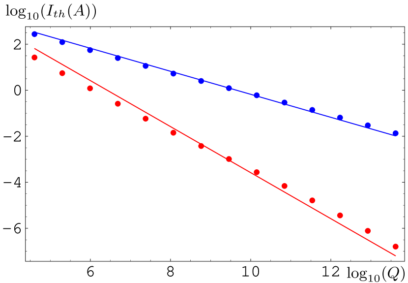
Figure 1: The threshold with two modes in one cavity scales with $Q^{-1}$ for a decoupled and with $Q^{-\frac{1}{2}}$ for a fully coupled optics. The advantage of coupling thus diminishes for low Q.

Figure 2 similarly shows the advantage of polarizing the higher order modes in the ERL that is proposed to upgrade the CESR ring at Cornell University erlpac05 . When the HOMs are polarized in $x$ and $y$ direction and the optics is completely coupled by $T_{12}=0$ and $T_{34}=0$, the threshold current is larger than without coupling, but again the advantage is smaller when the HOMs are damped more strongly by HOM absorbers. In fact, for the HOMs that are computed for $7$-cell cavities Liepe03 , the increase of the threshold current due to coupling is only a factor of $2.5$ as can be seen in Tab 1 when the HOM frequencies in $x$ and $y$ are separated by 10MHz. However, the figure shows that when many cavities are present, as in the ERL where there are 320, the scaling is not as simple as in the case of a single cavity and the advantage of coupling does not decrease as strongly with decreasing $Q$.

For Tab. 1 the 320 cavities of the ERL upgrade of CESR had nominal HOM frequencies of $f_{x}=1.87394$GHz with horizontal polarization. The mode with vertical polarization is $f_{y}=f_{x}-\Delta f_{xy}$. The cavities have HOM frequencies that have a Gaussian distribution around these values with rms width $\sigma_{RF}$. We used 500 different random distributions of the frequencies and display the average threshold current $I_{th}$ as well as the rms $\sigma_{I}$ of the 500 resulting thresholds. All modes have $\left(\frac{R}{Q}\right)=109.60\Omega$ and $Q=20912.4$.

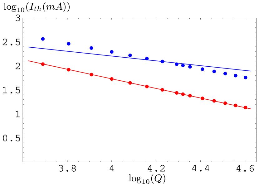
Figure 2: The threshold increase due to coupling of the x-ray ERL upgrade of CESR scales roughly with $\sqrt{Q}$.

Table 1: Threshold currents for the two most significant HOMs of the Cornell ERL.

$\Delta f_{xy}$	Coupling	$\sigma_{RF}$	$I_{th}$	$\sigma_{I}$
10MHz	NO	0MHz	25.8mA	0mA
10MHz	YES	0MHz	103mA	0mA
10MHz	NO	1.3MHz	280mA	43mA
10MHz	YES	1.3MHz	867mA	100mA
60MHz	NO	10MHz	418mA	69mA
60MHz	YES	10MHz	2420mA	433mA

II.2 Comments about numerical solutions

When the threshold current for two polarized modes at $\omega_{\nu}$ and $\omega_{\mu}$ should be found by solving Eqs. (30) and (32) numerically, the eigenvalues are plotted in the complex plain, and the intersections with the real axis are sought that lead to the smallest current. An example of the two eigenvalues plotted in the complex plain is shown in Fig. 3. The eigenvalues are largest in the vicinity of $\omega=|{\rm mod_{\pm}}(\omega_{\lambda},\frac{2\pi}{t_{b}})|$, $\lambda\in\{1,2\}$, since there either $w_{\mu}$ or $w_{\nu}$ become very large. The subscript on the mod function indicates that ${\rm mod_{+}}(x,1)\in[0,1]$ and ${\rm mod_{-}}(x,1)\in[-\frac{1}{2},\frac{1}{2}]$.

Furthermore, the eigenvalues trace out loops around the origin of the complex plain about once per $\frac{2\pi}{t_{b}}$ variation of $\omega$, due to the exponential factor in Eq. (30). We therefore vary $\omega$ only in a $\pm\frac{2\pi}{t_{b}}$ interval around each HOM frequency. This speeds up the search for eigenvalues by a factor proportional to $n_{r}$, which can be very large.

Figure 3: Two eigenvalues trace out loops for $I_{0}$ in the complex plain while $\omega$ is varied.

A simple approach would be to plot all eigenvalues in the complex plain and to select the smallest eigenvalue that is reasonably close to the complex plain. Large factors in speed can be gained when the loops that are traced out by each eigenvector can be interpolated and their intersection with the real axis can be found, since the loops have to be scanned much less densely. We have found that using values of $I_{0}(\omega)$, where two are above and two below the real axis, and fitting an upright ellipse to these values is a very good parametrization. The accuracy achieve for distributing $k$ particles in the described region around each HOM frequency lead to the accuracy documented in Fig. 4.

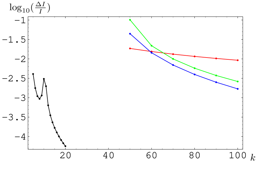
Figure 4: Variation of the relative accuracy $\frac{\Delta I}{I}$ for scanning $\omega-\omega_{\mu}\in[-\frac{2\pi}{t_{r}},\frac{2\pi}{t_{r}}]$ by $k$ points. By far the best accuracy is achieved with the elliptical extrapolation of 4 points around the real axis (black dots). For an approximation by a line between two points (red, largest at large $k$), a second order polynomial $y(x)$ fitted to three points (green, second largest at large $k$), and a third order polynomial $y(x)$ fitted to four pints (blue, third largest at large $k$) all lead to much worth accuracies and/or computation times.

II.3 Comparison of results for polarized modes and coupling

To demonstrate the excellent agreement between these numerical solutions and tracking, we depict Fig. 5 where one HOM with horizontal polarization has been fixed at $f_{x}=2.2$GHz, and another has been varied for $f_{y}\in[1.2,3.2]$GHz. The optics was completely coupled with $T_{12}=T_{34}=0$ and $T_{31}=-T_{14}=10^{-6}\frac{m}{eV/c}$. Several things can be observed: (1) since tracking is relatively time consuming, only relatively few frequencies for the second HOM have been evaluated, but all of them lie exactly on the curve that follows form the dispersion relation. (2) The threshold current varies strongly when the second HOM is varied, but the agreement with tracking shows that this is not numerical noise but a consequence of the coupling between the two polarized modes whose frequencies are very far apart. (3) There are frequencies where the threshold current is relatively small, these are frequencies where $\cos(\omega_{1}t_{b})\approx\cos(\omega_{2}t_{b})$ in agreement with Eq. (36). The displayed minima appear at $(3\cdot 1.3-2.2)$GHz, $2.2$GHz, and $(4\cdot 1.3-2.2)$GHz. But the regions with reduced threshold are relatively wide; in particularly they are much wider than the width of HOM resonances.

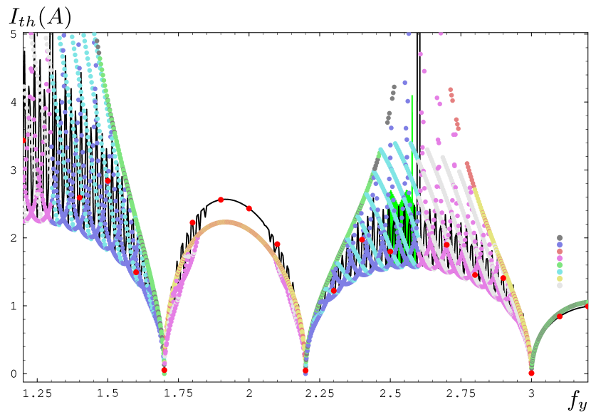
Figure 5: Threshold current for one horizontal HOM with $f_{x}=2.2$GHz as a function of the frequency $f_{y}$ of a vertical HOM. Black curve: dispersion relation, Red dots: tracking, Colored curves: the different applicable approximations derived above.

Depicted in color are the values obtained by approximations derived above. It is apparent that the approximations are not always very good, especially that they lead to values that are too large. A magnification in Fig.6 shows that the reason for that is that the approximate formulas lead to parabolic shapes that have the correct minimum value, but not the correct width. This is important since it shows that the formulas can be used to find the correct minimum value as a conservative estimate. Furthermore, the magnifications again show the good agreement with tracking results.

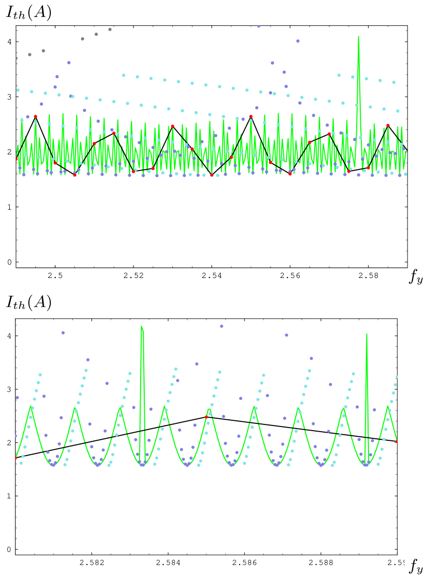
Figure 6: Magnification of regions in Fig. 5

Here an important note is in place. Once place where a strong dip occurs is when $\omega_{1}\approx\omega_{2}$. And this dip is much wider than the width of the HOM resonance of $\omega_{\lambda}/Q\lambda$, showing that the two modes clearly do not decouple when they are separated by more than their width. For nominally circular symmetric cavities, HOMs are not degenerate due to construction errors and each mode splits into two mode with typically a few MeV distance. But the dip is much wider than that, showing that an appropriate advantage of BBU suppression by damping can in general only be realized when polarized cavities are designed, i.e. cavities where the horizontal and vertical dimensions are designed to be slightly different, leading to HOM frequencies that differ by several 10MeV in the two planes.

The question arises how far the HOM frequencies have to be apart. In Fig. 7 we show for the Cornell ERL how $I_{th}$ changes with $\Delta f_{xy}$. In order to avoid averaging over many different frequency distributions we have here chosen the same two HOM frequencies for each of the 320 cavities. The data indicates that a mode separation of $60$MHz is sufficient. This has been used to compute the very large recirculating BBU threshold current of close to 2.5A for this accelerator. It should be noted that only the two dominant HOMs were considered in this simulation and a detailed study is in order when such high currents are sought. The Cornell ERL is designed for 100mA and this calculation indicates that polarized cavities with a coupled optics provide a very comfortable safety margin with respect to this instability.

Figure 7: Dependence of $I_{th}$ on $\Delta f_{xy}$ for the Cornell ERL.

II.4 Approximation for $N$ polarized HOMS in one cavity

As a first approximation one can assume that one component of the eigenvectors in Eq. II will be very large. This would lead to a decoupling of HOMs so that each HOM could be treated separately, as for a single degree of freedom. One could therefore derive the threshold with the smallest current for each individual HOM, and this would approximate the threshold for the complete accelerator. When all these thresholds are very large, one has to investigate the next approximation, where the eigenvector has two dominant components. In this case the eigenvalues are determined from a $2\times 2$ matrix corresponding to Eq. (15). The threshold current has to be computed for each pair of HOMs. The smallest current obtained for one pair of polarized modes then approximates the threshold current of the full accelerator.

III Polarized HOMs in many cavities and for multiple turns

Recirculating linacs with many cavities and several recirculation loops have been considered early on Bisognano87_01 ; Krafft89 . In hoff04 a description for arbitrary recirculation times has been presented. Here we want to extend this description to include orbit coupling and polarized modes. As far as possible we retain the notation of these earlier papers. The $N$ higher order modes, which can be associated with different cavities, are numbered by an index $i$. The $N_{p}$ passes through the linac are numbered by an index $I$. The horizontal and vertical phase space coordinates that the beam has at time $t$ in the HOM $i$ during turn $I$ is denoted $\vec{z}_{i}^{I}(t)=(x_{i}^{I}(t),p_{xi}^{I}(t),y_{i}^{I}(t),p_{yi}^{I}(t))^{T}$. The $4\times 4$ transport matrix that transports the phase space vector $\vec{z}_{j}^{J}$ at HOM $j$ during turn $J$ to $\vec{z}_{i}^{I}$ is denoted ${\bf T}_{ij}^{4I\!J}$ and the time it takes to transport a particle from the beginning of the first turn to HOM $i$ during turn $I$ is denoted $t_{i}^{I}$. The beam is propagated from after HOM $i-1$ to after HOM $i$ by

$$\vec{z}_{i}^{I}(t)={\bf T}_{ii-1}^{4II}\cdot\vec{z}_{i-1}^{I}(t-[t_{i}^{I}-t_{i-1}^{I}])+\frac{e}{c}\vec{V}_{i}(t)\ ,$$ (41)

with $\vec{V}_{i}=V_{i}(0,\cos\theta_{i},0,\sin\theta_{i})^{T}$. This equation can be iterated to obtain the phase space coordinates as a function of the HOM strength that creates the orbit oscillations. With the matrix

$${\bf T}_{ij}^{I\!J}=\left(\begin{array}[]{cc}({\bf T}_{ij}^{4I\!J})_{12}&({\bf T}_{ij}^{4I\!J})_{14}\\ ({\bf T}_{ij}^{4I\!J})_{32}&({\bf T}_{ij}^{4I\!J})_{34}\end{array}\right)$$ (42)

one obtains

$$\vec{x}_{i}^{I}(t) = \sum_{J=1}^{I}\sum_{j=1}^{N_{IJ}(i-1)}{\bf T}_{ij}^{I\!J}\vec{e}_{i}\frac{e}{c}V_{j}(t-[t_{i}^{I}-t_{j}^{J}])\ ,$$ (43)

$$N_{I\!J}(i-1) = \begin{cases}N,&\text{if $I\neq J$;}\\ i-1,&\text{if $I=J$.}\end{cases}$$ (44)

The strength $V_{i}(t)$ of the HOM $i$ with polarization direction $\vec{e}_{j}$ is created by all particles that have traveled through that HOM via the integral

$$V_{i}(t)=\int_{-\infty}^{\infty}\sum_{I=1}^{N_{p}}W_{i}(t-t^{\prime})I_{i}^{I}(t^{\prime})\vec{e}_{i}^{T}\vec{x}_{i}^{I}(t^{\prime})dt^{\prime}\ ,$$ (45)

where $I_{i}^{I}(t)$ is the current at time $t$ that the fraction of the beam has which passes the HOM $i$ on turn $I$. Note that $W(t-t^{\prime})=0$ for $t^{\prime}>t$. Combining this with Eq. (43) leads to the following integral-difference equation:

$$V_{i}(t) = \int_{-\infty}^{\infty}\sum_{I=1}^{N_{p}}W_{i}(t-t^{\prime})I_{i}^{I}(t^{\prime})$$

$$\times \frac{e}{c}\sum_{J=1}^{I}\sum_{j=1}^{N_{I\!J}(i-1)}D_{ij}^{I\!J}V_{j}(t^{\prime}-[t_{i}^{I}-t_{j}^{J}])dt^{\prime}\ ,$$

$$D_{ij}^{I\!J} = \vec{e}_{i}^{T}{\bf T}_{ij}^{I\!J}\vec{e}_{j}\ .$$ (47)

This equation is identical to that obtained for one degree of freedom, only that $({\bf T}_{ij}^{I\!J})_{12}$ is replaced by $D_{ij}^{I\!J}$. The following treatment for obtaining the threshold current is therefore identical to that in hoff04 . For completion it is here presented in simplified form, and recommendations for numerical solutions are given.

Now the approximation of short bunches is used. The current is given at time $t$ by pulses that are equally spaced with the distance $t_{b}$,

$$I_{i}^{I}(t)=\sum_{m=-\infty}^{\infty}I_{0}t_{b}\delta(t-t_{i}^{I}-mt_{b})\ .$$ (48)

This reduces the integral to a sum,

$$V_{i}(t) = \frac{e}{c}I_{0}t_{b}\sum_{m=-\infty}^{\infty}\sum_{I=1}^{N_{p}}W_{i}(t-t_{i}^{I}-mt_{b})$$

$$\times \sum_{J=1}^{I}\sum_{j=1}^{N_{I\!J}(i-1)}D_{ij}^{I\!J}V_{j}(mt_{b}+t_{j}^{J})\ .$$

This leads to

$$\tilde{V}^{\Sigma}_{i,t_{i}^{L}/t_{b}}(\omega) = \frac{e}{c}I_{0}t^{2}_{b}\sum_{n=-\infty}^{\infty}\sum_{m=\infty}^{\infty}\sum_{I=1}^{N_{p}}W_{i}(mt_{b}+t_{i}^{L}-t_{i}^{I})$$

$$\times \sum_{J=1}^{I}\sum_{j=1}^{N_{I\!J}(i-1)}D_{ij}^{I\!J}V_{j}([n-m]t_{b}+t_{j}^{J})e^{i\omega nt_{b}}\ .$$

$$= \frac{e}{c}I_{0}\sum_{I=1}^{N_{p}}\tilde{W}^{\Sigma}_{i,t_{i}^{L}-t_{i}^{I}}\sum_{J=1}^{I}\sum_{j=1}^{N_{I\!J}(i-1)}D_{ij}^{I\!J}\tilde{V}^{\Sigma}_{j,t_{j}^{J}/t_{b}}(\omega)\ .$$

If a vector $\vec{V}$ is introduced that has the coefficients $\tilde{V}^{\Sigma}_{i,t_{i}^{I}}$, this equation can be written in matrix form,

$$\frac{1}{I_{0}}\vec{V}={\bf M}(\omega)\vec{V}\ ,$$ (51)

with the matrix coefficients

$$M_{ij}^{LJ} = \frac{e}{c}t_{b}\sum_{I=J+\Theta_{j,i}}^{N_{p}}\tilde{W}_{i,[t_{i}^{L}-t_{i}^{J}]/t_{b}}(\omega)D_{ij}^{I\!J}$$

$$\Theta_{j,i} = \begin{cases}1,&\text{if $j\geq i$;}\\ 0,&\text{otherwise.}\end{cases}$$ (52)

Note that $\tilde{W}^{\Sigma}_{i,[t_{i}^{L}-t_{i}^{I}]/t_{b}}=\tilde{W}^{\Sigma}_{i,\delta_{i}(I,L)}e^{i\omega Top(\frac{t_{i}^{I}-t_{i}^{L}}{t_{b}})t_{b}}$ where ${\rm Top}(x)$ is the smallest integer that is equal to or larger than $x$ and $\delta_{i}(I,L)={\rm mod}(t_{i}^{I}-t_{i}^{L},t_{b})$. With Kronecker $\hat{\delta}_{ik}$ this determines the matrices ${\bf W}$ and ${\bf U}$ to be

$$W_{ik}^{LI} = \frac{e}{c}t_{b}w_{i}(\delta(I,L))e^{i\omega{\rm Top}(\frac{t^{I}-t^{L}}{t_{b}})t_{b}}\delta_{ik}\ ,$$ (53)

$$U_{kj}^{I\!J} = T_{kj}^{I\!J}\Theta_{I,J+\Theta_{j,k}}\ .$$ (54)

For each frequency $\omega$, $I_{0}^{-1}$ is an eigenvalue of ${\bf M}(\omega)$. Since the eigenvalues are in general complex, but $I_{0}$ has to be real, the threshold current is determined by the largest real eigenvalue of ${\bf M}(\omega)$. The matrix has the properties

$${\bf M}(\omega+\frac{2\pi}{t_{b}})={\bf M}(\omega)\ ,\ \ {\bf M}(-\omega^{*})={\bf M}^{*}(\omega)\ ,$$ (55)

and it is therefore again sufficient to investigate $\omega\in[0,\pi/t_{b}]$ to find the threshold current.

Note that $V_{N}^{N_{p}}$ never appears since the last kick on the last turn does not feed back to any HOM, so that the dimension of ${\bf M}$ can be reduced by one to $N\cdot N_{p}-1$. Furthermore the dimension can be reduced when two fractional parts $\delta_{i}^{I}$ and $\delta_{i}^{J}$ are equal since then $V_{i}^{I}$ and $V_{i}^{J}$ are identical.

III.1 Multi turn operation and cavity misalignments

Since the formalism presented here that includes polarized modes and coupled optics is identical to the formalism in one degree of freedom, only that $({\bf T}_{ij}^{I\!J})_{12}$ has been replaced by $D_{ij}^{I\!J}$, all conclusions about multi turn recirculating and multi turn ERLs hold. For example, in hoff04 it was concluded that for one HOM and for $N_{p}$ passes through the linac, the threshold current should roughly scale as $N_{p}(2N_{p}-1)$. The origin of this conclusion results from the double sum $\sum_{I=1}^{N_{p}}\sum_{J=1}^{I}$. Since the same summation appears, this conclusion holds also for polarized modes with coupling.

For misaligned cavities, HOMs are excited even when the current is smaller than the threshold current. This can lead to large beam excursions, and in hoff04 it was analyzed for what currents these excursions become extremely large. It was found that the BBU threshold current is always smaller than the current for which these orbit excursions would get very large. Since the here presented formalism with coupling and polarized modes has the same formal structure, this conclusion again holds.

III.2 Comments about numerical solutions

As pointed out above where numerical solutions for one return loop and two HOMs were found, it is very essential to systematically search for real values for the eigenvalues of ${\bf M}$. Each eigenvalue traces out curves in the complex plain when $\omega$ is varied in the region $[0,\pi/t_{b})$, however eigenvalue finders usually do not return eigenvalues in any particular order, so that these curves cannot be observed easily. If they could be observed, then ellipses could be fitted to these curves and the intersection of the curve with the real axis could very efficiently be found for each eigenvector.

We therefore recommend a sorting algorithm that sorts eigenvalues rather robustly: (1) Normalize each eigenvector. (2) Sort these vectors according to their largest component, i.e. the vector which has its largest component in position 1 is the first vector, if there are more than one of this kind, the one with the largest coefficient can be chosen as first vector, etc. (3) Associate the eigenvalues in the order of these eigenvectors. Small changes of $\omega$ do not change the relative size of the eigenvector elements much. The intersection of the curve $\lambda_{i}(\omega)$ with the real axis can now be found for each eigenvector. This procedure leads to an enormous speed advantage over simply scanning all eigenvalues for a mesh of $\omega\in[0,\pi/t_{b}]$, and choosing the largest eigenvalue that is reasonably close to the real axis.

References

- (1) M. Tigner, Nuovo Cimento 37, 1228 (1965).
- (2) S.M. Gruner, M. Tigner (eds.), Report No. CHESS 01-003, 2001.
- (3) G.H. Hoffstaetter et al., in Proceedings of the 2003 Particle Accelerator Conference, Portland, OR (IEEE, Piscataway, NJ, 2003), pp. 192-194.
- (4) M.W. Poole et al., in Proceedings of the 2003 Particle Accelerator Conference, Portland, OR (IEEE, Piscataway, NJ, 2003), pp. 189-191.
- (5) S.V. Benson et al., in Proceedings of the 2001 Particle Accelerator Conference, Chicago, IL (IEEE, Piscataway, NJ, 2001), pp. 249-252.
- (6) M. Sawamura et al., in Proceedings of the 2003 Particle Accelerator Conference, Portland, OR (IEEE, Piscataway, NJ, 2003), pp. 3446-3448.
- (7) G.N. Kulipanov, A.N. Skrinsky, N.A. Vinokurov, J. Synchrotron Rad. 5, 176 (1998).
- (8) T. Suwada et al., in Proceedings of the 2002 ICFA Beam Dynamics Workshop on Future Light Sources, Japan.
- (9) L. Merminga et al., in Proceedings of the 2002 European Particle Accelerator Conference, Paris, France, (CERN, Geneva, 2002), pp. 203-205.
- (10) I. Ben-Zvi et al., in Proceedings of the 2003 Particle Accelerator Conference, Portland, OR (IEEE, Piscataway, NJ, 2003), pp. 39-41.
- (11) G.H. Hoffstaetter and I.V. Bazarov, “Beam-breakup instability theory for energy recovery linacs”, Phys. Rev. ST AB 7, 054401 (2004).
- (12) J.J. Bisognano, R.L. Gluckstern, in Proceedings of the 1987 Particle Accelerator Conference, Washington, DC (IEEE Catalog No. 87CH2387-9), pp. 1078-1080.
- (13) G.A. Krafft, J.J. Bisognano, in Proceedings of the 1987 Particle Accelerator Conference, Washington, DC (IEEE Catalog No. 87CH2387-9), pp. 1356-1358.
- (14) R.E. Rand, Recirculating electron accelerators (Harwood Academic Publishers, New York, 1984), Section 9.5.
- (15) N.S.R. Sereno, Ph.D. Dissertation, University of Illinois, 1994
- (16) K. Beard, L. Merminga, B.C. Yunn, in Proceedings of the 2003 Particle Accelerator Conference, Portland, OR (IEEE, Piscataway, NJ, 2003), pp. 332-334.
- (17) L. Merminga, I.E. Campisi, D.R. Douglas, G.A. Krafft, J. Preble, B.C. Yunn, in Proceedings of the 2001 Particle Accelerator Conference, Chicago, IL (IEEE, Piscataway, NJ, 2001), pp. 173-175.
- (18) E. Pozdeyev, ”Regenerative multipass beam breakup in two dimensions”, Phys. Rev. ST AB 8, 054401 (2005).
- (19) R.E. Rand and T.I. Smith, Beam optical control of beam breakup in a recirculating electron accelerator, Particle Accelerators, Vol. 11, pp. 1-13 (1980)
- (20) C.D. Tennant, K.B. Beard, D.R. Kouglas, K.C. Jordan, L.Merminga, E.G. Pozdeyev, “First observations and suppression of multipass, multibunch beam breakup in the Jefferson Laboratory free electron laser upgrade”, Phys. Rev. ST AB 8, 074403 (2005).
- (21) B.C. Yunn, in a contribution to the working group 2 of the ERL workshop (2005)
- (22) G.H. Hoffstaetter, I.V. Bazarov, S. Belomestnykh, D.H. Bilderback, M.G. Billing, J.S-H. Choi, Z. Greenwald, S.M. Gruner, Y. Li, M. Liepe, H. Padamsee, D. Sagan, C.K. Sinclair, K.W. Smolenski, C. Song, R.M. Talman, M. Tigner, “Status of a Plan for an ERL Extension to CESR”, Proceedings PAC05, Knoxville/TN (2005)
- (23) M. Liepe, “Conceptual layout of the cavity string of the Cornell ERL main linac cryomodule”, Proceedings SRF03, Travemünde/FRG (2003)
- (24) G.A. Krafft, J.J. Bisognano, S. Laubach, unpublished, 1987.