Viscous fingering of miscible slices

Abstract

Viscous fingering of a miscible high viscosity slice of fluid displaced by a lower viscosity fluid is studied in porous media by direct numerical simulations of Darcy’s law coupled to the evolution equation for the concentration of a solute controlling the viscosity of miscible solutions. In contrast with fingering between two semi-infinite regions, fingering of finite slices is a transient phenomenon due to the decrease in time of the viscosity ratio across the interface induced by fingering and dispersion processes. We show that fingering contributes transiently to the broadening of the peak in time by increasing its variance. A quantitative analysis of the asymptotic contribution of fingering to this variance is conducted as a function of the four relevant parameters of the problem i.e. the log-mobility ratio $R$, the length of the slice $l$, the Péclet number $Pe$ and the ratio between transverse and axial dispersion coefficients $\varepsilon$. Relevance of the results is discussed in relation with transport of viscous samples in chromatographic columns and propagation of contaminants in porous media.

I Introduction

Viscous fingering is an ubiquitous hydrodynamic instability that occurs as soon as a fluid of given viscosity displaces another more viscous one in a porous medium [1]. As such, the typical example usually presented for this instability is that of oil recovery for which viscous fingering takes place when an aqueous solution displaces more viscous oil in underground reservoirs. This explains why numerous articles devoted to the theoretical and experimental analysis of fingering phenomena have appeared in the petroleum engineering community [1]. For what concerns the geometry, theoretical works typically focus on analyzing the stability properties and nonlinear dynamics of an interface between two semi-infinite domains of different viscosity. In the same spirit, experimental works done either in real porous media or in a model Hele-Shaw system (two parallel plates separated by a thin gap width) consist in injecting continuously a low viscous fluid into the medium initially filled with the more viscous one. The attention is then focused on the dynamics of the interface between the two regions. The instability develops and the fingers grow continuously in time until the displacing fluid has invaded the whole experimental system. As long as the experiment runs (i.e. until the displacing fluid reaches the outlet), the instability develops. Dispersion of one fluid into the other may lead to a slight stabilization in time nevertheless this stabilization is usually negligible on the time scale of the experiment and for high injection rates.

The situation is drastically different in other important applications in which viscous fingering is observed, such as in liquid chromatography or groundwater contamination. Liquid chromatography is used to separate the chemical components of a given sample by passing it through a porous medium. In some cases, and typically in preparative or size exclusion chromatography, the viscosity of the sample is significantly different than that of the displacing fluid (the eluent). Displacement of the sample by the eluent of different viscosity leads then to viscous fingering of either the front or the rear interface of the sample slice, leading to deformation of the initial planar interface. This fingering is dramatic for the performance of the separation technique as it contributes to peak broadening and distortions. Such conclusions have been drawn by several authors that have shown either experimentally [6, 3, 4, 5, 2, 7, 8] or numerically [7, 8] the influence of viscous fingering on peak deformations.

In groundwater contamination and more generally soil contamination, it is not rare that the spill’s extent is finite due to a contamination localized in space and/or time. If the spill’s fluid properties are different than that of water, and in particular, if they have different viscosity and/or density [9, 10], fingering phenomena may influence the spreading characteristics of the contaminated zone. For ecological reasons, it is important then to quantify to what extent fingering will enlarge the broadening in time of this polluted area.

Nonlinear simulations of fingering of finite samples have been performed in the past by Tucker Norton, Fernandez et al. [7, 8] in the context of chromatographic applications, by Christie et al. in relation to “Water-Alternate Gas” (WAG) oil recovery techniques [11] as well as by Zimmerman [12] and have shown the influence of fingering on the deformation of the sample without however investigating the asymptotic dynamics. Manickam and Homsy, in their theoretical analysis of the stability and nonlinear dynamics of viscous fingering of miscible displacements with nonmonotonic viscosity profiles have further stressed the importance of reverse fingering in the deformation of finite extent samples [13, 14]. Their parametric study has focused on analyzing the influence of the endpoint and maximum viscosities on the growth rate of the mixing zone.

In this framework, the objectives of this article are twofold: first, we analyze the nonlinear dynamics of viscous fingering of miscible slices in typical analytical chromatographic and groundwater contamination conditions in order to underline its specificities and, second, we quantify the asymptotic contribution of viscous fingering to the broadening of the output peaks as a function of the important parameters of the problem. From a numerical point of view, the only difference with regard to most of the previous works devoted to viscous fingering [15, 16, 17] is the initial condition which is now a sample of finite extent instead of the traditional interface between two semi-infinite domains. As we show, this has an important consequence: if the longitudinal extent of the slice is small enough with regard to the length of the migration zone, dispersion becomes of crucial importance as it leads to such a dilution of the displaced sample into the bulk fluid before reaching the measurement location that fingering just dies out. As a consequence fingering is then only a transient phenomenon and the output peak of the diluted sample may look Gaussian even if its variance is larger than that of a pure diffusive dynamics because of transient fingering. This explains why the importance of fingering phenomena in chromatography and soil contamination has been largely underestimated or ignored in the literature. We perform here numerical simulations to compute the various moments of the sample distribution as a function of time when fingering takes place. This allows us to extract the contribution of viscous fingering to the variance of the averaged concentration profile and to understand how this contribution varies with the important parameters of the problem which are the log-mobility ratio $R$ between the viscosity of the sample and that of the bulk fluid, the Péclet number $Pe$, the dimensionless longitudinal extent $l$ of the slice and the ratio $\varepsilon$ between the transverse and longitudinal dispersion coefficients. The outline of the article is the following. In Sec. II, we introduce the model equations of the problem. Typical experimental parameters for liquid chromatography and groundwater contamination applications are discussed in Sec. III. The characteristics of the fingering of a miscible slice are outlined in Sec. IV, while a discussion on the moments of transversely averaged profiles is done in Sec. V. Eventually, a parametric study is conducted in Sec. VI before a discussion is made.

II Model system

Our model system is a two-dimensional porous medium of length $L_{x}$ and width $L_{y}$ (Fig. 1). A slice of fluid 2 of length $W$ is injected in the porous medium initially filled with carrier fluid 1. This fluid 2, which is a solution of a given solute of concentration $c_{2}$ in the carrier, will be referred in the following as the sample.

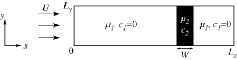
Figure 1: Sketch of the system.

This sample is displaced by the carrier fluid 1 in which the solute concentration $c$ is equal to $c_{1}=0$. Assuming that the viscosity of the medium is a function of the concentration $c$ and that the flow is governed by Darcy’s law, the evolution equations for the system are then:

$$\underline{\nabla}\cdot\underline{u} = 0,$$ (1)

$$\underline{\nabla}p = -\frac{\mu(c)}{K}\underline{u},$$ (2)

$$\frac{\partial c}{\partial t}+\underline{u}\cdot\underline{\nabla}c = D_{x}\frac{\partial^{2}c}{\partial x^{2}}+D_{y}\frac{\partial^{2}c}{\partial y^{2}},$$ (3)

where $\mu$ is the viscosity of the fluid, $K$ is the permeability of the medium, $p$ is the pressure and $\underline{u}=(u,v)$ is the two-dimensional velocity field. The displacing fluid is injected in a uniform manner with a mean velocity $U$ along the $x$ direction. $D_{x},D_{y}$ are the dispersion coefficients along the flow direction and perpendicular to it respectively. The characteristic speed $U$ is used to define a characteristic length $L_{c}=D_{x}/U$ and time $\tau_{c}=D_{x}/U^{2}$. We nondimensionalize space, speed and time by $L_{c},U$ and $\tau_{c}$ respectively. Pressure, viscosity and concentration are scaled by $\mu_{1}D_{x}/K$, $\mu_{1}$ and $c_{2}$, where $\mu_{1}$ is the viscosity of the displacing fluid and $c_{2}$ the initial concentration of the sample. The dimensionless equations of the system become

$$\underline{\nabla}\cdot\underline{u} = 0,$$ (4)

$$\underline{\nabla}p = -\mu(c)\underline{u},$$ (5)

$$\frac{\partial c}{\partial t}+\underline{u}\cdot\underline{\nabla}c = \frac{\partial^{2}c}{\partial x^{2}}+\varepsilon\frac{\partial^{2}c}{\partial y^{2}},$$ (6)

where $\varepsilon=D_{y}/D_{x}$. If $\varepsilon=1$, dispersion is isotropic while $\varepsilon\neq 1$ characterizes anisotropic dispersion. Switching to a coordinate system moving with speed $U$, i.e. making the change of variables $x^{\prime}=x-t,y^{\prime}=y$, $\underline{u}^{\prime}=\underline{u}-\underline{i}_{x}$ with $\underline{i}_{x}$ being the unit vector along $x$, we get, after dropping the primes:

$$\underline{\nabla}\cdot\underline{u} = 0,$$ (7)

$$\underline{\nabla}p = -\mu(c)(\underline{u}+\underline{i}_{x}),$$ (8)

$$\frac{\partial c}{\partial t}+\underline{u}\cdot\underline{\nabla}c = \frac{\partial^{2}c}{\partial x^{2}}+\varepsilon\frac{\partial^{2}c}{\partial y^{2}}.$$ (9)

We suppose here that the viscosity is an exponential function of $c$ such as:

$$\mu(c)=e^{Rc},$$ (10)

where $R$ is the log-mobility ratio defined by $R=ln(\mu_{2}/\mu_{1})$, where $\mu_{2}$ is the viscosity of the sample and, as said before, $\mu_{1}$ is the viscosity of the displacing fluid (Fig. 1). If $R>0$, then we have a low viscosity fluid displacing a high viscosity sample and the rear interface of the sample will be unstable with regard to viscous fingering. If $R<0$, then the sample is the less viscous fluid and the front interface of the slice will then develop fingering. In our simulations, we consider the $R>0$ situation.

Introducing the stream function $\psi$ such that $u=\partial\psi/\partial y$ and $v=-\partial\psi/\partial x$, taking the curl of Eq. (8), we get our final equations [18]:

$$\nabla^{2}\psi=R\left(\frac{\partial\psi}{\partial x}\frac{\partial c}{\partial x}+\frac{\partial\psi}{\partial y}\frac{\partial c}{\partial y}+\frac{\partial c}{\partial y}\right),$$ (11)

$$\frac{\partial c}{\partial t}+\frac{\partial\psi}{\partial y}\frac{\partial c}{\partial x}-\frac{\partial\psi}{\partial x}\frac{\partial c}{\partial y}=\frac{\partial^{2}c}{\partial x^{2}}+\varepsilon\frac{\partial^{2}c}{\partial y^{2}}.$$ (12)

This model is numerically integrated using a pseudo-spectral code introduced by Tan and Homsy [15] and successfully implemented for various numerical studies of fingering [19, 20]. The two-dimensional domain of integration is, in dimensionless units, of size $Pe\times L$ where $Pe=UL_{y}/D_{x}$ is the dimensionless width which is nothing else than the Péclet number of the problem, while $L=UL_{x}/D_{x}$. The dimensionless length of the sample is $l=UW/D_{x}$. The initial condition corresponds to a convectionless fluid ($\psi=0$ everywhere) embedding a rectangular sample of concentration $c=1$ and of size $Pe\times l$ in a $c=0$ background. The middle of the sample is initially located at $x=2L/3$. In practice, for the simulations, the initial condition corresponds to two back to back step functions between $c=0$ and $c=1$ with an intermediate point where $c=\frac{1}{2}+A\cdot r$, $r$ being a random number between 0 and 1 and $A$ the amplitude of the noise (typically of the order of $10^{-3}$). This noise is necessary to trigger the fingering instability on reasonable computing time. If $A=0$, numerical noise will ultimately seed the fingering instability but on a much longer time scale. The boundary conditions are periodic in both directions. This is quite standard along the transversal direction $y$. This does not make any problem along the $x$-axis as $c=0$ at both $x=0$ and $x=L$. The problem is controlled by four dimensionless parameters: the log-mobility ratio $R$, the Péclet number $Pe$, the initial length of the injected sample $l$ and the ratio between transverse and longitudinal dispersion coefficients $\varepsilon$.

III Experimental values of parameters for two applications

In order to perform numerical simulations, let us compute the order of magnitude of the main parameters (Péclet number $Pe$, length of the sample $l$) for both a liquid chromatography experiment and for the propagation of contaminants in a porous medium (groundwater contamination).

III.1 Chromatographic applications

First of all, let us note that in most chromatographic applications, heterogeneous chemistry (particularly adsorption and desorption phenomena) is crucial to the separation process and will undoubtedly affect possible fingering processes. We neglect such physicochemical interactions in this first approach focusing on the effect of viscous fingering on an unretained compound. A typical chromatographic column has a diameter $d=4.6$ mm, a length $L_{x}=150$ mm and consists of a porous medium packed with porous particles, the total (intraparticle and interparticle) porosity being equal to 0.7. The volume of the sample introduced in the column is of the order of 20 $\mu$l, injected at a flow rate $Q\simeq 1$ ml min^-1. The extent of the injected sample is then $W\simeq 1.7\,10^{-3}$ m and the speed of the flow $U\simeq 1.4\,10^{-3}$ m s^-1. The longitudinal and transverse dispersion coefficients are typically $D_{x}=1.43\,10^{-8}$ m² s^-1 [21] and $D_{y}=5.65\,10^{-10}$ m² s^-1 [22]. These parameters allow one to define a characteristic length $L_{c}=D_{x}/U$ and a characteristic time $\tau_{c}=D_{x}/U^{2}$. As a result, the Péclet number $Pe=Ud/D_{x}$ is here nothing else than the dimensionless diameter i.e. $Pe=d/L_{c}\simeq 460$, while the dimensionless longitudinal extent of the sample becomes $l=W/L_{c}\simeq 170$. The dispersion ratio is equal to $\varepsilon=D_{y}/D_{x}\simeq 0.04$. As a typical transit time from inlet to outlet takes roughly $\tau=100$ s, the dimensionless time of a simulation should be of the order of $T=\tau/\tau_{c}\simeq 15000$ to account for a realistic time to characterize the properties of the output peaks.

III.2 Soil contamination

The effects of fluid viscosity and fluid density may be important in controlling groundwater flow and solute transport processes. Recently, a series of column experiments were conducted and analyzed by Wood et al. [10] to provide some insight into these questions. The experiments were performed in fully saturated, homogeneous and isotropic sand columns (porosity equals to 0.34 and $\varepsilon=1$) by injecting a 250 ml pulse of a known concentration solution at a flow rate $Q=0.015$ m³/day. Their experimental setup consists of a vertical pipe $L_{x}=0.91$ m in length with a diameter of $d=0.15$ m. Assuming the medium to be homogeneous and the dispersion coefficient $D$ as isotropic, a typical value for the aquifer dispersion coefficient is $D=0.1$ m²/month i.e. $D\simeq 3.86\,10^{-8}$ m² s^-1 [23]. In the same spirit as above, we compute the Péclet number to be of the order of $Pe\simeq 110$, while the dimensionless length of the sample is $l\simeq 30$.

Based on these two examples, let us now investigate the properties of fingering of finite slices for typical values of parameters in the range computed above i.e. $Pe\sim 100-500$, $\varepsilon\sim 0.04-1$, $l\sim 0-500$, while $R$ is supposed to be of order one.

IV Fingering of a finite width sample

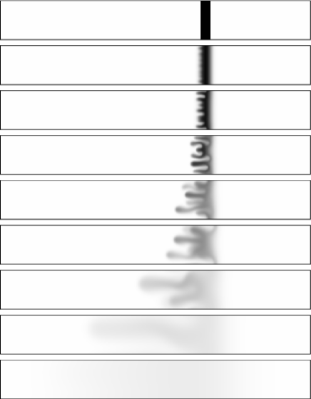
Figure 2: Density plots of concentration at successive times in the frame moving at the velocity $U$. From top to bottom: $t$=0, 500, 700, 1000, 1500, 2000, 5000, 15000 and 60000 ($Pe=512$, $l=128$, $R=2$, $\varepsilon=1$).

Figure 2 shows in a frame moving with the injection velocity $U$ the typical viscous fingering of the rear interface of a sample displaced from left to right by a less viscous fluid. The system is shown at successive times using density plots of concentration with black (resp. white) corresponding to $c=1$ (resp. $c=0$). While the front interface is stable, the back interface develops fingers such that the center of gravity of the sample is displaced in the course of time towards the back with regard to its initial position. This dynamics results from the fact that the stable zone acts as a barrier to finger propagation in the flow direction leading therefore to reverse fingering. Such a reverse fingering has been well characterized by Manickam and Homsy in their numerical analysis of fingering of nonmonotonic viscosity profiles [14]. After a while, dispersion comes into play and dilutes the more viscous fluid into the bulk of the displacing fluid. As the sample becomes more and more diluted, the effective viscosity ratio decreases in time weakening the source of the instability. Ultimately, dispersion becomes dominant and the sample goes on diluting in the bulk without witnessing any further fingering phenomenon. These successive steps can clearly be observed on the transverse averaged profiles of concentration defined as

$$\bar{c}(x,t)=\frac{1}{Pe}\int_{0}^{Pe}c(x,y,t)dy.$$ (13)

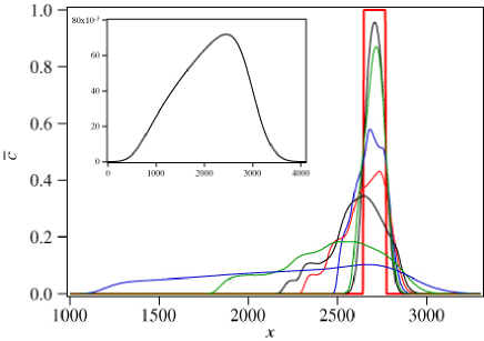
Figure 3: Transverse average profiles of concentration at successive times $t$=0, 500, 700, 1000, 1500, 2000, 5000 and 15000. Insert: transverse average profile of concentration at $t=60000$ ($Pe=512$, $l=128$, $R=2$, $\varepsilon=1$).

As seen on Fig. 3, we first start with two back to back step functions defining an initial sample of extent $l$. During the first stages of the injection, there is a first diffusive regime quickly followed by the fingering of the rear interface corresponding here to the left front. While the right (i.e. frontal) interface features the standard error function characteristic of simple dispersion, the left one shows bumps signaling the presence of fingering. Because the extent of the sample is finite, dispersion and fingering contribute to the fact that the maximum concentration becomes smaller than one, effectively leading to a viscosity ratio between the sample and the bulk that decreases in time. As a consequence, fingering dies out and the transverse profile starts to follow a distorted Gaussian shape. If one waits long enough, the asymmetry of the bell shape diminishes which explains that output peaks in chromatographic columns may look Gaussian even if fingering has occurred during the first stages of the travel of the sample in the column. As computed in the preceding section, a typical dimensionless time of transit in a real chromatographic setup corresponds to 15000 units of time. Figures 2 and 3 show that, after 15000 units of time, fingering is disappearing for this specific set of typical values of parameters, and that dispersion becomes again the dominant mode. As chromatographic columns are generally opaque porous media, it is therefore not astonishing that the presence of viscous fingering has long been totally ignored until recent experimental works which have visualized fingering by magnetic resonance or optical imaging [6, 3, 4, 5, 2, 7, 8]. Similarly, tracing of the spatial extent of a contaminant plume at a distance far from the pollution site may lead to measurements of Gaussian-type spreading even if fingering has occurred at early times. The only influence of such fingering appears in the larger variance of the sample than in the case of pure dispersion as we show it next.

V Moments of the transverse averaged profile

The averaged profiles of concentration $\overline{c}(x,t)$ allow to compute the three first moments of the distribution: the first moment $m$

$$m(t)=\frac{\int_{0}^{L}\bar{c}(x,t)xdx}{\int_{0}^{L}\bar{c}(x,t)dx}$$ (14)

is the position of the center of mass of the distribution as a function of time. The second moment is the variance $\sigma^{2}$

$$\sigma^{2}(t)=\frac{\int_{0}^{L}\bar{c}(x,t)[x-m(t)]^{2}dx}{\int_{0}^{L}\bar{c}(x,t)dx}$$ (15)

giving information on the width of the distribution. Eventually, we compute also the third moment, i.e. the skewness

$$a(t)=\frac{\int_{0}^{L}\bar{c}(x,t)[x-m(t)]^{3}dx}{\int_{0}^{L}\bar{c}(x,t)dx}$$ (16)

that gives information concerning the asymmetry of the peak with regard to its mean position.

The variance $\sigma^{2}$ is the sum of three contributions:

$$\sigma^{2}(t)=\sigma^{2}_{i}+\sigma^{2}_{d}+\sigma^{2}_{f},$$ (17)

where $\sigma^{2}_{i}=l^{2}/12$ is the variance due to the initial length of the sample, $\sigma^{2}_{d}=2t$ is the contribution of dispersion in dimensionless units and $\sigma^{2}_{f}$ is the contribution due to the fingering phenomenon. If $R=0$, the displacing fluid and the sample have the same viscosity and no fingering takes place. Hence, in that case, $\sigma^{2}=\sigma^{2}_{i}+\sigma^{2}_{d}=l^{2}/12+2t$. We have checked that this result is recovered by numerical simulations for $R=0$. The integrals in the computation of the moments (14)–(16) are evaluated numerically by using Simpson’s rule. The numerical result is very good if the spatial discretization step $dx$ is small. Typically, we get the exact result for $dx=1$. Unfortunately, $dx=1$ is a resolution too high for fingering simulations especially if one wants to look at the dynamics at very long times. As an example, previous simulations on viscous fingering phenomena [15, 19] were done with larger $dx$ as typical dimensionless fingering wavelengths are around 100 for $R=3$ for instance. Using typically $dx=4$ gives roughly 25 points per wavelength which is numerically reasonable. For what concerns the variance, simulations with $R=0$ and $dx=4$ give the correct $\sigma^{2}_{i}$ at $t=0$ but a constant shift appears so that $\sigma^{2}(t)-l^{2}/12-2t=C$, with $C$ being a constant of the order of $0.1\%$ of $l^{2}/12$. As we are mostly interested in the rate of variation of $\sigma_{f}$, where $\sigma_{f}$ is defined as

$$\sigma_{f}(t)=\sqrt{\sigma^{2}_{f}(t)}=\sqrt{\sigma^{2}(t)-\sigma^{2}_{i}-\sigma^{2}_{d}},$$ (18)

all simulations are done here with $dx=4$. The slight $C$ shift does not affect the value of $\sigma_{f}$ as we have checked it for decreasing values of $dx$.

Figure 4: First three moments of the distribution: (a) Mean position $m$ of the center of mass, (b) Variance $\sigma^{2}$, (c) Skewness $a$ ($Pe=512$, $l=128$, $R=2$, $\varepsilon=1$).

Figure 4 shows the temporal evolution of the first three moments i.e. the deviation $m(t)-m(t=0)$ of the center of mass in comparison to its initial location at $t=0$, the total variance $\sigma^{2}(t)$ and the skewness $a(t)$ for the typical example of Figs. 2 and 3. As fingering occurs quicker than dispersion, the center of gravity of the sample $m(t)$ is displaced towards the back (smaller $x$ values) because of reverse fingering of the rear interface of the sample [Fig. 4(a)]. Fingering contributes to the widening of the peak and thus $\sigma^{2}(t)$ increases [Fig. 4(b)] while the skewness $a(t)$ becomes non zero due to the asymmetry of the fingering instability with regard to the middle of the sample [Fig. 4(c)]. After a while, fingering dies out and the first moment $m(t)$ saturates to a constant indicating that dispersion becomes again the only important dynamical transport mechanism. Note that the skewness $a$ is observed to revert back towards 0 at very long times.

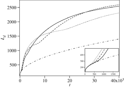
Figure 5: Mixing zone $L_{d}$ as a function of time realized with the same parameters ($Pe=512$, $l=128$, $R=2$, $\varepsilon=1$) and three different values of the amplitude $A$ of the noise seeding the initial condition: ($\cdots$) $A=0.1$, (- -) $A=0.01$, (—) $A=0.001$; (– $\cdot$ –) theoretical curve of a pure diffusive behavior $L_{d}\propto\sqrt{t}$. Insert: zoom on the first stages on the injection. The onset time $t^{*}$, corresponding to the time at which the mixing zone departs from the pure diffusive initial transient, is a decreasing function of $A$.

Onset of fingering is also witnessed in the growth of the mixing zone $L_{d}$ defined here as the interval in which $\bar{c}(x,t)>0.01$ (Fig. 5). An important thing to note is that, after a diffusive transient, fingering appears on a characteristic time scale $t^{*}$, defined as the time for which the mixing zone temporal dependence departs from the pure diffusive regime.

As has already been discussed before [16, 20], the characteristics of the fingering onset time $t^{*}$ and of the details of the nonlinear fingering regime are dependent on the noise amplitude $A$. The higher the noise intensity $A$, the quicker the onset of the instability (Insert in Fig. 5). To get insight into the influence of the relevant physical parameters of the problem, it is therefore necessary to fix the amplitude of the noise to an arbitrary constant as this is not a variable that is straightforwardly experimentally available. In that respect, our results have here typically been obtained for a noise of fixed $A=0.001$. The number of fingers appearing at early times is related to the most unstable wavenumber of the band of unstable modes, nevertheless the location and subsequent nonlinear interaction of the fingers depend on the specific realization of the random numbers series. As a consequence, it is necessary to compute a set of realizations to get statistical information on $\sigma_{f}$, the main quantity of interest here.

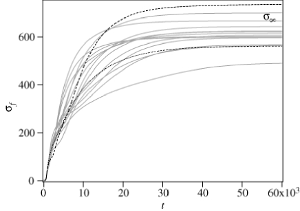
Figure 6: $\sigma_{f}$ as a function of time for 15 numerical simulations realized with the same values of parameters ($Pe=512$, $l=128$, $R=2$, $\varepsilon=1$) but different noise $r$ realizations of identical amplitude $A=10^{-3}$. The dotted and dashed curves correspond to the simulations of Figs. 2 and 7 respectively.

Figure 6 shows the temporal evolution of $\sigma_{f}$ for 15 different noise realizations of identical amplitude for fixed values of the parameters $R,Pe,l$ and $\varepsilon$. As can be seen, if fingering starts always at the same onset time $t^{*}$ for fixed $A$, the contribution to the variance due to fingering saturates to different asymptotic values $\sigma_{\infty}$. This corresponds to slightly different nonlinear interactions of the fingers as can be seen on Figs. 2 and 7 which show the temporal evolution of the fingers for the respectively dotted and dashed curves of Fig. 6. If the patterns observed are very similar during the initial linear phase of viscous fingering, the evolution of the fingers is slightly different in the nonlinear regime, leading to different values of $\sigma_{\infty}$. In particular, merging is observed in Fig. 7 leading to the fast development of one finger and, then, spreading of the stripe of viscous fluid leading to a larger value of $\sigma_{\infty}$.

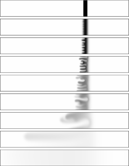
Figure 7: Density plots of concentration for the same values of parameters and same times as in Fig. 2, but a different noise $r$ in the initial condition.

As a consequence, to understand the influence of fingering on the broadening of finite slices, it is necessary to study the parametric dependence of $<\sigma_{\infty}>$, the statistical ensemble averaged asymptotic value of the fingering contribution to the variance.

VI Parameter study

The quantity $<\sigma_{\infty}>$ gives information on the influence of viscous fingering on the broadening of finite samples. In applications such as chromatography and dispersion of contaminants in aquifers, such a broadening is undesirable and it is therefore important to understand the optimal values of parameters for which $<\sigma_{\infty}>$ is minimum given some constraints. In that respect, let us first consider a porous medium in which dispersion is isotropic ($\varepsilon=1$) and let us analyze the subsequent influences of $l$, $R$ and $Pe$. The anisotropic case ($\varepsilon\neq 1$) will eventually be tackled. The mean value $<\sigma_{\infty}>$ is plotted for various values of the parameters, the bar around this mean value spanning the range of asymptotic data between the minimum and maximum observed.

VI.1 Influence of the sample length $l$

The sample length $l$ has been measured to have practically no influence on the onset time $t^{*}$ of the instability. Although Nayfeh has shown that the stability of finite samples could be affected if the two interfaces are close enough [24], we note that, for the smallest value of sample length $l$ considered here ($l=32$), the rear interface features the same initial pattern as the one appearing on the interface between two semi-infinite regions of different viscosities for a same random sequence in the seeding noise. Our samples are thus here long enough for the onset time $t^{*}$ to depend only on the amplitude $A$ of the noise seeding the initial condition and not feel the finite extent of the sample. The length $l$ influences nevertheless the broadening of the peak and thus $<\sigma_{\infty}>$ in particular for small $l$. The points reported in Fig. 8 for two different $Pe$ are obtained for one realization and a same seeding noise $r$ in the initial condition, leading to a typical value of $\sigma_{\infty}$. The smaller the extent $l$ of the sample, the sooner the dilution of the more viscous solution into the bulk of the eluent and thus the less effective fingering. Above a given extent $l_{c}$, $\sigma_{\infty}$ is found to saturate. At first sight, this might appear counterintuitive as one could expect that, for longer samples, fingering is maintained for a longer time thereby enhancing the fingering contribution to the variance. A closer inspection to the finger dynamics shows on the contrary that, after a transient where several fingers appear and interact, only one single finger remains (see Figs. 2 and 7). In the absence of tip splitting, the stretching of the mixing zone becomes then exclusively diffusive as already discussed previously by Zimmerman and Homsy [16, 17]. This is clearly seen in Fig. 5 which shows that the mixing length grows as $\sqrt{t}$ at long times after a linear transient due to fingering. Once the asymptotic diffusive regime is reached, the contribution of fingering to the broadening of the peak dies out and $\sigma_{f}$ saturates to $\sigma_{\infty}$. Above a given critical length $l_{c}$ of the sample, the same asymptotic single finger growing diffusively is reached before the left and right interfaces interact. Hence the same value $\sigma_{\infty}$ is obtained for any $l>l_{c}$. Let us note that the switch from the fingering to the diffusive dynamics appears later in time when $Pe$ is increased. Indeed larger $Pe$ means more fingers that can interact for a longer time before the diffusive regime becomes dominant. As a consequence, $l_{c}$ is an increasing function of $Pe$ as can be seen on Fig. 8. Further studies need to be done to understand the role of $\varepsilon$ and of possible tip splitting occurring for large $Pe$ on the existence and value of the critical length $l_{c}$.

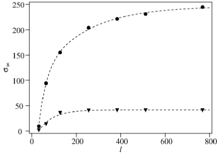
Figure 8: Influence of the sample length $l$ on $\sigma_{\infty}$ for ($\blacktriangledown$) $Pe=64$ and ($\bullet$) $Pe=128$ ($R=2$, $\varepsilon=1$).

The fact that the contribution of fingering to the broadening of the peak saturates beyond a critical length of the sample has important practical consequences for chromatography: if fingering is unavoidable, one might as well load samples of long extent as the contribution of fingering is saturating beyond a given $l_{c}$. For long samples, the efficiency of the process depends then on the competition between $\sigma^{2}_{\infty}$ and $l^{2}/12$, the respective fingering and initial length contributions to the peak’s variance. We can thus predict that for $l_{c}<l<\sigma_{\infty}/\sqrt{12}$, the contribution of fingering is constant and dominates the broadening while for $l>\sigma_{\infty}/\sqrt{12}$, the initial sample length becomes the key factor.

VI.2 Influence of the log-mobility ratio $R$

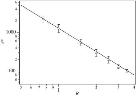
Figure 9: Onset time $t^{*}$ of the instability for increasing values of $R$ ($Pe=256$, $l=128$, $\varepsilon=1$). (—) Best fit of the experimental points: $t^{*}\propto R^{-2}$.

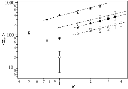
Figure 10: Influence of the log-mobility ratio $R$ on $<\sigma_{\infty}>$ for ($\circ$) $Pe=128,l=128$, ($\bullet$) $Pe=128,l=512$, ($\triangle$) $Pe=256,l=128$, ($\blacktriangle$) $Pe=256,l=512$ ($\varepsilon=1$).

It is easy to foreseen that the larger $R$, the more important the viscous fingering effect [8]. First of all, linear stability analysis of viscous fingering at the interface between two semi-infinite domains [18] predicts that the characteristic growth time of the instability decreases as $R^{-2}$. Although already influenced by the nonlinearities and dependent on the amplitude of the noise, the onset time $t^{*}$ measured in our simulations shows the same trend (Fig. 9). Note that, for very small values of $R$, the onset time becomes very large which explains why, for samples of low viscosity, fingering might not be observed during the transit time across small chromatographic columns or on small scale contamination zone. When $R$ is increased, the viscous fingering contribution to peak broadening $<\sigma_{\infty}>$ is more important (Fig. 10) with a linear dependence suggesting a power law increase for larger $R$.

VI.3 Influence of the Péclet number $Pe$

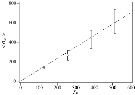
Figure 11: Influence of the Péclet number $Pe$ on $<\sigma_{\infty}>$ ($l=128$, $R=2$, $\varepsilon=1$).

The Péclet number $Pe$ is typically experimentally increased for a given geometry by increasing the injection flow rate $U$. As can be seen on Fig. 11, $<\sigma_{\infty}>$ is found to increase linearly with $Pe$. Fingering induced broadening can thus be minimized by small carrier velocity $U$ as expected. However, the exact influence of the carrier velocity $U$ is difficult to trace because practically, a change in $U$ also modifies the dispersion coefficients and hence the value of $\varepsilon$. In our dimensionless variables, $U$ also enters into the characteristic time and length corresponding respectively to $D_{x}/U^{2}$ and $D_{x}/U$. The concrete influence of the carrier velocity is thus more complicated to trace in reality. For a fixed injection speed, the Péclet number can also be varied by changing the width $L_{y}$ of the system. The linear dependence of $<\sigma_{\infty}>$ on $Pe$ is then related to the fact that in a wider domain, more fingers can remain in competition for a longer time so that a more active fingering is maintained. This also implies that $l_{c}$ is an increasing function of $Pe$. In chromatographic applications, increasing the diameter of the column (i.e. increasing $L_{y}$ here in our model) is thus expected to dramatically increase the influence of fingering in broadening. This explains why fingering really becomes an issue for wide contamination zones and in preparative chromatography where columns of very large diameter (up to one meter) are sometimes constructed.

VI.4 Influence of the ratio of dispersion coefficients $\varepsilon$

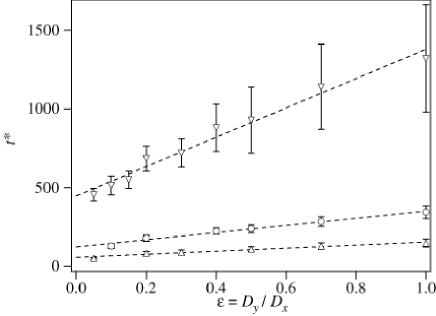
Figure 12: Onset time $t^{*}$ of the instability for increasing values of $\varepsilon$ for different values of the log-mobility ratio: ($\triangledown$) $R=1$, ($\circ$) $R=2$, ($\vartriangle$) $R=3$ ($Pe=128$, $l=128$).

Figure 12 shows the influence of the ratio of dispersion coefficients $\varepsilon=D_{y}/D_{x}$ on the onset time of the instability. As expected from linear stability analysis [18], decreasing $\varepsilon$ has a destabilizing effect as fingering appears then quicker. This is due to the fact that small transverse dispersion inhibits the mixing of the solutions and favors longitudinal growth of the fingers allowing them to survive for a longer time. As a consequence, the less viscous solution instead of being transversely homogeneous invades the more viscous fluid preferably in the longitudinal direction leading to larger mixing zones and hence larger $<\sigma_{\infty}>$. Figure 13 illustrates that decreasing $\varepsilon$ has a dramatic effect on the broadening of the peak. The insert shows the same graphics in logarithmic scale for $\varepsilon$. $<\sigma_{\infty}>$ seems to vary as $\ln(\varepsilon)$ at least for small values of $\varepsilon$. Peak broadening due to fingering is therefore expected to be particularly dramatic for chromatographic applications where $\varepsilon\sim 0.04$.

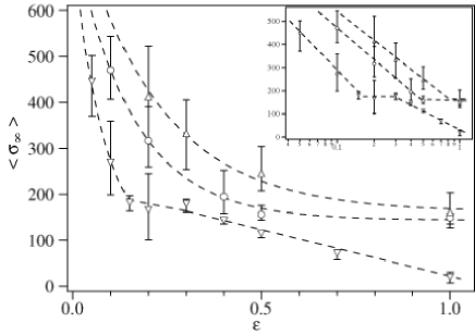
Figure 13: Influence of the ratio between transverse and longitudinal dispersion $\varepsilon$ on $<\sigma_{\infty}>$ for ($\triangledown$) $R=1$, ($\circ$) $R=2$, ($\triangle$) $R=3$ ($Pe=128$, $l=128$). Insert: same data on logarithmic scale for $\varepsilon$.

VII Conclusion

Viscous fingering leads to a mixing between miscible fluids of different viscosity. In the case of viscous slices of finite extent, fingering is a transient phenomenon because the mixing of the two fluids leads to an effective decrease of the log-mobility ratio in time. Transient fingering can nevertheless play an important role because it contributes to distortion and broadening of the sample. In particular, we have shown that, even if the spreading of the sample may look Gaussian at long times because dispersion has again become the leading transport phenomenon, the variance of the peak is larger than expected because of fingering at early times. We have demonstrated this influence by numerical simulations of viscous fingering of miscible finite slices characterizing the onset time of the instability $t^{*}$ and the contribution of fingering to the sample’s variance. It is important to note that quantitative comparison with experimental data is difficult because the exact amplitude of the fingering contribution to the temporal variation of the peak’s variance depends both on the amplitude and spatial realization of the noise seeding the initial condition which varies from one experiment to the other. In this respect, we have computed the ensemble averaged asymptotic fingering contribution to the peak broadening as a function of the four relevant parameters of the problem i.e. the initial length of the sample $l$, the initial log-mobility ratio $R$, the Péclet number $Pe$ and the ratio between transverse and longitudinal dispersion coefficients $\varepsilon$. The broadening of the peaks due to fingering is most important for large $R$ and $Pe$ but small $\varepsilon$ while it saturates above a given initial length $l$ of the sample. In chromatographic columns for which $\varepsilon\sim 0.04$, fingering is thus of crucial importance particularly in preparative chromatography for which the large diameter of the columns lead to large $Pe$ and the high concentration of the samples usually implies large $R$. Similarly, for soil contamination, fingering will be a major problem in the case of stratified media such that $\varepsilon<1$. More work is now needed to explore the generalization of this first approach to the case where both viscosity and density variations as well as heterogeneous chemistry may interplay as is usually the case in the applications analyzed here.

VIII Acknowledgements

We thank G.M. Homsy, P. Colinet, A. Vedernikov and B. Scheid for fruitful discussions. Y. Bertho benefits from a postdoctoral fellowship of the Université Libre de Bruxelles sponsored by the Francqui Foundation which is gratefully acknowledged. A. De Wit thanks also FRFC (Belgium) and the “Communauté française de Belgique - Actions de Recherches Concertées” programme for financial support.

References

- [1] G.M. Homsy, Viscous fingering in porous media, Ann. Rev. Fluid Mech. 19, 271 (1987).
- [2] B.S. Broyles, R.A. Shalliker, D.E. Cherrak and G. Guiochon, Visualization of viscous fingering in chromatographic columns, J. Chromatogr. 822, 173 (1998).
- [3] L.D. Plante, P.M. Romano and E.J. Fernandez, Viscous fingering visualized via magnetic resonance imaging, Chem.Eng. Sci. 49, 229 (1994).
- [4] E.J. Fernandez, C.A. Grotegut, G.W. Braun, K.J. Kirschner, J.R. Staudaher, M.L. Dickson, and V.L. Fernandez, The effects of permeability heterogeneity on miscible viscous fingering: A three-dimensional magnetic resonance imaging analysis, Phys. Fluids 7, 468 (1995).
- [5] D. Cherrak, E. Guernet, P. Cardot, C. Herrenknecht and M. Czok, Viscous fingering: a systematic study of viscosity effects in methanol-isopropanol systems, Chromatographia 46, 647 (1997).
- [6] M. Czok, A. Katti and G. Guiochon, Effect of sample viscosity in high-performance size-exclusion chromatography and its control, J. Chromatogr. 550, 705 (1991).
- [7] E.J. Fernandez, T. Tucker Norton, W.C. Jung and J.G. Tsavalas, A column design for reducing viscous fingering in size exclusion chromatography, Biotechnol. Prog. 12, 480 (1996).
- [8] T. Tucker Norton and E.J. Fernandez, Viscous fingering in size exclusion chromatography: insights from numerical simulation, Ind. Eng. Chem. Res. 35, 2460 (1996).
- [9] C.Y. Jiao and H. Hotzl, An experimental study of miscible displacements in porous media with variation of fluid density and viscosity, Trans. Porous Media 54, 125 (2004).
- [10] M. Wood, C.T. Simmons and J.L. Hutson, A breakthrough curve analysis of unstable density-driven flow and transport in homogeneous porous media, Water Resour. Res. 40, W03505 (2004).
- [11] M.A. Christie, A.H. Muggeridge and J.J. Barley, 3D simulation of viscous fingering and WAG schemes, SPE 21238, presented at the 11th Symposium on Reservoir Simulation, Anaheim, California, February 17-20, 1991.
- [12] W.B.J. Zimmerman, Process Modelling and Simulation with Finite Element Methods (World Scientific, Singapore, 2004).
- [13] O. Manickam and G.M. Homsy, Stability of miscible displacements in porous media with nonmonotonic viscosity profiles, Phys. Fluids A 5, 1357 (1993).
- [14] O. Manickam and G.M. Homsy, Simulation of viscous fingering in miscible displacements with nonmonotonic viscosity profiles, Phys. Fluids 6, 95 (1994).
- [15] C.T. Tan and G.M. Homsy, Simulation of nonlinear viscous fingering in miscible displacement, Phys. Fluids 31, 1330 (1988).
- [16] W.B. Zimmerman and G.M. Homsy, Nonlinear viscous fingering in miscible displacement with anisotropic dispersion, Phys. Fluids A 3, 1859 (1991).
- [17] W.B. Zimmerman and G.M. Homsy, Viscous fingering in miscible displacements : unification of effects of viscosity contrast, anisotropic dispersion, and velocity dependence of dispersion on nonlinear finger propagation, Phys. Fluids A 4, 2348 (1992).
- [18] C.T. Tan and G.M. Homsy, Stability of miscible displacements in porous media: rectilinear flow, Phys. Fluids 29, 3549 (1986).
- [19] A. De Wit and G.M. Homsy, Nonlinear interactions of chemical reactions and viscous fingering in porous media, Phys. Fluids 11, 949 (1999).
- [20] A. De Wit, Miscible density fingering of chemical fronts in porous media: nonlinear simulations, Phys. Fluids 16, 163 (2004).
- [21] J.H. Knox, Band dispersion in chromatography - a new view of A-term dispersion, J. Chromatogr. A 831, 3 (1999).
- [22] J.H. Knox, G.R. Laid and P.A. Raven, Interaction of radial and axial dispersion in liquid chromatography in relation to the ”infinite diameter effect”, J. Chromatogr. 122, 129 (1976).
- [23] S.E. Serrano, Propagation of nonlinear reactive contaminants in porous media, Water Resour. Res. 39, 1228 (2003).
- [24] A.H. Nayfeh, Stability of liquid interfaces in porous media, Phys. Fluids 15, 1751 (1972).