$N$-Electron Giant Dipole States in Crossed Electric and Magnetic Fields

Abstract

Multi-electron giant dipole resonances of atoms in crossed electric and magnetic fields are investigated. Stationary configurations corresponding to a highly symmetric arrangement of the electrons on a decentered circle are derived, and a normal-mode and stability analysis are performed. A classification of the various modes, which are dominated by the magnetic field or the Coulomb interactions, is provided. Based on the mctdh approach, we carry out a six-dimensional wave-packet dynamical study for the two-electron resonances, yielding in particular lifetimes of more than $0.1\mu$s for strong electric fields.

I introduction

Interactions of atoms with strong electric and magnetic fields, in particular crossed fields, have long been the focal point of various research efforts burkova76; rau86; melezhik93; raithel95; zhang95; floethmann96; haggerty97. The conflicting symmetries inherent in the electronic motion in atomic and external fields make for a rich variety of phenomena. In this light they are not only interesting from a theoretical standpoint, such as the hydrogen atom, which constitutes a paradigm for a chaotic system Friedrich97; Herold81:751; Friedrich89:37; Schmelcher98; Gallagher94: Their study also had a major impact on a number of other fields, ranging from semiconductor physics to astrophysics.

However, for a long time theoretical investigations did not go beyond the stage of treating the nucleus as ‘frozen’, the so-called infinite-mass approximation. The model underlying this picture is the concept that the atomic motion could be separated into that of the center of mass and the one relative to it. While this is perfectly justified for translationally invariant systems—going along with the conservation of the total momentum—it ceases to be true in the presence of magnetic fields. Nonetheless, a weaker version of this procedure can be established in the case of (neutral) atoms in homogeneous fields Lamb59; Avr78:431; Herold81:751; Hirsch83. In this pseudo-separation, a conserved quantity termed pseudo-momentum—the total momentum plus a field-dependent compensation—allows to obtain a Hamiltonian that depends on the relative coordinates only. However, that relative motion strongly depends on the center of mass via the pseudo-momentum. This coupling gives rise to some new and interesting effects, such as chaotic diffusion of the center of mass Schm92:305; Schm92:2697, or dynamical self-ionization Schm95:662; melezhik00 for the case of ions.

Yet one of the most prominent among these finite-mass effects is the existence of giant dipole states, where the electrons can be decentered from the nucleus by many $10,000$ atomic units Baye92; Dzyaloshinskii92. The systematic base for this was the gauge-independent generalized potential first derived for hydrogen by Dippel et al. Dip94:4415 and extended to arbitrary atoms by Schmelcher Schm01. It has been applied extensively to study giant dipole states in the two-body case; e.g., hydrogen Dip94:4415 and positronium Ack98:1129; Ack97, where the large inter-particle distance prevents annihilation for up to several years. By contrast, the extension to the multi-electron case has attracted only limited attention. There have been indications for two-electron quasistable giant-dipole states based on a local semiclassical analysis Schm01. The aim of this paper is to both provide a local analysis of general $N$-electron system and investigate the stability of the full quantum-mechanical system. In order to first analyze the $N$-electrons case analytically, we look for stationary points of the so-called generalized potential of the effective relative motion (the ‘giant-dipole configuration’) so as to carry out a normal-mode analysis about these points. Equipped with this insight into the local behavior, we study the exact system $N=2$ numerically using wave-packet propagation. Here we resort to the mctdh method (Multi-Configuration Time-Dependent Hartree) mey03:251; mey98:3011; bec00:1.

This article is organized as follows. In Sec. II, the theoretical framework of the pseudo-separation is reviewed and applied to derive the generalized potential of the relative motion. Sec. III then deals with the stationary points of the generalized potential as a base for the analysis of giant dipole resonances. In the subsequent section, the normal-mode analysis for $N$ electrons is carried out. To this end, the local equations of motion are derived (IV.1), whose eigenmodes and -vectors are computed numerically (IV.2) as the solutions of a quadratic eigenvalue problem. Sec. V contains a wave-packet dynamical study of the two-electron system based on the mctdh method. Results on the stability, spectral properties and lower bounds for the lifetimes of the resonances are presented.

II The $N$-electron atom in crossed electric and magnetic fields

The Hamiltonian of an atom, consisting of $N$ electrons (of mass $m$) and a nucleus (mass $M_{0}$) interacting via the Coulomb potential $V$, reads in the laboratory frame:

$$H=\frac{1}{2m}\sum_{i=1}^{N}\left(\mathbf{p}_{i}-e\mathbf{A}(\mathbf{r}_{i}^{\prime})\right)^{2}+\frac{1}{2M_{0}}\left(\mathbf{p}_{0}+Ze\mathbf{A}(\mathbf{r}_{0}^{\prime})\right)^{2}-e\sum_{i=1}^{N}\mathbf{E}\cdot\mathbf{r}_{i}^{\prime}+Ze\mathbf{E}\cdot\mathbf{r}_{0}^{\prime}+V.$$

Here an electron (index $i\leq N$) has the electric charge $e=-|e|$; the atomic number $Z$ equals the number of electrons $N$ in the neutral case treated here. We consider static electric and magnetic fields, which are accounted for by the electro-static potential $\phi(\mathbf{r})=-\mathbf{E}\cdot\mathbf{r}$ and the vector potential $\mathbf{A}(\mathbf{r})$, whose gauge is not fixed here.

In the field-free case, the translation invariance of the system—going along with the conservation of the total momentum—guarantees a complete separation of the center-of-mass and the relative motion. The vector potential now breaks that symmetry. For the special case of homogeneous fields, though, it was shown that a so-called pseudo-separation of the center-of-mass motion is possible . The key is that even though the total momentum is not conserved, the total pseudo-momentum $\mathbf{K}:=\sum_{a=0}^{N}\mathbf{k}_{a}$ defined in terms of the one-particle pseudo-momenta

$$\mathbf{k}_{i}:=m\mathbf{v}_{i}-e\mathbf{r}_{i}^{\prime}\times\mathbf{B}$$

—and likewise for the nucleus—is constant by construction Avr78:431; Hirsch83; Herold81:751. It can be thought of as the kinetic center-of-mass (CM) momentum plus a magnetic-field-dependent compensation, which trivially reduces to the total momentum in the case $B=0$. Moreover, its components $\{K_{\alpha}\}$ mutually commute for a neutral system, making them commensurable constants of motion. This is crucial in performing a gauge-independent pseudo-separation of the CM motion Dip94:4415; Schm01, which consists of the following steps:

1. Transformation to CM and coordinates relative to the nucleus, $\{\mathbf{R}_{CM},\mathbf{r}_{i}\}$, yielding $H_{CM}$ and $\mathbf{K}_{CM}$.

2. Choose the total wave function to be a simultaneous eigenstate of the pseudomomentum with eigenvalue $\mathbf{K}$: $(\mathbf{K}_{CM}-\mathbf{K})\Psi_{\mathbf{K}}=0$. The result is of the form

   $$\Psi_{\mathbf{K}}(\mathbf{R}_{CM},\{\mathbf{r}_{j}\})=\mathcal{U}(\mathbf{R}_{CM},\{\mathbf{r}_{j}\})\phi(\{\mathbf{r}_{j}\}),$$ (1)

   where $\phi$ is an arbitrary function of the relative coordinates, and $\mathcal{U}$ denotes a unitary operator.

3. Finally reduce the full Schrödinger equation to an effective one for the relative coordinates via

   $$(\mathcal{H}-E)\phi=0,\mathrm{\quad with\quad}\mathcal{UHU}^{-1}=H_{CM}.$$ (2)

It has to be emphasized that gauge independence is an essential quality of the pseudo-separation scheme outlined here. A major drawback inherent in any fixed-gauge approach is that one cannot identify gauge-independent terms in the effective Hamiltonian (2), making the analysis less systematic.

In order to derive this effective Hamiltonian in a gauge-invariant way, we decompose the vector potential according to

$$\mathbf{A}(\mathbf{r})=\frac{1}{2}\mathbf{B\times r}+\nabla\Lambda(\mathbf{r}).$$

The transform $\mathcal{U}$ and hence the effective Hamiltonian $\mathcal{H}=\mathbb{\mathcal{T}}+\mathcal{V}$ is then determined only up to some $\Lambda$-dependent function $f(\{\mathbf{r}_{j}\})$ of the relative coordinates which vanishes by construction for $\nabla\Lambda=0$ Schm01:

$$\mathcal{T} = \frac{1}{2m}\sum_{i=1}^{N}\left(\mathbf{p}_{i}-\frac{e}{2}\mathbf{B}\times\left[\mathbf{r}_{i}-2\frac{m}{M}\sum_{j=1}^{N}\mathbf{r}_{j}\right]+e\nabla_{i}f\right)^{2}+$$ (3)

$$\frac{1}{2M_{0}}\left(\sum_{j=1}^{N}\left[\mathbf{p}_{j}-\frac{q}{2N}\mathbf{B}\times\mathbf{r}_{j}+e\nabla_{j}f\right]\right)^{2}$$

$$\mathcal{V} = \frac{1}{2M}\left(\mathbf{K}-e\mathbf{B}\times\sum_{j=1}^{N}\mathbf{r}_{j}\right)^{2}-e\sum_{i=1}^{N}\mathbf{E}\cdot\mathbf{r}_{i}+V,$$ (4)

with $q=Ne(M_{0}-Nm)/M$.

$\mathcal{T}$ represents the (gauge-dependent) kinetic energy of the relative motion; it depends on the gauge via $f$. As opposed to that, the generalized potential $\mathcal{V}$ is manifestly gauge-independent and is therefore identified as an effective potential for the electronic motion at a given value of the total pseudo-momentum. Beyond the usual Coulomb potential and the Stark terms due to the external electric field, we have an expression corresponding to the CM-kinetic energy,

$$\frac{1}{2M}\left(\mathbf{K}-e\mathbf{B}\times\sum_{j=1}^{N}\mathbf{r}_{j}\right)^{2}=\frac{\mathbf{K}^{2}}{2M}+\frac{e^{2}}{2M}\left(\mathbf{B}\times\sum_{j=1}^{N}\mathbf{r}_{j}\right)^{2}-e\left(\frac{\mathbf{K\times B}}{M}\right)\cdot\sum_{j=1}^{N}\mathbf{r}_{j}.$$ (5)

The first term, the analogue of the field-free CM energy, is merely a constant. The second expression is a diamagnetic term, which acts as a confining harmonic potential on the electrons’ center of mass, $\frac{1}{N}\sum_{j=1}^{N}\mathbf{r}_{j}$, with a frequency $\boldsymbol{\omega}{}_{CM}\equiv Ne\mathbf{B}/M$ perpendicular to the magnetic field. Most notably, the center of mass—unlike in the field-free case—actually couples to the electrons (i.e., to their center of mass) via the motional electric field $\mathbf{E}_{M}:=\frac{\mathbf{K\times B}}{M}$. For crossed fields, it is therefore inviting to combine the Stark terms arising from both the external and the motional electric field and account for them by defining the effective pseudomomentum

$$\mathbf{K}^{\prime}:=\mathbf{K}+M\frac{\mathbf{E\times B}}{B^{2}}\equiv\mathbf{K}-M\mathbf{u},$$

$\mathbf{u}$ being the classical drift velocity. The Hamiltonian then reads Dip94:4415; Ack98:1129

$$\mathcal{H}(\mathbf{K},\mathbf{E})=\mathcal{H}(\mathbf{K}^{\prime},\mathbf{0})+\mathbf{K\cdot u}-\frac{1}{2}M\mathbf{u}^{2}.$$

We have thus reduced our problem of crossed fields to a purely magnetic one. In what follows, we will always deal with $\mathcal{H}(\mathbf{K}^{\prime},\mathbf{0})$ for simplicity.

The generalized potential derived above gives rise to many effects, among the most prominent ones being the existence of giant dipole states (GDS). The concern of the following two sections is to derive stationary points of that potential which accomodate these states, and to classify their normal modes.

III Stationary configurations of the generalized potential

With the gauge-independent generalized potential at hand, we can now start our search for decentered stationary points, which we will identify as candidates for giant dipole resonances. To facilitate the search for stationarities, we will first choose convenient coordinates (Subsection III.1) which present a suitable extension of the case $N=2$ Schm01. We will then derive and solve the stationarity conditions by an educated guess in III.2.

III.1 The electronic center of mass frame

As we know from the studies on the one-electron case Schm01; Ack98:1129; Dip94:4415, it is the CM-kinetic energy (5) that is responsible for the decentered states. It was pointed out in Eq. (4) already that this term depends on the combination $\mathbf{R}=\frac{1}{N}\sum_{j=1}^{N}\mathbf{r}_{j},$ which we refer to as the electronic center of mass (ECM). It is thus natural to introduce the ECM as a new coordinate. In addition, we will choose $N-1$ vectors relative to the ECM, i.e. to decompose $\mathbf{r}_{i}=\mathbf{R}+\mathbf{s}_{i}$, where the $\{\mathbf{s}_{i}\}$ only account for all but one (say, the $N$th) electron’s relative position:

$$(\mathbf{r}_{1},\dots,\mathbf{r}_{N}) \mapsto (\mathbf{R};\mathbf{s}_{1},\dots,\mathbf{s}_{N-1})$$

$$\mathbf{R} := \frac{1}{N}\sum_{i=1}^{N}\mathbf{r}_{i}$$

$$\mathbf{s}_{i} := \mathbf{r}_{i}-\frac{1}{N}\sum_{j=1}^{N}\mathbf{r}_{j}\qquad(i=1,\dots,N-1),$$

Introducing the conjugate momenta $\mathbf{P}=-i\frac{\partial}{\partial\mathbf{R}},\,\boldsymbol{\pi}_{j}=-i\frac{\partial}{\partial\mathbf{s}_{j}}$, the Hamiltonian $\mathcal{H}=\mathcal{T}+\mathcal{V}$ becomes (with $f=0$ for simplicity)

$$\mathcal{T} = \frac{1}{2\mu_{N}}(\mathbf{P}-\frac{q}{2}\mathbf{B}\times\mathbf{R})^{2}+\frac{1}{2m}\sum_{i<N}\left(\boldsymbol{\pi}_{i}-\frac{1}{N}\sum_{k<N}\boldsymbol{\pi}_{k}-\frac{e}{2}\mathbf{B}\times\mathbf{s}_{i}\right)^{2}+$$ (6)

$$\frac{1}{2m}\left(\frac{1}{N}\sum_{i<N}\boldsymbol{\pi}_{i}-\frac{e}{2}\mathbf{B}\times\sum_{i<N}\mathbf{s}_{i}\right)^{2}$$

$$\mathcal{V} = \frac{1}{2M}(\mathbf{K^{\prime}}-e\mathbf{B}\times N\mathbf{R})^{2}-Ze^{2}\sum_{a=1}^{N}\frac{1}{r_{a}}+e^{2}\sum_{a<b\leq N}\frac{1}{s_{ab}},$$ (7)

where we introduced the shorthands

$$\mathbf{s}_{N} \equiv \mathbf{r}_{N}-\mathbf{R}=-\sum_{i=1}^{N-1}\mathbf{s}_{i}$$

$$r_{a} \equiv |\mathbf{r}_{a}|=|\mathbf{R}+\mathbf{s}_{a}|$$

$$s_{ab} \equiv |\mathbf{s}_{a}-\mathbf{s}_{b}|\quad(a<b\leq N)$$

as well as the reduced mass $\mu_{N}^{-1}=(Nm)^{-1}+M_{0}^{-1}$. It is reassuring that the kinetic energy can be shown to have the intuitive form

$$\mathcal{T}=\frac{1}{2}\mu_{N}\mathbf{\dot{R}}^{2}+\frac{1}{2}\sum_{a=1}^{N}m\dot{\mathbf{s}}_{a}^{2}.$$

III.2 Existence of stationary points

Given the advantageous form of the Hamiltonian (6-7), we are now ready to look for stationary points of the potential. If we define $Q=(\mathbf{R},\mathbf{s}_{1},\dots,\,\mathbf{s}_{N-1})^{T}\in\mathbb{R}^{3N}$, then we seek some $Q_{0}$ such that

$$\frac{\partial\mathcal{V}}{\partial Q}(Q_{0})=0.$$

This stationarity condition leads to the rather intricate set of equations,

$$\mathbf{0}=\frac{\partial\mathcal{V}}{\partial\mathbf{R}}(Q) = \frac{Ne\mathbf{B}}{M}\times(\mathbf{K^{\prime}}-Ne\mathbf{B\times R})+$$

$$Ze^{2}\left[\mathbf{R}\left(\sum_{i<N}\frac{1}{r_{i}^{3}}+\frac{1}{r_{N}^{3}}\right)+\sum_{i<N}\mathbf{s}_{i}\left(\frac{1}{r_{i}^{3}}-\frac{1}{r_{N}^{3}}\right)\right]$$

$$\mathbf{0}=\frac{\partial\mathcal{V}}{\partial\mathbf{s}_{i}}(Q) = Ze^{2}\left[\mathbf{R}\left(\frac{1}{r_{i}^{3}}-\frac{1}{r_{N}^{3}}\right)+\frac{\mathbf{s}_{i}}{r_{i}^{3}}-\frac{\mathbf{s}_{N}}{r_{N}^{3}}\right]-$$

$$e^{2}\left[\mathbf{s}_{i}\left(\sum_{{{k<N\atop k\neq i}}}\frac{1}{s_{ik}^{3}}+\frac{1}{s_{iN}^{3}}\right)-\sum_{{{k<N\atop k\neq i}}}\frac{\mathbf{s}_{k}}{s_{ik}^{3}}+\sum_{k<N}\mathbf{s}_{k}\left(\frac{1}{s_{iN}^{3}}+\frac{1}{s_{kN}^{3}}+\sum_{j<N}\frac{1}{s_{jN}^{3}}\right)\right].$$

(Throughout this subsection, the subscript in $Q_{0}$ is omitted for mnemotechnical reasons.)

Equations (III.2) and (III.2) constitute a $3N$-dimensional non-linear system of equations that has little hope of being solved analytically in complete generality. However, one can try to find special solutions by an educated guess. For instance, one immediately sees that Eq. (III.2) simplifies considerably if $r_{i}=r_{N}$ for all $i$. At that stage, all electrons are distributed on the shell of a sphere centered around the nucleus. It is tempting to go one step further and require $\mathbf{R}\perp\mathbf{s}_{i}$ so as to ‘decouple’ the two types of coordinates. This motivates our set of assumptions I:

$$r_{i}=r_{N} =: r,\>\mathbf{R}\cdot\mathbf{s}_{i}=0\quad\forall i<N.$$ (10)

Before summarizing the immediate consequences, let us specify a basis $\{\boldsymbol{\xi},\boldsymbol{\eta},\boldsymbol{\zeta}\}$ such that the magnetic field points along the $\boldsymbol{\zeta}$ direction:

$$\boldsymbol{\zeta} = \mathbf{B}/B$$

$$\boldsymbol{\eta} = \mathbf{K}^{\prime}/K^{\prime}$$

$$\boldsymbol{\xi} = \boldsymbol{\eta}\times\boldsymbol{\zeta}/|\boldsymbol{\eta}\times\boldsymbol{\zeta}|.$$

(For convenience, we assume $\angle(\mathbf{K}^{\prime},\mathbf{B})=90\textdegree$ in addition to the premise of crossed fields. This may be achieved by preparing a state with $K\simeq 0$ so that only the external electric field is relevant.) In this basis, write the extremal ECM vector in terms of $\mathbf{R}\cdot\boldsymbol{\xi}=X,\,\mathbf{R}\cdot\boldsymbol{\eta}=Y,\,\mathbf{R}\cdot\boldsymbol{\zeta}=Z$.

If (10) holds, then the extremal condition (III.2), $\frac{\partial\mathcal{V}}{\partial\mathbf{R}}\big{|}_{Q}=\mathbf{0}$, is equivalent to

1. $Y=Z=0$, that is $\mathbf{R}=(X,0,0)^{T},$ where

2. $X$ satisfies $P_{r}(X)=-\frac{NeK^{\prime}B}{M}+\frac{(NeB)^{2}}{M}X+NZe^{2}\frac{X}{r^{3}}=0$.

3. Moreover, there is a set of angles $\phi_{i}$ such that $\mathbf{s}_{i}=s\,(0,\cos\phi_{i},\sin\phi_{i})^{T}$ $\forall i<N$.

By (1.), if there is a solution, then the electronic center of mass will be aligned along the $\boldsymbol{\xi}$ axis, that is the decentering takes place anti-parallel to the electric field. Based on this, statement (2.) gives the (implicit) condition for the existence of solutions $X$. Finally, (3.) reflects a constraint on all relative coordinates $\mathbf{s}_{a}$: they have the same norm $s$ and—due to their orthogonality to $\mathbf{R}$—can be placed arbitrarily on a circle about $\mathbf{R}$. For symmetry reasons, we demand that all relative coordinates be distributed uniformly over the circle, which amounts to the assumption II:

$$\phi_{k}=\Phi_{N}k+\Delta\;\forall k,\quad\Phi_{N}\equiv\frac{2\pi}{N}.$$ (11)

This procedure determines the circular configuration only up to a global rotation by an angle $\Delta\in[0,2\pi).$

The above guess allows us to fix the ratio of $|X|$ and $s$, or $r$ and $s$, respectively, so as to meet Eq. (III.2):

$$r = s\sqrt[3]{\frac{4N}{\sum_{k<N}(\sin\frac{\Phi k}{2})^{-1}}}=:\alpha_{N}s$$ (12)

$$r = (1-\alpha_{N}^{-2})^{-\frac{1}{2}}|X|=:\tilde{\alpha}_{N}|X|.$$ (13)

Pictorially, $\alpha_{N}$ is related to the angle $\delta_{N}$ between $\mathbf{R}$ and $\mathbf{r}_{i}$ via $\sin\delta_{N}=\alpha_{N}^{-1}$. To be explicit, we have computed the parameters for some relevant $N$ below:

$N$	$\alpha_{N}=\frac{r}{s}$	$\tilde{\alpha}_{N}=\frac{r}{|X|}$
2	2	$\frac{2}{\sqrt{3}}=$1.15470054…
3	$\sqrt{3}=1.7320508...$	$\sqrt{\frac{2}{3}}=1.22474487...$
4	1.6107688…	1.27558847…
5	1.5372471…	1.31666491…

The connection between $r$ and $X$ now also enables us to turn the implicit equation $P_{r}(X)=0$ above into a cubic equation

$$X^{3}+X^{2}\frac{K^{\prime}}{NB}-\frac{M}{\tilde{\alpha}^{3}B^{2}}=0,\quad X<0.$$ (14)

Eq. (14) has two distinct solutions $X_{1/2}(K;B)$ provided that $K^{\prime}>K_{cr}\equiv\frac{3N}{\tilde{\alpha}}\sqrt[3]{\frac{MB}{4}}$:

$$X_{\lambda} = \frac{K^{\prime}}{3NB}\Big{(}2\cos\left(\frac{\theta+\lambda\cdot 2\pi}{3}\right)-1\Big{)},\qquad\lambda=1,\,2$$ (15)

$$\cos\theta \equiv 2\left(\frac{K_{cr}}{K^{\prime}}\right)^{3}-1.$$

In other words: for any $B$ there is a critical value $K_{cr}$ for $K^{\prime}$ below which $\frac{\partial\mathcal{V}}{\partial X}(X\boldsymbol{\xi},\mathbf{s}_{i}^{(0)})=0$ has complex solutions. In an experiment, one therefore has to control the value of $K^{\prime}=|\mathbf{K}+M\mathbf{E\times B}/B^{2}|$. Averbukh et al. Ave99:3695 suggested how this could be achieved experimentally. The underlying idea is to prepare an atom with low $K$ (requiring a slow CM motion), and use the electric field $E$ to control the critical parameter. This way an initially prepared Coulomb-Rydberg state is transformed into a decentered state localized in the extremum.

To gain a better understanding of the two solutions, their behavior is illustrated in Figure 1. For fixed $B$, both lines meet at the vertex $X_{c}\equiv X_{1}(K_{cr})=X_{2}(K_{cr})=-K_{cr}/NB$. From there on, the lower branch $X_{1}(K)$ tends to $-\infty$ monotonically (which we identify with a proper decentering), whereas the upper curve $X_{2}(K)$ goes to zero (i.e., the decentering gets lost).

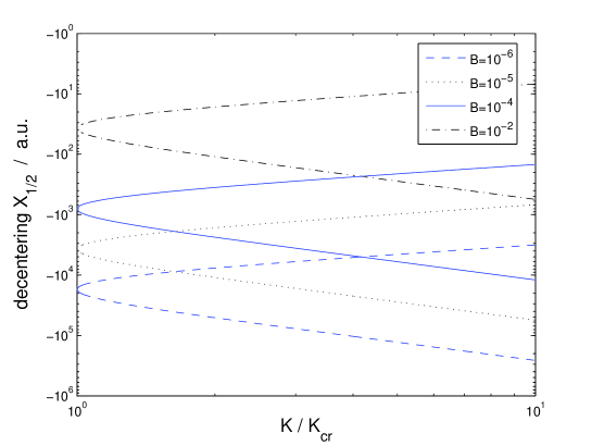
Figure 1: The extremal component $X_{1/2}$ as a function of $K/K_{cr}$ for different field strengths $B/\mathrm{a.u.}$ The critical point $X(K_{cr})$ corresponds to the vertex where $X_{1}$ (lower graph) and $X_{2}$ (upper graph) meet.

For stronger magnetic fields, in turn, the ‘decentering region’ around $X_{c}$ shrinks. We remark that the decentering is virtually insensitive to the number of electrons, $N$.

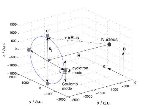
Figure 2: A giant-dipole configuration for $N=4$ electrons ($B=10^{-4},\,K=2K_{cr}$). The ECM $\mathbf{R}=(X,0,0)$ is decentered, with the relative vectors $\mathbf{s}_{i}$ confined to a circle as indicated. Also shown is the electronic vector relative to the nucleus $\mathbf{r}_{i}=\mathbf{R}+\mathbf{s}_{i}$. A typical example of the cyclotron and the motion due to a Coulomb mode is indicated (see Subsec. IV.2.1).

Let us now wrap up our results. Every stationary electronic vector possesses the orthogonal decomposition

$$\mathbf{r}_{i}=X\boldsymbol{\xi}+s(0,\cos\phi_{i},\sin\phi_{i})^{T}.$$

This means that all electrons have a common position along $\boldsymbol{\xi}$—which we refer to as the decentering—while they are confined to a highly symmetric circular configuration perpendicular to $\boldsymbol{\xi}$. This circular configuration in turn is determined only up to an overall rotation $\Delta$. A generic setup is shown in Figure 2.

The extremal solution exists only if the effective pseudomomentum $K^{\prime}$ (controlled via the electric field) exceeds some critical value. The more it does so, the more distinct the decentering of the ECM will be.

IV Normal-mode analysis of $N$-electron giant dipole states

As argued in the previous section, we expect the stationary configurations to be candidates for giant dipole resonances with certain lifetimes. Preceding a numerical study, we first seek to obtain some insight into the local stability of the system, i.e., their behavior in the vicinity of the extrema. To that end, we will carry out a normal-mode analysis about these points. More specifically, we shall consider the harmonic system

$$V(Q) := \mathcal{V}(Q_{0})+\frac{1}{2}(Q-Q_{0})^{T}w(Q-Q_{0}),$$

with the Hessian matrix $w\equiv\partial^{2}\mathcal{V}(Q_{0})\in\mathbb{R}^{3N\times 3N}$. According to Ehrenfest’s theorem, in this case the expectation values $\langle Q\rangle(t)$ obey the corresponding classical equations of motion. Their solution leads us to a quadratic eigenvalue problem, which will be solved by linearization so as to obtain the eigenmodes and -vectors, giving an insight into both the dynamics and the spectrum of the problem.

IV.1 Equations of motion

Before stating the equations of motion, we are to deduce the form of the Hessian matrix of the generalized potential $\mathcal{V}.$ Using the obvious notation

$$(\partial^{2}\mathcal{V})(Q_{0}) = \left(\begin{array}[]{cc}\frac{\partial^{2}\mathcal{V}}{\partial\mathbf{R}\partial\mathbf{R}}&\frac{\partial^{2}\mathcal{V}}{\partial\mathbf{R}\partial\mathbf{s}_{j}}\\ \frac{\partial^{2}\mathcal{V}}{\partial\mathbf{s}_{i}\partial\mathbf{R}}&\frac{\partial^{2}\mathcal{V}}{\partial\mathbf{s}_{i}\partial\mathbf{s}_{j}}\end{array}\right)_{Q_{0}}=\left(\begin{array}[]{cc}w_{RR}&w_{Rj}\\ w_{iR}&w_{ij}\end{array}\right)_{i,j=1}^{N-1},$$

a lengthy calculation reveals that the symmetric matrix $w$ has the the $3\times 3$ block structure

$$w_{RR} = \frac{(NeB)^{2}}{M}I^{\perp}+(Ne)^{2}\left(\frac{I}{r^{3}}-\frac{3}{r^{5}}\left\{\mathbf{R}\otimes\mathbf{R}+\frac{1}{N}\sum_{a=1}^{N}\mathbf{s}_{a}\otimes\mathbf{s}_{a}\right\}\right)$$ (17)

$$w_{Ri} = -Ne^{2}\frac{3}{r^{5}}\left(2\mathrm{S}\left\{(\mathbf{s}_{i}-\mathbf{s}_{N})\otimes\mathbf{R}\right\}+\mathbf{s}_{i}\otimes\mathbf{s}_{i}-\mathbf{s}_{N}\otimes\mathbf{s}_{N}\right)$$

$$w_{ij} = -Ne^{2}\frac{3}{r^{5}}\left(\mathbf{R\otimes R}(1+\delta_{ij})+2\mathrm{S}\left\{(\mathbf{s}_{i}\delta_{ij}+\mathbf{s}_{N})\otimes\mathbf{R}\right\}+\mathbf{s}_{i}\otimes\mathbf{s}_{i}\delta_{ij}+\mathbf{s}_{N}\otimes\mathbf{s}_{N}\right)+$$

$$Ie^{2}\left(N\frac{1+\delta_{ij}}{r^{3}}-\left\{\delta_{ij}\sum_{{{a=1\atop(a\neq j)}}}^{N}s_{aj}^{-3}-(1-\delta_{ij})s_{ij}^{-3}+s_{iN}^{-3}+s_{jN}^{-3}++\sum_{k<N}s_{kN}^{-3}\right\}\right)+$$

$$3e^{2}\Big{(}\delta_{ij}\sum_{{{a=1\atop(a\neq j)}}}^{N}\frac{(\mathbf{s}_{j}-\mathbf{s}_{a})\otimes(\mathbf{s}_{j}-\mathbf{s}_{a})}{s_{ja}^{5}}+\sum_{k<N}\frac{(\mathbf{s}_{N}-\mathbf{s}_{k})\otimes(\mathbf{s}_{N}-\mathbf{s}_{k})}{s_{Nk}^{5}}+$$

$$\left[\frac{(\mathbf{s}_{i}-\mathbf{s}_{N})\otimes(\mathbf{s}_{i}-\mathbf{s}_{N})}{s_{iN}^{5}}+(i\rightarrow j)\right]-(1-\delta_{ij})\frac{(\mathbf{s}_{i}-\mathbf{s}_{j})\otimes(\mathbf{s}_{i}-\mathbf{s}_{j})}{s_{ij}^{5}}\Big{)},$$

where $I^{\perp}\equiv\mathrm{diag}(1,1,0)$, $\mathrm{S}$ denotes the symmetrizer: $\mathrm{S}\{A\}=\frac{1}{2}(A+A^{T})$, and [$\otimes$] represents the tensor product. (All coordinates here of course refer to the extremal positions.)

Despite this rather involved form, the equations of motion themselves look fairly simple:

$$\mu_{N}\ddot{\mathbf{R}} = q\dot{\mathbf{R}}\times\mathbf{B}-w_{R}\cdot(Q-Q_{0})$$

$$m\ddot{\mathbf{s}}_{i} = e\dot{\mathbf{s}}_{i}\times\mathbf{B}-\left(w_{i}-\frac{1}{N}\sum_{k}w_{k}\right)\cdot(Q-Q_{0}).$$ (18)

Here a mixed notation was employed for clarity: $w_{a}\equiv(w_{aR},\,w_{a1},\dots,w_{a,N-1})\in\mathbb{R}^{3\times 3N}$ is the $a$-th block row of $w$. It is inviting to interpret these equations as the motion of effective particles with masses $\mu_{N},\,m$ and charges $q,\,e$, respectively, in a magnetic field, coupled via linear forces.

To solve the equations of motion, let us first write the above system in a more compact way in terms of the displacements $v(t):=Q(t)-Q_{0}$,

$$\ddot{v}=\omega\cdot\dot{v}+A\cdot v.$$ (19)

Here the antisymmetric cyclotron matrix $\omega$ and the harmonic matrix $A$, respectively, have been introduced:

$$\omega = \frac{qB}{\mu}\varepsilon\oplus\frac{eB}{m}\varepsilon\oplus\dots\oplus\frac{eB}{m}\varepsilon\in\mathbb{R}^{3N\times 3N}$$

$$A = -\left(\begin{array}[]{c}w_{R}/\mu\\ \left(w_{i}-\frac{1}{N}\sum_{k}w_{k}\right)/m\end{array}\right)_{i=1,\dots,N-1}\negthickspace\in\mathbb{R}^{3N\times 3N},$$

where $(\varepsilon)_{ij}:=\varepsilon_{ij3}$ is connected with the Levi-Civita tensor and [$\oplus$] stands for the direct sum. The solution of this $3N$-dimensional second-order system of differential equations (ODE) is given by the span

$$v(t)=\sum_{\rho=1}^{6N}(v_{\rho}e^{\gamma_{\rho}t})c_{\rho}\qquad(v_{\rho}\in\mathbb{C}^{3N};\,\gamma_{\rho},c_{\rho}\in\mathbb{C}),$$ (21)

fulfilling the quadratic eigenvalue equation

$$(\gamma_{\rho}^{2}I-\gamma_{\rho}\omega-A)v_{\rho}=0.$$ (22)

In this respect, our stability analysis amounts to finding the complex eigenvalues $\gamma_{\rho}=:\Gamma_{\rho}+i\Omega_{\rho}$ (whose imaginary parts are frequencies of a vibration about a stable point, and whose real part corresponds to an instability), and the eigenvectors $v_{\rho}$.

The above quadratic eigenvalue problem is solved via linearization, which is entirely equivalent to reducing a second-order ODE to a first-order system. In this fashion one obtains a standard linear eigenvalue problem

$$\mathcal{A}u=\gamma u,$$ (23)

with the linearization matrix

$$\mathcal{A}=\left(\begin{array}[]{cc}0&I\\ A&\omega\end{array}\right)\in\mathbb{R}^{6N\times 6N}.$$

Before we present the results, let us state two general properties of the solutions that can be obtained ahead of a computation:

1. For any eigenpair $(\gamma,v)$ of (22) such that Im$\gamma\neq 0$ , there is another pair $(\gamma^{*},v^{*})$.

2. Let $\langle\omega\rangle_{v}:=v^{\dagger}\omega v$ denote the Rayleigh quotient for an arbitrary matrix $\omega$. Assuming $v$ to be a normalized eigenvector, then for any mode the eigenvalue is given by

   $$\gamma^{\pm}=\frac{1}{2}\left(\langle\omega\rangle_{v}\pm\sqrt{\langle\omega\rangle_{v}^{2}+4\langle A\rangle_{v}}\right),$$

   where in general only one of the roots is in the spectrum.

Firstly, (1.) implies that only one out of two modes is relevant; hence it is widely legitimate to treat the $6N$ modes as effectively $3N$. (2.) tells us where in the complex plane we can expect the eigenmodes to lie. If the problem is elliptic, that is

$$\langle A\rangle_{v}<-\left(\frac{\langle\omega\rangle_{v}}{2}\right)^{2}\;\forall v,$$ (24)

then the solution is imaginary $\gamma=i\Omega$ (since $\omega$ is antisymmetric).

IV.2 Results and discussion

IV.2.1 General Classification

Figure 3: Eigenmodes $\{\gamma_{\rho}\}_{\rho}$ for $N=2$ electrons as a function of the electric field $E\equiv BK/M$ over the range $K/K_{cr}\in[1,10]$ (all modes are imaginary). The three plots refer to the magnetic fields $B=10^{-5},10^{-4},10^{-3}$ (from left to right). Each top horizontal line represents two almost degenerate cyclotron modes. Below, the two Coulomb modes fall off quickly and intersect the CM mode (the nearly horizontal line about four orders below the cyclotron modes).

(a) Case of three electrons

(b) Case of four electrons

(c) Case of five electrons

(d) Case of ten electrons

Figure 4: Eigenmodes $\gamma$ for the cases $N=3$ (a), $N=4$ (b), $N=5$ (c) and $N=10$ (d), as a function of the electric field $E\equiv BK/M$, plotted over the range $K/K_{cr}\in[1,10]$. The magnetic field is $B=10^{-4}$. Imaginary parts appear as solid lines, while points (+) are used for the real parts. The individual modes are assigned just as for Fig. 3, with an extra class of very small decay modes, which fall off twice as fast as the Coulomb lines.

Let us first have a look at the behavior of the modes $\{\gamma_{\rho}(K)\}_{\rho}$ for different $N$ at fixed $B$ (Figures 3, 4). Even though the patterns become increasingly rich and involved with higher $N$, one can see a distinction between the modes regarding their behavior as a function of $K$ (and $B$), their order of magnitude and, more generally, their location in the complex plane.

An analysis of the associated eigenvectors and the criterion for ellipticity, (24), will also allow us to illuminate the modes’ origins. This suggests the following classification of the $3N$ eigenmodes:

• $N$ so-called cyclotron modes corresponding to the cyclotron motion of the effective particles. Their values are exclusively on the scale of the cyclotron frequencies, $\gamma=i\Omega\sim i\frac{|e|B}{m}$

• $N$ Coulomb modes corresponding to the inter-Coulombic motion, with a main contribution from the harmonic matrix $A$. They fall off quickly with $K$, since the decentering $X_{0}$ increases, and so the Coulomb interaction becomes less effective.

• 1 CM mode, roughly reflecting the cyclotron motion of the center of mass , $\Omega\sim\frac{NeB}{M}$ (stemming mostly from the CM-kinetic energy)

• 1 zero mode $(\gamma_{\rho}=0)$ that stems from the rotational invariance of the saddle point with respect to the circular configuration (see Eq. 11)

• $N-2$ modes that will be referred to as decay modes in recognition of the fact that they are predominantly real. They are neither directly related to the cyclotron motion nor to the spectrum of $A$, and their slope is twice as steep as that of the Coulomb modes.

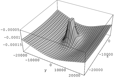
Figure 5: Visualization of the zero mode: plot of the generalized potential $\mathcal{V}$ for $N=2$ close to the extremum, cut along the $yz$ coordinates of $\mathbf{s}$ ($K/K_{cr}=2;B=10^{-4}$). There is a circle that continuously connects all minima, referred to as ‘stationary circle’.

The cyclotron modes roughly pertain to gyrations perpendicular to $\mathbf{B}$, while the Coulomb motion is predominantly parallel to $\mathbf{B}$. The CM mode is primarily a gyrational mode—reflecting the nucleus motion—, but it also exhibits Coulomb-type contributions. The zero mode—to be analyzed in more detail below—corresponds to the rotation along the stationary circle identifiable in Fig. 5. Lastly, the ‘decay modes’ reveal no striking underlying structure.

There are a few subtleties that go beyond the categorization suggested above. A closer look at, for instance, the case of $N=10$ electrons reveals certain interactions among the different modes. Their principal causes are crossings between the center-of-mass mode and the decay modes (resulting in some striking deformations of the usual line pattern), and equally avoided crossings of the CM mode with at least some of the Coulomb modes. This may be taken as a hint at the different symmetry relations among the Coulombic and the decay modes.

IV.2.2 Influence of the rotational invariance $\Delta$

By construction, the stationary character was not affected by a common rotation of the relative coordinates $\mathbf{s}_{a}$ by an angle $\Delta$ on the circle:

$$\mathbf{s}_{a} \mapsto D_{\Delta}\mathbf{s}_{a}\quad\forall a,$$ (25)

$$\phi_{a} \mapsto \phi_{a}+\Delta$$

where $D_{\Delta}\in 1\oplus\mathrm{SO}(2)$ denotes that rotation about the $\boldsymbol{\xi}$ axis. Nonetheless, the Hessian matrix $\partial^{2}\mathcal{V}\big{|}_{Q_{0}}\equiv w$ is affected—and thus the dynamics differs. To see this, note that the block matrices transform like

$$w_{RR} \stackrel{{\scriptstyle D_{\Delta}}}{{\longmapsto}} w_{RR}\;(N>2)$$

$$w_{aj} \stackrel{{\scriptstyle D_{\Delta}}}{{\longmapsto}} D_{\Delta}w_{aj}D_{\Delta}^{-1}.$$

The spectra of both the Coulombic Hessian $(\partial^{2}V)_{0}$ and the magnetic contributions (including $\omega$) are separately invariant under these rotations. Still, their conflicting symmetries guarantee that the dynamics will vary with $\Delta$.

(a) Case of two electrons

(b) Case of three electrons

Figure 6: Upon rotating the circular configuration by an angle $\Delta$, the spectrum is changed in part ($B=10^{-4},\,K=2K_{cr}$). The cyclotronic modes $(658\,\mathrm{GHz})$ and CM mode $(0.17\,\mathrm{GHz})$ remain constant. The Coulomb modes and, for $N=3$, the decay mode ($\sim 10^{-2}\mathrm{GHz}$) show some periodic modulation. (for symbol coding, see Fig. 4)

In order to see this dependency, a semi-log plot of the modes $\{\gamma_{\rho}(\Delta)\}$ on the maximal interval $[0,2\pi)$ is recorded for different $N$ (Fig. 6). As before, $B=10^{-4}$ and $K=2K_{cr}$ are fixed. The plots display an obvious symmetry, as rotating by $\Phi_{N}=2\pi/N$ gives an indistinguishable setup. The cyclotronic modes as well as the affiliated CM mode are essentially $\Delta$-independent. By contrast, the Coulomb modes and the decay modes show a pronounced periodic change. In addition, one can see avoided crossings in some cases between the CM mode and the lowest Coulomb mode.

Figure 7: Spectrum for $N=4$ depending on the rotation angle $\Delta$ ($B=10^{-4},\,K=2K_{cr}$); see text.

For the case $N=2$ (Figure 6a), which was found to be locally stable in the vertical configuration (Schm01, see also IV.2), there is some exceptional behavior whenever $\Delta$ is close to $k\cdot\pi$. The lower Coulomb mode has an avoided crossing with the almost constant CM mode before it experiences a singularity on the logarithmic scale, along the way turning real. In this respect, the local stability we found for $N=2$ is applicable only outside the singular horizontal configuration $\Delta=0$.

While the case of three electrons ($N=3$: Fig. 6b) reveals no striking effects, the spectrum becomes much richer when we add another electron ($N=4$: Fig. 7). The four Coulomb modes as well as two more decay modes reveal an intriguing behavior. There is an avoided crossing between the CM mode and the lowest Coulomb mode, which turns into an unstable real mode in an intermediary region. Also, one can get a sense of the interplay between the two decay modes.

V Wave-packet dynamical study of the two-electron case

The extensive analysis of the normal modes of $N$-electron giant dipole states in the preceding section provided evidence that the two-electron case is locally stable, apart from the singular horizontal configuration. We now turn to a numerical study of that system.

It cannot be over-emphasized that a six-dimensional resonance study is at the frontier of what is currently possible and requires a careful choice of the computational approach. This applies especially in view of the fact that the system is governed by dramatically different time scales. Therefore we adopted the Multi-Configuration Time-Dependent Hartree (mctdh) method mey90:73; bec00:1; mey03:251; mctdh:package, which is known for its outstanding efficiency in high-dimensional applications. To be self-contained, a concise introduction to this tool is presented in Subsection V.1. Its basic idea is to solve the time-dependent Schrödinger equation in a small but time-dependent basis related to Hartree products. It has to be stressed that this method is designed for distinguishable particles. Applying it to a fermionic system like ours finds its sole justification in the fact that the spatial separation between the electrons is so large that they are virtually distinguishable.

After some remarks on the scales of the system in Subsec. V.2, the method will be applied in Subsec. V.3. The focus is on stability aspects, i.e., the propagation of wave packets, but we also investigate the spectra as well as the influence of the rotational invariance discussed in the previous section.

V.1 Computational method: mctdh

The principal goal of mctdh is to solve the time-dependent Schrödinger equation as an initial-value problem:

$$\left\{\begin{array}[]{c}i\dot{\Psi}=H\Psi\\ \Psi(Q,0)=\Psi_{0}(Q)\end{array}\right..$$ (26)

The standard method (see mey03:251 and references therein) now approaches the problem by expanding the solution in terms of time-independent primitive basis functions. Unfortunately, it exhibits a drastic exponential scaling with respect to the number of degrees of freedom $f$. Rather than using a large time-independent basis, the Multi-Configuration Time-Dependent Hartree method (mctdh) employs a time-dependent set, which is more flexible and thus smaller. The ansatz for the wave function now reads

$$\Psi(Q,t)=\sum_{j_{1}=1}^{n_{1}}\ldots\sum_{j_{f}=1}^{n_{f}}A_{j_{1}\ldots j_{f}}(t)\prod_{\kappa=1}^{f}\varphi_{j_{\kappa}}^{(\kappa)}(Q_{\kappa},t)\equiv\sum_{|J|\leq|n|}A_{J}(t)\Phi_{J}(Q,t),$$

using a convenient multi-index notation for the configurations, $J=(j_{1}\dots j_{f})$, where $f$ denotes the number of degrees of freedom. The (unknown) single-particle functions $\varphi_{j_{\kappa}}^{(\kappa)}$ are in turn represented in a primitive basis. Note that both the coefficients $A_{J}$ and the Hartree products $\Phi_{J}$ carry a time-dependence; hence the uniqueness of solutions can only be ensured by adding certain constraints on the single-particle functions bec97:113; bec00:1. Using the Dirac-Frenkel variational principle dir30:376, one can derive equations of motion for both $A_{J,}\,\Phi_{J}$ bec97:113; bec00:1. Integrating these ODE systems allows us to obtain the time evolution of the system, $\Psi(\cdot,t)=\sum_{J}A_{J}(t)\Phi_{J}(\cdot,t)$, which lies at the heart of wave-packet propagation.

The Heidelberg mctdh package mctdh:package, which we used, incorporates a few extensions to this basic concept:

• Product representation of the potential: in order to circumvent multi-dimensional integration in computing the matrix elements, mctdh makes the requirement

  $$H=\sum_{r=1}^{s}c_{r}\prod_{\kappa=1}^{f}h_{r}^{(\kappa)}\,,$$ (27)

  enforcing that the numerical Hamiltonian be written as a sum of products of one-particle operators (separable form). The non-separable part of the Hamiltonian thus has to be fitted to product form ahead of a computation.

• Mode combination: in practice, one combines several (say $d=2,3$) degrees of freedom to a $d$-particle rather than a one-particle function. This approach alleviates the bad numerical scaling for high-dimensional systems.

• Relaxation kos86:223: mctdh provides a way to not only propagate a wave packet, but also to obtain the lowest eigenstates of the (discretized) system. The underlying idea is to propagate some wave function by the non-unitary time-evolution operator $e^{-H\tau}$ (propagation in imaginary time.) In practice, one relies on a more sophisticated scheme termed improved relaxation. Here $\langle\Psi|H-E|\Psi\rangle$ is minimized with respect to both the coefficients $A_{J}$ and the configurations $\Phi_{J}$. The equations of motion thus obtained are then solved iteratively by first solving for $A_{J}(t)$ (by diagonalization of $(\langle\Phi_{J}|H\Phi_{K}\rangle)$ with fixed $\Phi_{J}$) and then propagating $\Phi_{J}$ in imaginary time over a short period. The cycle will then be repeated.

• Spectrum: one can also extract information on the spectrum by computing the auto-correlation function $c(t):=\langle\Psi_{0}\mid e^{-iHt}\Psi_{0}\rangle.$ In the case of a purely discrete spectrum, its Fourier transform reads

  $$\tilde{c}(E)=2\pi\langle\Psi_{0}\mid\delta(H-E)\Psi_{0}\rangle=2\pi\sum_{J}\delta(E_{J}-E)|c_{J}|^{2},$$ (28)

  that is, all eigen-energies give a peak-type contribution, weighted according to the overlap $c_{J}$ of $\Psi_{0}$ with the $J$-th eigenstate.

V.2 Application of mctdh

Let us point out how the computational method can be applied to our problem. There are essentially two highly conflicting types of motion and corresponding scales: perpendicular to the magnetic field, we have the magnetic length

$$R_{B} = \frac{1}{\sqrt{\mu\omega_{B}}}\simeq\frac{1}{\sqrt{2B}},$$

employing atomic units. To be specific, for a laboratory field strength $B=10^{-4}$, the length scale will be on the order of $10^{2}$ a.u. As for the parallel (Coulomb) motion—expected to take place roughly in a harmonic potential—we can use the usual harmonic-oscillator lengths $Z_{0}=1/\sqrt{\mu\omega_{Z}}$, for some ‘typical’ frequency $\omega_{Z}$. These are roughly on the order of $10^{3}$ a.u. (Note that the higher $K$—or $E$— becomes, the smaller will be the Coulomb frequencies, hence the wave packet will be spread far more over the grid.)

Analogously, the anticipated time scales are

$$T_{B}=\frac{2\pi}{\omega_{B}}\stackrel{{\scriptstyle B=10^{-4}}}{{\simeq}}1.5\,\mathrm{ps}$$

for the cyclotronic motion. By contrast, the characteristic times parallel to B are strongly $K$-dependent, and they vary between about $1,500\mathrm{ps}-15,000\mathrm{ps}$. For comparison, we mention that the associate time scale for the CM mode is asymptotically $T_{CM}\simeq 5,000\,\mathrm{ps}$.

For strong fields, the relevant motion will thus certainly be determined by the magnetic field—at least near the stationary points we are interested in. This would suggest to introduce cylindrical coordinates about the extremum, carrying out our study in the basis set for the Landau orbitals landau $R_{nm}(\rho)e^{im\varphi}$ perpendicular to $\mathbf{B}$, and harmonic-oscillator functions $\phi_{n_{z}}(z)$ parallel to the field. Since the former set was not available in the mctdh package, we resorted to Cartesian coordinates for the displacements from the extremum $Q_{0}$ as a pragmatic solution:

$$\mathbf{s}\mapsto\mathbf{s}-\mathbf{s}_{0}\equiv(x,y,z),\quad\mathbf{R}\mapsto\mathbf{R}-\mathbf{R}_{0}\equiv(X,Y,Z).$$

The Hamiltonian (6-7) for our case, centered about the extremum $Q_{0}$ by the generalized translation operators $\exp i(\mathbf{k}_{R}\cdot\mathbf{R}_{0}+\mathbf{k}_{s}\cdot\mathbf{s}_{0})$, reads:

$$\mathcal{T} = -\frac{1}{2\mu}\nabla_{R}^{2}+\frac{1}{8}\mu\omega_{R}^{2}(X^{2}+Y^{2})+\frac{\omega_{R}}{2}L_{Z}+$$

$$-\frac{1}{4m}\nabla_{s}^{2}+\frac{1}{4}m\omega_{s}^{2}(x^{2}+y^{2})+\frac{\omega_{s}}{2}\ell_{z}$$

$$\mathcal{V} = \frac{1}{2M}\left((2eB)^{2}\left[X^{2}+Y^{2}\right]+2X\cdot(X_{0}(2eB)^{2}-2eBK^{\prime})\right)+V_{0}+V_{1}+V_{2}+\mathcal{C}$$

where $\omega_{R}=|q|B/\mu,\,\omega_{s}=|e|B/m$. $\mathcal{C}=\frac{1}{2M}(\mathbf{K^{\prime}}-2e\mathbf{B}\times\mathbf{R}_{0})^{2}$ only shifts the energy by a constant and will be ignored hereafter, and $r_{0}=\tilde{\alpha}|X_{0}|,\,s_{0}=r_{0}/\alpha,\,\phi_{0}=\pi+\Delta$ denote the extremal configuration. Moreover, $V_{0}$ stands for the electron-electron repulsion, whereas $V_{1/2}$ denotes the attractive potentials between the nucleus and electron #1 and #2, respectively. Both $\mathcal{T}$ and the ‘CM-kinetic energy’ are already in product form (27), whereas the Coulomb terms have to be fitted.

V.3 Results and discussion

In our calculations, we were chiefly interested in two questions: the stability of the giant dipole states, and their spectral properties. The first aspect was studied using propagation of wave packets initially localized at the extremum. Emphasis was placed on initial states close to the assumed ‘ground states’. Moreover, following the evolution of wave packets with an initial displacement from the extremum, we tested the robustness of the resonances. For comparison, the eigenvectors of the Hamiltonian will be considered using the relaxation method.

The parameter set was restricted to the following values. $B=10^{-4}$ was fixed, because changing the magnetic field strength essentially only affects the overall scales via the critical pseudomomentum and is not expected to make for completely new behavior. The pseudomomenta are $K/K_{cr}\in\{1.1,\,2.0,\,10.0\}$ (we will drop the prime from now on), which account for the cases of a very shallow outer well, the medium range and the very deep outer well (the high-$K$ regime).

For simplicity, the influence of the rotational invariance will be scrutinized a posteriori, using the characteristic values $\phi_{0}=\frac{\pi}{2},\,\frac{3\pi}{4},\,\pi$. These refer to the vertical configuration ($\Delta=-\frac{\pi}{2}$) first studied in Schm01, a ‘diagonal’ one $\Delta=-\frac{\pi}{4}$, and the horizontal configuration $\Delta=0$, which we expect to have an instability according to the analysis in IV.2.2.

The propagation times were chosen in the regime of $5-10\times 10^{4}\,\mathrm{ps}$. This includes many periods of the Coulomb modes and several $10,000$ periods of the rapid cyclotron motion.

V.3.1 Stability analysis

The approach used in this subsection is to study the propagation of a 6D harmonic-oscillator wave packet centered within the well. The oscillator parameters are adapted so as to match the borderline ground states, i.e., the cyclotron frequencies $\omega_{R},\,\omega_{s}$ for $XY(xy)$, and a typical Coulomb frequency $\omega_{Z},\,\omega_{z}$ parallel to the magnetic field. To test the robustness of the potential resonance, in some cases displacements of $\langle Z\rangle_{0}=\langle z\rangle_{0}=2000$ a.u. are also applied to the initial wave function. (This value is arbitrary but moderate compared to the total decentering.) Also, relaxations (starting from the original, undisplaced wave packets above) are carried out to see how the lowest-energy configuration found with this algorithm differs from our initial guess. The analysis mostly focuses on the reduced densities $\rho_{\kappa}$ (1D or 2D) obtained by integrating out all but the $\kappa$-th degree(s) of freedom. Where appropriate, the wave packets’ centers and widths $\langle q_{\kappa}\rangle(t),\,\Delta q_{\kappa}(t)$ are shown.

The case $K=1.1K_{cr}$:

Very close to the critical point, $K_{cr}$, the observed motion displays an instability in some degrees of freedom.

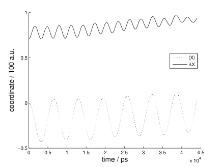
Figure 8: The motion in $X$ in the case $K/K_{cr}=1.1$
(a) Snapshots of the motion $\rho_{X}$, reflecting oscillations of both center and shape of the wave packet
(b) The two oscillations as documented in $\langle X\rangle(t),\,\Delta X(t)$

Both $X$ and $Y$ revealed weak oscillations of two types. As these are generic, they shall be inspected in more detail on the example of the $X$ degree of freedom. Three representative snapshots (Figure 8a) were taken to illustrate this effect. The nature of the oscillations can be explored more easily in Figure 8(b). To begin with, the center carries out a tiny oscillation about $X\simeq-20$ a.u. with a period of about $6,400\,\mathrm{ps}$ (a snapshot was taken at its first turning point at $3,200\,\mathrm{ps}$). This very slow oscillation superimposes what we will call the shape oscillations, materializing in the fluctuation of the width $\Delta X(t)$. That oscillation is about twice as fast, and it reaches its maximum width for the first time at $1,600\,\mathrm{ps}$ (Fig. 8a). The relative stability in these two directions is readily explained in terms of the generalized potential. Apart from a stabilization by the $\mathbf{B}$ field, they experience an additional confinement via the ‘CM-kinetic energy’ (5). However, it is evident that the packet broadens over time, thus slowly delocalizing (Fig. 8b).

Figure 9: Cuts through the generalized potential near the extremum,$\mathcal{V}(X,Y,0;\mathbf{0})$ (a) and $\mathcal{V}(\mathbf{0};x,y,0)$ (b), exemplified for $K=1.1K_{cr}$. The $(XY)$ potential is almost harmonic. The $y$ direction virtually coincides with the zero mode, whereas the potential exhibits an instability with respect to $x$.

(a) Cut through the Z direction

(b) Cut through the z direction

Figure 10: Cuts through the generalized potential parallel to the magnetic field: (a) $\mathcal{V}(0,0,Z;\mathbf{0})$ is roughly harmonic, (b) $\mathcal{V}(\mathbf{0};0,0,z)$ is strongly flattened on the right-hand region of the minimum. (Note that the extremum is shifted to the origin.)

Even though the relative motion perpendicular to B, $\mathbf{s}_{\perp}\equiv(x,y)$, is also gyrationally stabilized, there is no confining term for it in the generalized potential as for the ECM. In fact, a look at the generalized potential (Figure 9b) reveals that $Q_{0}$ is a saddle point. The $y$ direction is the zero mode, while the cut through the $x$ direction refers to a maximum. In this light, we cannot expect the system to be arbitrarily stable in these two degrees of freedom. This is a general fact, but for $K=1.1K_{cr}$ it is very pronounced. The reason being, near the extremum, the Coulomb interaction (the source of these instabilities) becomes negligible for higher $K$. A line of reasoning closely connected uses the time scale at which the instability will have an impact. As the Coulomb modes $\Omega(K)$ increase dramatically as $K\rightarrow K_{cr}^{+}$, their characteristic time $T(K)=2\pi/\Omega(K)$ becomes much shorter (cf. Table 1).

$K/K_{cr}$	$T_{\mathrm{C}}(K)$	$|X_{0}(K)|$
1.1	$.1-.4\,\mathrm{ns}$	$1.4\cdot 10^{4}\,\mathrm{a.u.}$
2	$.4-1\,\mathrm{ns}$	$2.9\cdot 10^{4}\,\mathrm{a.u.}$
10	$5-15\,\mathrm{ns}$	$1.5\cdot 10^{5}\,\mathrm{a.u.}$

Table 1: Summary of time scale of the Coulomb motion $(T_{\mathrm{C}})$ and length scale $(|X_{0}|)$ for different values of pseudo-momentum $K$

Figure 11: Snapshots of the wave packet’s motion in the direction of $x$ (a), $y$ (b) and $z$ (c) for $K=1.1K_{\mathrm{cr}}$. The plots display the reduced densities $\rho_{x}$, $\rho_{y}$ and $\rho_{z}$ at different times. While the unstable mode $x$ leaks slowly, the zero mode $y$ spreads much more quickly. The wave packet in $z$ is only marginally shifted over time. In (d), the different oscillations in $z$ are illustrated.

These considerations shed light on Figure 11. For instance, $\rho_{x}$ soon develops two small side maxima. They become more pronounced as time goes on and slowly spread towards the boundary of the grid. The zero mode ($y$) spreads out much faster—that is, to a significant extent after 2,000 ps already.

Figure 12: The motion of the $Z$ mode in the case $K/K_{cr}=1.1$. Three snapshots of the reduced density $\rho_{Z}$ are plotted.

The reduced density for $Z$ (Fig. 12) broadens and continually leaks toward the grid ends. Although in the $Z$ direction, the particle lives in a fairly harmonic well (Fig. 10), it is not only lifted in energy to way above the bottom of the well, but also affected by the instability in $x$ via coupling. Turning to the last degree of freedom, $z$, we find an overall stable behavior. Note that there is an overlay of a fast but tiny oscillation of the packet’s center and a slower and less regular one visible in Figure 11(d) as the envelope of $\langle z\rangle(t)$.

The case $K=2K_{cr}$:

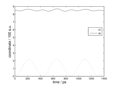
Figure 13: The expectation values and uncertainties over selected time periods for the coordinates (a) $Z$ and (b) $z$ ($K/K_{cr}=2$).

For $K$ being twice its critical value, the vertical configuration is virtually stable on a scale of $T\sim 10^{4}\,\mathrm{ps}$. The degrees of freedom $X$ and $Y$, as well as the parallel motion $Z$ and $z$, turn out to be indeed perfectly stable. Again, there are two different types of tiny oscillations, displayed in Figure 13, which are fingerprints of the coupling with the Coulombic motion (indicated by plotting $\langle q_{\kappa}\rangle(t)$ over some periods $T_{Z}$, for instance).

Figure 14: The relative coordinate $\mathbf{s}_{\perp}$ in the case $K/K_{cr}=2$: Characteristic snapshots of the reduced density $\rho_{y}$.

As opposed to the previous paragraph $K/K_{cr}=1.1$, the relative motion in $x$ conveys a fairly stable if erratic impression. Still, the wave packet in $y$ spreads as it did before (Fig. 14). But keep in mind that it occurs at a much greater time scale than in Fig. 11(b): for example, after 5,000 ps the broadening has only just begun to become significant.

A closer look at the response of the system upon displacing $Z$ and $z$ by $2,000\,\mathrm{a.u.}$ unveils that for the excited degrees themselves, $Z$ and $z$, the wave packet is simply reflected between two positions $\pm\langle z\rangle_{0}$ with minor ($Z$) or more pronounced ($z$) deformations and smearing-out due to competing modes, cf. Figure 15(a-b). The most interesting question may be the effect on the $(xy)$ modes. In fact, $x$ is rendered slightly unstable by the excitation of the parallel motion. The snapshots taken at 20,000 ps and 50,000 ps, respectively, document how the wave packet slowly but inevitably starts leaking, Fig. 15(c-d). The lifetime of the $y$ mode is not drastically changed altogether.

Figure 15: Snapshots of the wave-packet upon an initial displacement by $Z=z=2,000\,\mathrm{a.u.}$ for $K/K_{cr}=2$. Plot (a) illustrates the strong deformations in $Z$ in the course of the oscillation; (b) shows how the the $z$ packet is distorted after several thousand pico-seconds. The non-stable modes $x,y$ are affected via coupling, see (c) and (d).

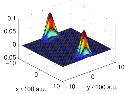
Figure 16: A generic relaxation state ($K=2K_{cr}$, see text) – plotted is the 2D-reduced density for the plane perpendicular to $B$: the wave packet is driven away from the $x$ axis with increasing basis size.

We also investigated the supposed ground state obtained via improved relaxation. It is understood that at best the exact system displays a resonance state, so the quest for eigenstates is meaningful only insomuch as those of the discretized Hamiltonian may be interpreted as localized states which really correspond to resonances. Our results turned out to be very sensitive to both the primitive and the single-particle basis sizes. Nonetheless, for a high if manageable accuracy, the pattern that emerged was the following. Apart from some smaller deviations from the initial state (Landau-orbital / harmonic-oscillator product), a drastic alteration takes place in $\mathbf{s}_{\perp}\equiv(x,y)$ (Fig. 16). The wave packet is split into two humps that seem to be driven outwards until the basis size is exhausted, while smeared out along the zero mode $y$.

This behavior raises the question how that squares with the potential picture, given that the local instability characterized by $\omega_{x}^{2}\equiv w_{xx}/m$ is much weaker in magnitude than $\omega_{B}^{2}$. In order to clarify these issues, we constructed a 2D model Hamiltonian via the natural inclusion $H_{xy}:=H\!\mid_{\mathbf{R}=\mathbf{0};\,z=0}$. The study of this toy model, which is numerically far more amenable, revealed that it is capable of recovering many of the key features of the full system. It therefore provided a valuable tool in detecting the key to this mechanism—the paramagnetic term $\omega_{B}\ell_{z}$. To begin with, the instability of the generalized potential in $x$ tempts the packet to split up and be driven ‘downhill’. However, if there were no paramagnetic term or if the same instability occurred isotropically, this would have no discernible effect. However, owing to the anisotropy of $\mathcal{V}$, $\boldsymbol{\ell}$ is no longer conserved:

$$\dot{\boldsymbol{\ell}}=-\mathbf{s}\times\nabla\mathcal{V}.$$

It is energetically favorable for the particle to go to ever lower $\langle\ell_{z}\rangle<0$ while being expelled from the unstable line $x=0$, thus introducing a high correlation between $x$ and $y$.

Note that this effect essentially amounts to the fact that the giant-dipole resonance state is far from the energetically lowest configuration. That does not pose an immediate constraint on the system’s lifetime under propagation, since our initial Landau/harmonic-oscillator state has a virtually zero overlap with the above ‘relaxation state’. Hence in a propagation, this ‘bimodal’ relaxation state is not accessible, which explains why the system is so much more stable than its relaxation suggests. Physically speaking, the cyclotron gyration field stabilizes the motion near the stationary configuration for fixed energy and thus inhibits a delocalized state at a lower energy. – This is approved by a 2D numerically exact time evolution (Fig. 17), which reveals no breakup for many nanoseconds, until the wave packet is slightly rotated in the $xy$ plane and split up roughly in the $y$ direction—and not in $x$ as in the relaxation case! Note that it acquires a small but non-zero value of $\langle\ell_{z}\rangle\sim-1$, in contrast to $\langle\ell_{z}\rangle\sim-60$ in Fig. 16; this also reflects the higher level of stability. It is only after way more than $100\,\mathrm{ns}$ that the packet hits the grid’s boundary. These outcomes seem to confirm that for moderate values of $K$, our system is quasi-stable on a time scale of up to $T\sim 100\,\mathrm{ns}$.

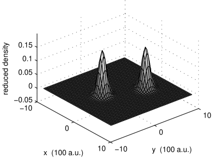
Figure 17: Wave packet of the 2D model ($xy$) after $T=160\,\mathrm{ns}$ ($K=2K_{cr}$, see text)

The case $K=10K_{cr}$:

For this value, which corresponds to $E\equiv BK/M=207\,\mathrm{\frac{kV}{m}}$, we find the system to be practically stable on the time scale we considered, $T=100\,\mathrm{ns}$.

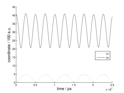
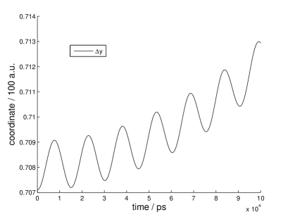
Figure 18: The time evolution of $\langle z\rangle,\Delta z$ (a) and $\Delta y$ (b) for $K/K_{cr}=10$. Both degrees are altogether stable, but oscillate due to coupling. A marginal broadening can be seen in $y$.

The initial wave packet experiences only tiny deformations in most degrees of freedom, which are not discussed here. However, there are oscillations for $z$, which are more pronounced but still marginal compared to the spatial extension of the decentered state; these are sketched in Figure 18(a). While its center shows a shift to positive values of $z$, its elongation is on the order of $250\,\mathrm{a.u.}$, and the width varies by a factor of two, all at a period of about $T_{z}$. In contrast with $x$ and any other degree, the width in the $y$ direction shows a steady if minute broadening (Fig. 18b). This might be taken for a sign that eventually, the system is bound to decay. Then again, this takes $300,000\,\mathrm{ps}$ to move by one atomic unit and is beyond the time scale regarded here.

After having come a long way to find the system practically stable for high enough values of the pseudo-momentum, we now explore the robustness with respect to displacements. Skipping the detailed behavior, we find that the overall stability was not affected. Due to coupling to other modes, the excitation of the parallel motion imprints some oscillations both of the packet’s center and its width on the perpendicular degrees of freedom.

Lastly, applying a relaxation revealed similar phenomena as in the previous paragraph. Regardless of the specific shape of the relaxation state, it can be reasoned that the instabilities of course still underlie the system, but that the lifetimes for sufficiently large $K$ are too large to be observed in our propagation.

V.3.2 Influence of the rotational freedom

To complete the discussion, let us now investigate the giant dipole states for different settings of the extremal angle $\phi_{0}$ of the relative coordinate $\mathbf{s}_{0}$ on the circle. So far, the focus was on $\phi_{0}=\pi/2$ only (or, equivalently, $\Delta=-\frac{\pi}{2}$), which we referred to as the ‘vertical configuration’. In the normal-mode analysis, however, we found an interesting frequency pattern as we varied this extremal angle. It was argued that each $\phi_{0}$ corresponds to a different extremal point, i.e., for each value of $(B,K)$ there is really a one-parameter class of extremal points $Q(\phi_{0})$ with different stability and spectral properties.

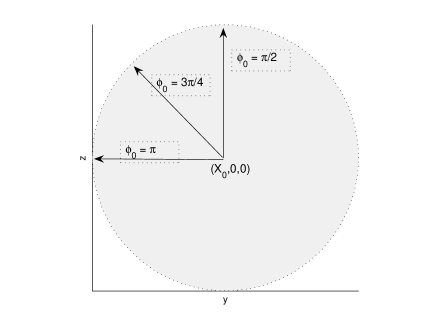
Figure 19: The circular configuration $\mathbf{s}^{(0)}=s_{0}(0,\cos\phi_{0},\sin\phi_{0})^{T}$ for $N=2$, depending on the angle $\phi_{0}$. The arrows refer to $\mathbf{s}^{(0)}$ in the $yz$-plane for different values of $\phi_{0}$. The $X$ axis points into the page.

As examples, we thus investigate both the supposedly unstable ‘horizontal configuration’ $\phi_{0}=\pi$ $(\Delta=0)$ and a ‘diagonal configuration’ $\phi_{0}=\frac{3}{4}\pi$ $(\Delta=-\pi/4)$, as visualized in Figure 19. This was done for the special cases of $K/K_{cr}=2,\,10.$

To sum up our findings, the horizontal configuration indeed adds an instability, which is discernible even for very high $K$, if less distinct. The diagonal configuration was partly unstable on a timescale comparable to that of the vertical case, $T\sim 10^{4}\,\mathrm{ps}$. A rotation of the extremum obviously rotates the zero mode, too, which is why the detailed dynamics is a different one for the relative degrees of freedom. For instance, in case that $\phi_{0}=\pi$, the zero mode points along the $z$ direction, which would otherwise live in a harmonic potential. As a consequence, even for $K/K_{cr}=10$ the $z$-packet (prepared with a non-zero frequency $\omega_{z}=10^{-8}\mathrm{a.u.}$) smoothly oscillates between its initial and a much more smeared-out state according to Fig. 20.

Figure 20: The horizontal configuration $\phi_{0}=\pi\,(K/K_{cr}=10)$. The wave packet switches between two positions (snapshots of reduced density for 11,500 ps and 20,000 ps).

V.3.3 Spectrum

Figure 21: Fourier transform of the auto-correlation function (the ‘spectrum’) for $K/K_{cr}=1.1$.

We finally look into some spectral properties of the GDS for the different values of $K/K_{cr}$. The spectrum calculated from a propagation for $K/K_{cr}=1.1$ (Fig. 21) looks somewhat fuzzy, but the main peak is still distinct enough to vaguely resemble a resonance. The situation is less ambiguous in the case $K/K_{cr}=2$ , as the ‘decay’ occurs on a much greater time scale.

Figure 22: Spectrum for $K/K_{cr}=2$. The dotted peak again belongs to the initial state. For the excited (or displaced) initial state, the spectrum shows a sequence of peaks (here almost equidistant).

The spectrum in Fig. 22 illustrates the resonance character of the system. Our initial wave packet gives a peak at $E\simeq 0.281\textrm{ meV}$, whereas the ‘displaced state’ with $\langle z\rangle_{0}=\langle Z\rangle_{0}=2,000\,\mathrm{a.u.}$ produces a rather interesting excitation spectrum (same figure), revealing overlaps with many eigenstates. The equidistant spacing of the peaks might be interpreted as a signature of harmonicity in both excitations ($Z,\,z$). Finally, in the most stable case $K/K_{cr}=10$, the spectrum consists of a sharp dominant peak at about 2.2422 eV, plus a very tiny one 0.0017 eV above. This somehow quantifies our empirical observation that $K/K_{cr}=10$ is quasi-stable.

VI Conclusion and outlook

We have studied the internal motion of $N$-electron atoms in crossed magnetic and electric fields utilizing the generalized potential. For electric fields above a critical value, a strongly decentered potential well forms. It supports giant dipole states where the electrons’ center of mass is aligned along the electric field, with all electrons in a symmetric circular configuration in the orthogonal plane. These states have been investigated for an arbitrary number of electrons in a normal-mode analysis, and numerically for the case of two-electron giant dipole states employing wave-packet propagation.

The normal-mode analysis of the $N$-electron atoms leads to a quadratic eigenvalue problem. Its eigenmodes (as well as the eigenvectors) have been studied depending on the field strengths $B,\,E$ as well as the electron number $N$. A subsequent classification according to their characteristics indicated that the $3N$ modes were grouped into $N$ cyclotron modes and $N$ Coulomb modes, corresponding mostly to the motion induced by the magnetic field and the Coulomb potential, respectively. Moreover, we found a CM mode reflecting the center-of-mass gyration in the magnetic field, as well as a zero mode referring to a rotational invariance of the extremal configuration, also studied in detail. The residual modes were termed decay modes on account of their peculiar behavior suggesting instability for atoms with three or more electrons. Their absence for the system $N=2$ provided a strong indication of local stability, with the single exception of the so-called horizontal configuration.

In the second part of the present work, an ab-initio simulation of the six-dimensional two-electron system was performed. Since this type of investigation can be viewed as the state of the art of what is numerically feasible, we resorted to the Multi-Configuration Time-Dependent Hartree (mctdh) method, a wave-packet dynamics tool known for its unique efficiency in higher dimensions. Both the stability of the six degrees of freedom and some spectral properties have been examined. To establish the link to the normal-mode analysis, the influence of the rotational freedom of the circular configuration has also been investigated. We find that the stability of the system strongly increases for larger electric fields. For a field strength twice the critical value, some modes experience a decay on the time scale of $10^{4}-10^{5}\,\mathrm{ps}$; for the tenfold critical value, there is no instablity on the scale we considered, i.e., $10^{5}\,\mathrm{ps}$. These states proved rather robust against perturbations, simulated by displacements parallel to the magnetic field, where the motion is not gyrationally stabilized. As anticipated, the stability of the giant dipole states turned out to apply only outside the singular ‘horizontal configuration’ of the extremum.

While the investigation into the local aspects of stability can be regarded as somewhat completed, a rigorous numerical analysis is to date limited with an eye toward time and computational effort. First and foremost, the mctdh calculations set up so far could in principle be modified to the case of $N\geq 3$ electrons. However, this appears to be a massive numerical challenge, since the mctdh method is slowed down significantly the more degrees of freedom are involved. One approach to circumvent this would be an adiabatic separation similar to bezchastnov02, amounting to an average over the rapid cyclotron motion. This would allow for a significantly faster integration. For future investigations, it may also be beneficial for short-time propagations to implement a discrete-variable representation of the Landau orbitals in mctdh.

Apart from these questions, concerned with a wider range of application and efficiency, the task arises to make the analysis more quantitative. A systematic resonance calculation yielding both the energy levels and decay widths of the giant-dipole states is desirable, but has so far proven to be a severe challenge computationally due to the type of instability. It might also yield a deeper understanding of the resonance wave functions. Ultimately, one could even go so far as to simulate the preparation of giant dipole states, migrating from the Coulomb well to the decentered extremum. In analogy to the scheme suggested for single electrons Ave99:3695, this may serve as a bridge to the experimental verification of giant dipole resonances.