On Consistent and Calibrated Inference about
the Parameters of Sampling Distributions

Tomaž Podobnik^1), 2), and Tomi Živko^2),
1)Physics Department, University of Ljubljana, Slovenia

²⁾”Jožef Stefan” Institute, Ljubljana, Slovenia

The theory of probability, based on very general rules referred to as the Cox-Pólya-Jaynes Desiderata, can be used both as a theory of random mass phenomena and as a quantitative theory of plausible inference about the parameters of sampling distributions. The existing applications of the Desiderata must be extended in order to allow for consistent inferences in the limit of complete a priori ignorance about the values of the parameters. Since the limits of consistent quantitative inference from incomplete information can clearly be established, the developed theory is necessarily an effective one. It is interesting to note that when applying the Desiderata strictly, we find no contradictions between the so-called Bayesian and frequentist schools of inductive reasoning.

Ljubljana, August 2005

As for prophecies, they will pass away; as for tongues, they will cease; as for knowledge, it will pass away. For we know in part and we prophesy in part.
1 Corinthians 13, 8-9.

1 Introduction

The term inference ([1], p. 436) stands for two kinds of reasoning ([2], p. xix): deductive or demonstrative reasoning whenever enough information is at hand to permit it, and inductive or plausible reasoning when not all of the necessary information is available. “The difference between the two kinds of reasoning is great and manifold. Demonstrative reasoning is safe, beyond controversy, and final. Plausible reasoning is hazardous, controversial, and provisional. Demonstrative reasoning penetrates the science just as far as mathematics does, but is in itself (as mathematics is in itself) incapable of yielding essentially new knowledge about the world around us. Anything new that we learn about the world involves plausible reasoning, which is the only kind of reasoning for which we care in everyday affairs. Demonstrative reasoning has rigid standards, codified and clarified by logic (formal or demonstrative logic), which is the theory of demonstrative reasoning. The standards of plausible reasoning are fluid, and there is no theory of such reasoning that could be compared to demonstrative logic in clarity or would command comparable consensus.” So George Pólya in the Preface to his Mathematics and Plausible Reasoning ([3], p. v).

In the second volume [4] of the work he collects patterns of plausible reasoning and dissects our intuitive common sense into a set of elementary qualitative desiderata that represent basic rules of inductive reasoning. When formulating his views in mathematical terms ([4], Chapter XV), he recognizes his rules to be in a close agreement with the calculus of probability as developed by Laplace in the late 18th century [5], but Pólya advances a thesis that when applying the calculus of probability to plausible reasoning, it should be applied only qualitatively (see, for example, [4], pp. 136-139), i.e. numerical values should be strictly avoided.

In the present paper we formulate a quantitative theory of inductive reasoning, in particular a consistent theory of quantitative inference about the parameters of sampling distributions. In Section 2 we adopt the basic qualitative rules of plausible reasoning, the so-called Cox-Pólya-Jaynes Desiderata, and review some of the well known results of their direct applications, such as Cox’s and Bayes’ Theorems. In addition, we clearly establish the lack of such applications in the limit of complete prior ignorance about the inferred parameter, with such ignorance representing the natural starting point of an inference. In other words, Bayes’ Theorem that can be used for updating probabilities, cannot directly be used in the step of probability assignment.

We carefully define the state of complete prior ignorance about the inferred parameter in Section 3. In particular, throughout the present paper we never question the specified model, i.e. the form of the sampling probability distribution is always known beyond the required precision. What we are completely ignorant about at the beginning of reasoning is the value of the inferred parameter.

In Section 4 we define location, dispersion and scale parameters and briefly review some of the properties of sampling distributions determined by these parameters. A separate section is devoted to the invariance of such distributions, a property that turns out to be of decisive importance when constructing a consistent theory of inductive reasoning. We also show that invariance of both the form of the sampling distribution and its domain, under a continuous (or Lie) group, is found only in problems of inference about parameters that can be reduced to inference about location parameters.

In Section 6 we extend the applications of the Desiderata in order to allow for a consistent assignment and not just for updating of probability distributions for the inferred parameters. The so-called Consistency Theorem is obtained by making use of Bayes’ Theorem and by requiring that if a conclusion can be reasoned out in more than one way, then every possible way must lead to the same result, in particular by requiring logically independent pieces of information to be commutative. The form of the Consistency Theorem is very similar to that of Bayes’ Theorem, but there is also a fundamental difference between the two since in the former a consistency factor is used instead of the prior probability distribution. Hence, the consistency factor cannot be subject to any of the requirements such as normalization or invariance with respect to a one-to-one parameter transformation, that are perfectly legitimate for well defined probability distributions.

Instead, the form of the consistency factor is determined in a way that preserves the logical consistency of our reasoning. By consistency we mean that, among other things, if in two problems of inference our state of knowledge is the same, then we must assign the same probabilities in both. In Section 7 we find that the basic Desiderata uniquely determine the form of consistency factors for sampling distributions whose form and domain are invariant under a Lie group $\mathcal{G}$ of transformations. It is therefore only for those problems reducible to inference about location parameters that we can give an assurance of consistency to our parameter inference. The form of consistency factors for such distributions is then determined throughout Sections 8-10, while in Section 11 we discuss under what circumstances the present theory is guaranteed to be consistent in the case of pre-constrained parameters.

In Section 12 we make verifiable predictions that are based on the presented theory, thus elevating its status above the level of a mere speculation. The predictions are made in terms of long run relative frequencies. We show that a consistent inference is necessarily also a calibrated one, i.e. that consistently predicted frequencies always coincide with (a one-to-one function of) actual frequencies of occurrence. This important result speaks in favour of a complete reconciliation between the so-called Bayesian and frequentist schools of plausible reasoning.

In counting experiments the invariance of sampling distributions is clearly missing and so the consistency factors cannot be uniquely determined by following the basic Desiderata. The remedy is to collect enough data so that the sampling distribution approaches its dense limit. Until then, our reasoning is necessarily based on some ad hoc prescriptions that can (and very often will) lead to logically unacceptable results, as is demonstrated in Section 14. In such cases it might therefore be the best to refrain from quantitative inferences, i.e. to remain on a qualitative level.

In Section 15 we briefly review conceptual and practical difficulties and paradoxes caused by using Bayes’ Theorem instead of the Consistency Theorem in the limit of complete ignorance about the inferred parameters. The problem is contained in the self-contradicting non-informative prior probability distributions. Long-lasting arguments over this subject led, inter alia, to a split in the theory of inductive reasoning and it is in this way that the Bayesian and the frequentist schools emerged. In our view, the splitting into (at first glance) almost diametrically opposed schools is highly artificial, provided that the two schools strictly obey their basic rules, i.e. that they refrain from using ad hoc shortcuts on the course of inference. For regardless how close to our intuitive reasoning these ad hoc procedures may be, how well they may have performed in some other previous inferences, and how respectable their names may sound (e.g. the principle of insufficient reason or its sophisticated version - the principle of maximum entropy, the principle of group invariance, the principle of maximum likelihood, and the principle of reduction), they will in general inevitably lead not only to contradictions between the two schools of thought, but also to inferences that are neither consistent nor calibrated.

There are also two appendices to the present paper. The first one contains, for the sake of completeness, a proof of Cox’s Theorem, while in the second one, the so-called marginalization paradox, is extensively discussed.

2 Basic rules and their applications

Let n hypothesis or an event be an unambiguous proposition $A$ , i.e. a statement that can be either true or false. As we are in general not certain about either of the two possibilities, the classical logic of deductive reasoning [6] is to be extended in order to allow for plausible or inductive inferences based on incomplete information.

Let (a state of) information $I$ summarize the information that we have about some set $\mathcal{A}$ of propositions $A_{i}$, called the basis of $I$, and their relations to each other. The domain of $I$ is the logical closure of ${\cal A}$, that is, the union of ${\cal A}$. A state of information is not restricted to containing only deductive information; it can also contain imprecise or insufficient information that says nothing with certainty, but still affects one’s opinion about a certain proposition. Such kind of information can also be updated: we write $I^{\prime}=BI$ for a state of information obtained from $I$ by adding additional information ( evidence) that proposition $B$ is true.

Now, let $I$ be a state of information of a given person and $A$ be a proposition in the domain of $I$. Then, we introduce the (degree of) plausibility $(A|I)$ as a degree of belief of the person that $A$ is true given the information in $I$. We say that $I$ is the knowledge base for the assigned plausibility $(A|I)$. In the present paper we assume all considered plausibilities to be subject to very general requirements that can be listed in the following three basic Cox-Pólya-Jaynes Desiderata ([2], § 1.7, pp. 17-19):

I.

Degrees of plausibilities are represented by real numbers.

That is, plausibilities are numerically encoded states of knowledge about propositions. Formally, an assigned plausibility can be regarded as a function:

$$\begin{CD}(\;|\;):{\cal A}\times{\cal I}@>{}>{}>\mathbb{R}\ ,\end{CD}$$

where ${\cal I}$ is the set of possible states of information about some set ${\cal A}$ of propositions.

In addition to the first Desideratum, we adopt two natural but nonessential conventions:

• a greater degree of belief shall correspond to a greater number;

• the plausibility of a hypothesis that we are certain about (e.g. the plausibility of a tautology) equals 1.

By referring to the conventions as being nonessential we mean that we could have equally well adopted a convention that the plausibility of a tautology equals a different positive constant, or that a greater degree of probability should correspond to a smaller number. Nevertheless, according to the above Desideratum and the two conventions, the assigned plausibilities can range within an interval $[{\mathsf{F}},1]$, where ${\mathsf{F}}<1$ is plausibility of the false proposition.

We say that a state of information $I$ is consistent if there is no proposition $A$ for which plausibilities $(A|I)$ for $A$ being true and $(\bar{A}|I)$ for $A$ being false can both equal unity. That is, based on consistent information both a proposition and its denial cannot be true. In order to avoid ambiguities, we restrict ourselves to considering only plausibilities that are assigned upon consistent states of information.

II.

Assignment of plausibilities must be in qualitative correspondence with common sense.

In our case, the concept of common sense stands for the following conditions:

• Since plausible reasoning is a generalization of deductive logic, it must be consistent with the results of Boolean algebra [7] - the algebra of deductive logic.

• Microscopic changes in the knowledge base should not cause macroscopic changes in the plausibilities assigned. In addition, for every considered proposition $A$ there exists some set of possible consistent states of knowledge ${\cal I}$ such that $(A|I)$, with $I\in{\cal I}$, can take any of the values within a continuous interval $(a,b)\subseteq[{\mathsf{F}},1]$ (continuity requirement).

• We assume that the degree of belief $(\bar{A}|I)$ that $A$ is false depends in some way on the plausibility $(A|I)$ that $A$ is true. In addition, when old information $I$ is updated into $I^{\prime}$ in such a way that the plausibility of $A$ is increased, $(A|I^{\prime})>(A|I)$, it must produce a decrease in the plausibility that $A$ is false, $(\bar{A}|I^{\prime})<(\bar{A}|I)$. That is, we assume that there exists a continuous, twice differentiable, strictly decreasing function $S$ of plausibility $(A|I)$, such that

  $$(\bar{A}|I)=S\bigl{[}(A|I)\bigr{]}\ .$$

• Plausibility $(AB|I)$, assigned to a hypothesis $AB$ that two non-contradictory hypotheses, $A$ and $B$ , are simultaneously true, is assumed to be completely determined by the values of $(A|I)$, $(B|AI)$, $(B|I)$ and $(A|BI)$. Then it can be shown (see Lemma 1 in Appendix A) that evident inconsistencies are avoided only if $(AB|I)$ depends solely on $(A|I)$ and $(B|AI)$, i.e. if there exists a function $H$ such that

  $$(AB|I)=H\bigl{[}(A|I),(B|AI)]\ .$$

  We further require for the function $H$ to be strictly increasing and twice differentiable in both of its arguments. By strictly increasing we mean that if the knowledge base $I$ is updated to $I^{\prime}$ in such a way that the plausibility of $A$ is increased, $(A|I^{\prime})>(A|I)$, but the plausibility $(B|AI)$ remains the same, $(B|AI^{\prime})=(B|AI)$, this can only produce an increase in the plausibility that both $A$ and $B$ are true, $(AB|I^{\prime})\geq(AB|I)$, in which the equality can hold only if $B$ is impossible given $A$ and $I$. Likewise, given information $I^{\prime\prime}$ such that $(A|I^{\prime\prime})=(A|I)$ and $(B|AI^{\prime\prime})>(B|AI)$, we require that $(AB|I^{\prime\prime})\geq(AB|I)$.

III.

Assignment of plausibilities must be a consistent procedure:

a)

If a conclusion can be reasoned out in more than one way, then every possible way must lead to the same result.

b)

When assigning plausibilities, we must always take into account all of the evidence we have relevant to a hypothesis. We do not arbitrarily ignore some of the information and base our conclusion only on what remains.

c)

Equivalent states of knowledge must be always represented by equivalent plausibility assignments. For example, if in two problems our state of knowledge is the same (except perhaps for the labelling of the propositions), then we must assign the same plausibilities in both.

The requirement of consistency plays a special rôle among various requirements which a theoretical system, or an axiomatic system, must satisfy. It can be regarded as the first of the requirements to be satisfied by every theoretical system, be it empirical or non-empirical. As for an empirical system, however, besides being consistent, it should satisfy a further criterion: it must be falsifiable ([8], § 24, pp. 91-92). According to this criterion, statements, or systems of statements, convey information about the empirical world only if they are capable of clashing with experience; or more precisely, only if they can be systematically tested, that is to say, if they can be subjected (in accordance with a methodological decision) to tests which might result in their refutation. In so far as a scientific statement speaks about reality, it must be falsifiable: and in so far as it is not falsifiable, it does not speak about reality [9]. Since every degree of belief is to be assigned on the basis of available evidence, our aim is clearly to formulate an empirical theory of plausible reasoning, i.e. a theory that speaks about reality. We therefore add an additional requirement, an operational Desideratum, to the original Cox-Pólya-Jaynes Desiderata:

IV.

A theory of plausible inference must specify operations that ensure the falsifiability of every assigned degree of plausibility.

Richard Cox showed [10] that the following can be deduced when plausibilities satisfy Desiderata I.-III.b:

1.

Suppose that plausibilities $(A|I)$, $(B|AI)$, $(B|I)$, $(A|BI)$ and $(AB|I)$ can be assigned. Then there exists a continuous strictly increasing function $P$ of each of these plausibilities,

$$\begin{CD}P:[{\mathsf{F}},1]@>{}>{}>[0,1]\ ,\end{CD}$$

such that

$$P(AB|I)=P(A|I)\,P(B|AI)=P(B|I)\,P(A|BI)$$ (1)

and

$$P({\mathsf{F}})=0\ .$$

Every compositum of function $P$ and a plausibility assignment $(A|I)$, $P\bigl{[}(A|I)\bigr{]}$, or $P(A|I)$ in a simplified notation, is referred to as the probability for $A$ to be true given available information $I$, and the above equation (1) is referred to as the product rule. Note that every probability is at the same time also a plausibility, i.e. it is consistent with the basic Desiderata.

2.

Probabilities $P(A|I)$ and $P(\bar{A}|I)$ sum up to the probability of a certain event, i.e. sum up to unity:

$$P(A|I)+P(\bar{A}|I)=1\ ,$$ (2)

which is referred to as the sum rule.

The above results are usually referred to as Cox’s Theorem (for a proof of the Theorem see Appendix A). Note that the product and the sum rule, being only relations between probabilities, do not of themselves assign numerical values to any of the probabilities arising in a specific problem. The only numerical values, considered thus far, are those corresponding to certainty and impossibility, one and zero, respectively, of which the former is a mere consequence of a convention, adopted along with Desideratum I, rather than required by the rules of the Theorem. Moreover, it is hardly to be supposed that every reasonable expectation should have a precise numerical value [10], nor is there any guarantee that every state of information about a particular proposition $A$ will meet the continuity requirement of the common sense Desideratum.

The product and the sum rule are unique in the sense that any set of rules for manipulating our degrees of belief, represented by real numbers, is either isomorphic to (1) and (2), i.e. different from (1) and (2) only in form but not in content, or inconsistent. Thus, we could have chosen any other set of plausibilities $\widetilde{P}$ that are one-to-one functions of the corresponding probabilities $P$, and then adequately adapt the product and the sum rule. For example, if we choose $\widetilde{P}(A|I)$ such that

$$\widetilde{P}(A|I)\equiv\sqrt[a]{P(A|I)}$$

with $a$ being an arbitrary positive number, the corresponding product rule for $\widetilde{P}$ remains the same while the sum rule reads:

$$\widetilde{P}^{a}(A|I)+\widetilde{P}^{a}(\bar{A}|I)=1\ .$$

As another example, we could have chosen zero to represent the plausibility of a proposition that we are certain about, and a plausibility $\widetilde{P}$ such that:

$$\widetilde{P}(A|I)\equiv\ln{P(A|I)}\ .$$

Then, the appropriate product and sum rules for $\widetilde{P}$ would have read:

$$\widetilde{P}(AB|I)=\widetilde{P}(A|I)+\widetilde{P}(B|AI)=\widetilde{P}(B|I)+\widetilde{P}(A|BI)$$

and

$$\exp\bigl{\{}\widetilde{P}(A|I)\bigr{\}}+\exp\bigl{\{}\widetilde{P}(\bar{A}|I)\bigr{\}}=1\ .$$

The freedom to choose an arbitrary plausibility function to represent our degree of belief is analogous to gauge invariance in field theories where potentials (i.e. functions that the fields are expressed by) are not rigidly fixed. The predictions of field theories are unchanged if the potentials are transformed according to specific rules, i.e. if the potentials are subjects to gauge transformations. Then we choose one particular form of potential, i.e. we choose a particular gauge, not because it is more correct than any other, but because it is more convenient for the particular problem that we are solving within a filed theory. For the same reason we choose probabilities and not any other plausibilities to represent our degrees of belief: not because they are more correct, but because it is for probabilities that the product and the sum rule take the simplest forms. We comment on the choice of probability, that we adhere to throughout the present paper, again in Section 12 when we discuss the relation between probability and frequency.

Once the probabilities are chosen from all possible plausibility functions, i.e once the gauge is fixed, the incompleteness of the concept of plausibility is removed: the product and the sum rules, (1) and (2), are the fundamental equations of probability theory, while all other equations for manipulating probabilities follow from their repeated applications. For example, it is in this way that we obtain the general sum rule that either $A$ or $B$ is true:

$$P(A+B|I)=P(A|I)+P(B|I)-P(AB|I)\ .$$ (3)

Suppose now that propositions ${A_{1},A_{2},...,A_{n}}$ form an exhaustive set of mutually exclusive propositions. The propositions are mutually exclusive if the evidence $I$ implies that no two of them can be true simultaneously,

$$P(A_{i}A_{j}|I)=0\ {\rm for}\ i\neq j\ ,$$

and exhaustive if one of them must be true,

$$P\Bigl{(}\sum_{i=1}^{n}A_{i}|I\Bigr{)}=\sum_{i=1}^{n}P(A_{i}|I)=1\ .$$

A classical textbook example of such a set would be six hypotheses $A_{i}$ arising from tossing a die, where index $i$ corresponds to the particular number thrown.

The hypotheses of a set are unambiguously classified by assigning one or more numerical indices. Deciding between the hypotheses $A_{i}$ and estimating the index $i$ are practically the same thing:

$$P(A_{i}|I)=p(i|I)\ ,$$ (4)

with the corresponding normalization

$$\sum_{i=1}^{n}p(i|I)=1\ .$$ (5)

We denote probabilities by capital $P$ when arguments are propositions, and by small $p$ when arguments are numerical values. By assigning probability to every possible value of the index $i$ we specify how our degree of belief is distributed among the hypotheses of the set ${A_{i}}$, i.e. we specify the (sampling) probability distribution for $i$.

The distribution of one’s degree of belief in hypotheses labelled by different values of index $i$ may be equivalently represented by the cumulative distribution function (cdf), defined as

$$F(i)\equiv\sum_{j=i_{a}}^{i}p(j|I)=P(j\leq i|I)\ ,$$ (6)

where permissible values of the index $i$ range from $i_{a}$ to $i_{b}$. The probability for $i$ taking a value between $i_{1}$ and $i_{2}$ can thus be expressed by cdf’s simply as:

$$P(i_{1}<i\leq i_{2}|I)=\sum_{i=i_{1}}^{i_{2}}p(i|I)=\sum_{i=i_{a}}^{i_{2}}p(i|I)-\sum_{i=i_{a}}^{i_{1}}p(i|I)=F(i_{2})-F(i_{1})\ .$$

In addition, for an exhaustive sets of hypotheses the normalization condition (5) implies:

$$F(b)=\sum_{i=i_{a}}^{i_{b}}p(i|I)=1\ .$$

In many cases of practical importance the hypotheses of a set become very numerous and dense. For example, when predicting the decay time of an unstable particle, we start with a countable set of hypotheses $A_{i}$ that the decay time of that specific particle would be, for instance, $i$ seconds. But such a set is not an exhaustive one since the decay time could also be $i+\frac{1}{2}$ or $i+\frac{1}{4}$ seconds. Further refinement of the original propositions leads to a dense set of hypotheses where neighbouring hypotheses, i.e. hypotheses with nearly the same index value, become barely distinguishable. In such cases there cannot be a sharply defined hypothesis that is strongly favoured over all others. Instead, it only makes sense to consider probabilities for index $i$ in a certain interval of its permissible range. In this way index $i$ transforms into a continuous variable $x_{i}$ with a continuous sampling probability distribution:

$$p(x_{i}|I)=P\bigl{(}x\in(x_{i},x_{i}+dx)|I\bigr{)}\ .$$ (7)

Every continuous distribution can be expressed by a probability density function (pdf), $f(x|I)$:

$$p(x|I)\equiv f(x|I)\,dx\ .$$ (8)

Using pdf’s we can now rewrite the product rule (1) as

$$f(x_{1}x_{2}|I)=f(x_{1}|I)\,f(x_{2}|x_{1}I)=f(x_{2}|I)\,f(x_{1}|x_{2}I)\ ,$$ (9)

and the normalization (5) by replacing summation over discrete indices $i$ by integration over a dense domain $x$:

$$\int\limits_{x}f(x^{\prime}|I)\,dx^{\prime}=1\ .$$ (10)

The sum in the cdf (6) for a discrete variable $i$ is replaced by an integral for a continuous variable $x$:

$$F(x)\equiv\int_{x_{a}}^{x}f(x^{\prime}|I)\,dx^{\prime}=P(x^{\prime}\leq x|I)\ ,$$ (11)

where $x$ ranges from $x_{a}$ to $x_{b}$. Since the probability $P(x_{1}<x<x_{2}|I)$ can be expressed by the cdf’s as:

$$P(x_{1}<x<x_{2}|I)=\int_{x_{1}}^{x_{2}}f(x|I)\,dx=F(x_{2})-F(x_{1})\ ,$$

the normalization (10) implies:

$$F(x_{b})=\int_{x_{a}}^{x_{b}}f(x^{\prime}|I)\,dx^{\prime}=1\ .$$

Suppose we have a continuous variable $y$ that is related functionally to a variable $x$ by a one-to-one relation:

$$x=x(y)\ ;\ y=y(x)\ ,$$

$y$ being differentiable in $x$ and vice versa. Let $y_{1}=y(x_{1})$ and $y_{2}=y(x_{2})$. Since the inferences about $x$ and $y$ are based on equivalent pieces of information $I$ and $I^{\prime}$ (the transformations of the variables correspond only to relabellings of hypotheses), Desideratum III.c implies the following equality:

$$P\bigl{(}x\in(x_{1},x_{2})|I\bigr{)}=\begin{cases}P\bigl{(}y\in(y_{1},y_{2})|I^{\prime}\bigr{)}\ \ ;\ \ \frac{dx}{dy}>0\\ P\bigl{(}y\in(y_{2},y_{1})|I^{\prime}\bigr{)}\ \ ;\ \ \frac{dx}{dy}<0\end{cases}\ ,$$ (12)

where

$$P\bigl{(}x\in(x_{1},x_{2})|I\bigr{)} = \int_{x_{1}}^{x_{2}}f(x|I)\,dx\ ,$$

$$P\bigl{(}y\in(y_{1},y_{2})|I^{\prime}\bigr{)} = \int_{y_{1}}^{y_{2}}f(y|I^{\prime})\,dy\ \ ;\ \ \frac{dx}{dy}>0\ ,$$ (13)

$$P\bigl{(}y\in(y_{2},y_{1})|I^{\prime}\bigr{)} = \int_{y_{2}}^{y_{1}}f(y|I^{\prime})\,dy\ \ ;\ \ \frac{dx}{dy}<0\ ,$$

with $f(x|I)$ and $f(y|I^{\prime})$ being the pdf’s for $x$ and $y$, respectively. That is, assigned probabilities must be invariant under variate transformations.

As an example that illustrates the above reasoning, imagine two scientists, say Mr. A and Mr. B, measuring decay times of unstable particles. Each time they start their clocks at the moment when a particle is produced, but the clocks run at different speeds, so Mr. A measures a decay time $t_{i}$ of the $i$-th particle, and Mr. B
$$t_{i}^{\prime}=at_{i}\ ,$$ (14)
where $a$ is an arbitrary positive constant.

Since $t$ is a continuous random variable, there is not much point in considering probabilities $P(t=t_{i}|I)$ and $P(t=t_{i}^{\prime}|I)$, since both, $t=t_{i}$ and $t=t_{i}^{\prime}$ are events with zero probability (probability measure). Instead, we should consider probabilities for measuring $t$ in certain intervals $(t_{i},t_{i}+dt)$ and $(t_{i}^{\prime},t_{i}^{\prime}+dt^{\prime})$, where $dt$ and $dt^{\prime}$ are the widths of the two intervals. Due to the different speeds of the two clocks, equivalent events, i.e. equivalent time intervals, are not labelled equally by the two observers: the interval $(t_{i},t_{i}+dt)$ of Mr. A corresponds to the interval $(t_{i}^{\prime},t_{i}+dt^{\prime})=(at_{i},at_{i}+adt)$ of Mr. B. For example, in the case of $a=5$, the interval no. 10 of Mr. A is split into intervals 46-50 by Mr. B. That is, the variate transformation (14) implies

$$dt^{\prime}=adt\ .$$

Then, since the two propositions, $t\in(t_{i},t_{i}+dt)$ and $t^{\prime}\in(t_{i}^{\prime},t_{i}^{\prime}+dt^{\prime})$ differ only in labelling, Desideratum III.c implies the two probabilities $P\bigl{(}t\in(t_{i},t_{i}+dt)|I\bigr{)}$ and $P\bigl{(}t^{\prime}\in(t_{i}^{\prime},t_{i}^{\prime}+dt^{\prime})|I^{\prime}\bigr{)}$, assigned by Mr. A and Mr. B, respectively, to be equal:

$$P\bigl{(}t\in(t_{i},t_{i}+dt)|I\bigr{)}=P\bigl{(}t^{\prime}\in(t_{i}^{\prime},t_{i}^{\prime}+dt^{\prime})|I^{\prime}\bigr{)}\ .$$

Note that the logic behind such a reasoning is very similar to the logic of Poincaré’s relativity principle [11] of the special theory of relativity stating that no preferred inertial frame (or no absolute time scale) exists.

The variate transformation (14) is linear, but it need not be so, as long as it remains one-to-one. Suppose that Mr. B considers a probability distribution of a variate
$$y\equiv\ln{t}\ .$$ (15)
If Mr. A divides a range $(0,1]$ of his variate $t$ into $n$ intervals of equal widths

$$dt=\frac{1}{n}\ ,$$

Mr. B’s $n$ corresponding intervals $dy$ of highly non-uniform widths

$$dy=\frac{1}{t}\,dt=e^{-y}\,dt$$

cover the infinite corresponding range $(-\infty,0]$ of $y$. Despite the non-uniformity of the interval widths, the transformation (15) still represents a mere relabelling of the hypotheses: $t$ and $y$ are equivalent variates, and $t\in(t_{i},t_{i}+dt)$ and $y\in(y_{i},y_{i}+dy)$ (with $y_{i}=\ln{t_{i}}$ and $dy=e^{-y_{i}}\,dt$) are equivalent propositions. Imagine that because of using the transformed variate $y$ instead of $t$, Mr. B considers himself inferior to Mr. A. But since the transformation (15) is one-to-one, the inverse transformation

$$t=e^{y}$$

always exists: Mr. B can always obtain $t_{i}$ from $y_{i}$ and then make his inference from $t_{i}$ instead of from $y_{i}$.

To sum up, the logic behind Desideratum III.c implies equivalence of all variates, connected via one-to-one transformations: while the specified models (i.e. forms of pdf’s, see below) together with the range of the variates may be changed (this is indicated by using symbol $I^{\prime}$ instead of $I$), the probability content must be invariant under such transformations.

The equality (12) is assured for all intervals $(x_{1},x_{2})$ and $\bigl{(}y(x_{1}),y(x_{2})\bigr{)}$ only if ([12], pp. 20-28)

$$f(y|I^{\prime})=f(x|I)\,\Big{|}\frac{dx}{dy}\Big{|}\ .$$ (16)

Indeed:

$$\begin{split}P\bigl{(}y\in(y_{1},y_{2})|I^{\prime}\bigr{)}&=\int_{y_{1}}^{y_{2}}f(y|I^{\prime})\,dy=\int_{y_{1}}^{y_{2}}f(x|I)\,\Big{|}\frac{dx}{dy}\Big{|}\,dy\\ &=\int_{x_{1}}^{x_{2}}f(x|I)\,dx=P\bigl{(}x\in(x_{1},x_{2})|I\bigr{)}\end{split}$$

for variate transformations with positive $dx/dy$, and

$$\begin{split}P\bigl{(}y\in(y_{2},y_{1})|I^{\prime}\bigr{)}&=\int_{y_{2}}^{y_{1}}f(y|I^{\prime})\,dy=\int_{y_{2}}^{y_{1}}f(x|I)\,\Big{|}\frac{dx}{dy}\Big{|}\,dy\\ &=-\int_{x_{2}}^{x_{1}}f(x|I)\,dx=P\bigl{(}x\in(x_{1},x_{2})|I\bigr{)}\end{split}$$

in the case of negative $dx/dy$. Inversely, $f(x|I)$ is expressed in terms of $f(y|I)$ as

$$f(x|I)=f(y|I^{\prime})\,\Big{|}\frac{dy}{dx}\Big{|}\ ,$$ (17)

where $|dy/dx|$ is the reciprocal of $|dx/dy|$,

$$\Big{|}\frac{dy}{dx}\Big{|}=\Big{|}\frac{dx}{dy}\Big{|}^{-1}\ ,$$

since any one-to-one transformation from $x$ to $y$ and then from $y$ to $x$ must restore the original distribution, and hence

$$\Big{|}\frac{dx}{dy}\Big{|}\,\Big{|}\frac{dy}{dx}\Big{|}=1\ .$$

Note that equal information implies equal probabilities, while in general it does not imply equality of pdf’s.

In the bivariate case where

$$y^{(1)} = y^{(1)}(x^{(1)},x^{(2)})\ ,\ y^{(2)}=y^{(2)}(x^{(1)},x^{(2)})\ ;$$

$$x^{(1)} = x^{(1)}(y^{(1)},y^{(2)})\ ,\ x^{(2)}=x^{(2)}(y^{(1)},y^{(2)})\ ;$$

the relations between the pdf’s for $(x^{(1)},x^{(2)})$ and $(y^{(1)},y^{(2)})$, $f(x^{(1)},x^{(2)}|I)$ and $f(y^{(1)},y^{(2)}|I)$, are the following:

$$f(y^{(1)},y^{(2)}|I^{\prime})=f(x^{(1)},x^{(2)}|I)\,|J|,$$ (18)

and

$$f(x^{(1)},x^{(2)}|I)=f(y^{(1)},y^{(2)}|I^{\prime})\,|J^{*}|\ ,$$ (19)

with the absolute values of the derivatives, $|dx/dy|$ and $|dy/dx|$, being replaced by the absolute values of the corresponding Jacobians,

$$J=\frac{\partial(x^{(1)},x^{(2)})}{\partial(y^{(1)},y^{(2)})}\equiv\begin{vmatrix}\partial_{y^{(1)}}x^{(1)}&\partial_{y^{(2)}}x^{(1)}\cr\partial_{y^{(1)}}x^{(2)}&\partial_{y^{(2)}}x^{(2)}\end{vmatrix}\ ,$$

and

$$J^{*}=J^{-1}=\frac{\partial(y^{(1)},y^{(2)})}{\partial(x^{(1)},x^{(2)})}\ ,$$

respectively.

Special attention is needed if the derivatives in a univariate case, or the Jacobians in a multivariate case, change sign within the domain of the pdf since in that case the variate transformations $x\to y$ and $y\to x$ are not one-to-one any more. We will meet such a difficulty in Section 4 where it will be overcome on account of the special symmetry of the specific transformation.

In the present paper we consider sampling probability distributions, either discrete $p(i|\theta I)$ or continuous $p(x|\theta I)=f(x|\theta I)\,dx$, that can be specified by a mathematical function, determined by the values of its parameters $\theta$. In such cases assignment of probabilities to hypotheses from a given set reduces to estimation of the parameters $\theta$ of the distribution: what we try to achieve is to assign probabilities to different values of trhe parameters, i.e. to specify the probability distribution for $\theta$. Note that the probability distributions for parameters are subjects to the same Desiderata as the distributions for sampling variates. In this paper we will focus on the parameters with dense domains, where the corresponding probability distributions are continuous:

$$p(\theta|x_{1}I)=f(\theta|x_{1}I)\,d\theta\ .$$ (20)

The probability for $\theta$ (20) is assigned upon information that we explicitly split in our notation into evidence $x_{1}$ from the measurement of the quantity $x$ whose probability distribution is determined by $\theta$, and the additional relevant information $I$. The reason for such splitting of the information will become evident below when we derive Bayes’ Theorem.

The pdf for $\theta$ (20) is subject to the usual normalization,

$$\int\limits_{\theta}f(\theta^{\prime}|x_{1}I)\,d\theta^{\prime}=1\ ,$$ (21)

where integration is performed over the complete range of $\theta$. In addition, in the case of assigning probabilities for two parameters, $\theta$ and $\nu$, simultaneously, the product rule (1) can be applied:

$$f(\theta\nu|x_{1}I)=f(\theta|x_{1}I)\,f(\nu|\theta x_{1}I)=f(\nu|x_{1}I)\,f(\theta|\nu x_{1}I)\ .$$ (22)

Then, with the factors $f(\nu|\theta x_{1}I)$ and $f(\theta|\nu x_{1}I)$ being properly normalized according to (21), it is easy to see that the marginalization procedure yields

$$\begin{split}\int\limits_{\theta}f(\theta^{\prime}\nu|x_{1}I)\,d\theta^{\prime}&=f(\nu|x_{1}I)\ ,\\ \int\limits_{\nu}f(\theta\nu^{\prime}|x_{1}I)\,d\nu^{\prime}&=f(\theta|x_{1}I)\ .\end{split}$$ (23)

The product rule can also be applied for assigning probabilities to $\theta$ and $x_{1}$:

$$p(\theta x_{1}|I)=f(\theta|I)\,d\theta\,p(x_{1}|\theta I)=p(x_{1}|I)\,f(\theta|x_{1}I)\,d\theta\ .$$ (24)

The above equation can be rewritten into Bayes’ Theorem [13, 14],

$$f(\theta|x_{1}I)=\frac{f(\theta|I)\,p(x_{1}|\theta I)}{p(x_{1}|I)}\ ,$$ (25)

also referred to as the principle of inverse probability (see [15], § 1.22, p. 28). When the domain of $x$ is also dense, the theorem can be written in terms of pdf’s only:

$$f(\theta|x_{1}I)=\frac{f(\theta|I)\,f(x_{1}|\theta I)}{f(x_{1}|I)}\ ,$$ (26)

We interpret the theorem in the following way ([16], § 1.3, p.2). We are interested in the probability distribution for $\theta$ and begin with the initial or prior probability, also referred to as the probability a priori, whose pdf reads $f(\theta|I)$. It is based on any additional information $I$ that we possess beyond the immediate data $x_{1}$. Thus, $p(\theta|I)=f(\theta|I)\,d\theta$ is the probability for $\theta$ prior to taking evidence $x_{1}$ into account. The posterior probability, also referred to as the probability a posteriori, $f(\theta|x_{1}I)\,d\theta$, is the probability for $\theta$ posterior to adding evidence $x_{1}$ to our previous information. The likelihood, $p(x_{1}|\theta I)$, tells us how likely $x_{1}$ is observed, given the value $\theta$ of the parameter that determines the probability distribution for $x$. According to Bayes’ Theorem (25), the only consistent way of obtaining the posterior pdf, $f(\theta|x_{1}I)$, is by multiplying the prior pdf by the likelihood, which is usually referred to as the likelihood principle (see, for example, [2], § 8.5, p. 250). Or, in the words of Jeffreys ([15], § 2.0, p. 57): ”Consequently the whole of the information contained in the observations that is relevant to the posterior probabilities of different hypotheses, is summed up in the values that they give to the likelihood.” Note that with the basic Desiderata being adopted, the term “likelihood principle” becomes inappropriate and might even be misleading, since the fact that all of the information that can be extracted from the datum $x_{1}$ is contained in the value of the appropriate likelihood, is a mere consequence of application of the basic Desiderata, rather than an additional principle (i.e. a Desideratum) on its own. The denominators $p(x_{1}|I)$ and $f(x_{1}|I)$ can be obtained by the normalization requirement (21) as:

$$p(x_{1}|I)=\int\limits_{\theta}{f(\theta^{\prime}|I)\,p(x_{1}|\theta^{\prime}I)\,d\theta^{\prime}}$$ (27)

and

$$f(x_{1}|I)=\int\limits_{\theta}{f(\theta^{\prime}|I)\,f(x_{1}|\theta^{\prime}I)\,d\theta^{\prime}}\ .$$ (28)

Bayes’ Theorem is thus a rule for updating the information that an inference is based upon. Formally, it is just a special case of the product rule of the Cox theorem. The latter also ensures that (25) is the only consistent way of updating the information and, consequently, our probability distribution for $\theta$.

Suppose that after $x_{1}$ we learn a new piece of information, $x_{2}$, that we would like to include in our inference about $\theta$. Then, $f(\theta|x_{1}I)$ serves as a prior pdf, i.e. pdf for $\theta$ prior to taking $x_{2}$ into account. According to (25), the posterior pdf then reads:

$$f(\theta|x_{1}x_{2}I)=\frac{f(\theta|x_{1}I)\,p(x_{2}|\theta x_{1}I)}{p(x_{1}x_{2}|I)}=\frac{f(\theta|I)\,p(x_{1}|\theta I)\,p(x_{2}|\theta x_{1}I)}{p(x_{1}|I)\,p(x_{1}x_{2}|I)}\ ,$$ (29)

where $p(x_{2}|\theta x_{1}I)$ is the likelihood for $x_{2}$ given $\theta$, $x_{1}$ and the additional information $I$.

In the limit of our complete ignorance about the value of a parameter $\theta$ prior to the first evidence $x_{1}$, when $I$ merely stands for our admission that we possess no prior information relevant to $\theta$ apart from the specified form of the sampling distribution, the complete procedure for manipulating probabilities by using the product rule (1), or Bayes’ Theorem (25), breaks down. This is a direct consequence of the fact that we can only assign probabilities for hypotheses on the basis of available relevant information: ignorance $I$ thus allows for no probability assignment $f(\theta|I)$. In this event, both the product rule (1) and its derivative, Bayes’ Theorem (25), lack their vital components and cannot be used. In other words, Bayes’ Theorem only allows for updating probabilities that were already assigned prior to their updating, and therefore need be amended for the limit of complete prior ignorance, which is a natural starting point for every sequential updating of information. Our goal in the following sections is to make such an amendment in a consistent way, i.e. to establish when and how probabilities can consistently be assigned.

3 Complete ignorance about parameters

As a starting point, we would like to specify precisely what we mean and what we do not mean by the limit of complete ignorance about the value of a parameter of a given probability distribution for $x$. First of all, ignorance about a distribution parameter is not a synonym for absolute ignorance in every possible respect. For example, throughout the paper we assume as a working hypothesis that the probability for $x$ is distributed in a form that is completely known but for the value of its parameter(s) $\theta$, i.e. the chosen form of the probability distribution for $x$ together with its domain - the ranges of the sampling variate(s) and the inferred parameter(s), $(x_{a},x_{b})$ and $(\theta_{a},\theta_{b})$, is always assumed to be appropriate beyond the required precision. This assumption is explicitly indicated by the symbol $I$ that every probability (or probability density) is conditioned upon.

What we are completely ignorant about is the value of $\theta$. There is no information at our disposal that would enable us to assign a probability distribution for $\theta$: it can take any value within its permissible range $(\theta_{a},\theta_{b})$. Since the value of $\theta$ is completely unknown, then the distribution for $x$ becomes undetermined. This is where we then start collecting data that we would like to use for a consistent inference about $\theta$.

The situation, described above, is an ideal limiting case that can serve as a reasonable approximation for many real-life situations. For example, even before the first measurement of a decay time of an unknown unstable particle, there is not much room for doubt about the form of the decay time distribution. Due to past experiences with all other unstable particles we feel almost completely certain that the distribution would be exponential (we come back to this point in Section 16 where the possibility of assigning probabilities to specified models is considered).

But before the first measurement, the parameter of the distribution, the average decay time $\tau$, is completely unknown, so we do not know what value of the first measure decay-time, $t_{1}$, to expect: it could be anything between zero and infinity. Inversely, before the first measurement of $t$, the parameter $\tau$ can take any value in the same interval. Note that a hint of a symmetry between the collected data and the inferred parameters is present in the foregoing reasoning. The concept will be extensively exploited during the following sections.

With $I$ representing only knowledge about the type of sampling distribution, different states of knowledge $I_{x}\equiv xI$ and $I_{\theta}\equiv\theta I$ can be enumerated according to the values of $x$ and $\theta$, respectively. In this way, the sets ${\cal I}_{x}$ and ${\cal I}_{\theta}$ of possible different states of knowledge become subsets of real numbers, ${\cal I}_{x},{\cal I}_{\theta}\subseteq\mathbb{R}$, and the pdf’s $f(x|\theta I)$ and $f(\theta|xI)$ can both be formally expressed as functions

$$\begin{CD}f(x|\theta I),f(\theta|xI):\mathbb{R}\times\mathbb{R}@>{}>{}>\mathbb{R}\ .\end{CD}$$

Many of the derivations in the present article automatically require dense ranges for both $x$ and $\theta$, as well as differentiability of pdf’s $f(x|\theta I)$ and $f(\theta|x_{1}I)$. The problems accompanying discrete sets of hypotheses are extensively discussed in Section 14, where inferences about parameters of counting experiments are considered.

4 Location, scale and dispersion parameters

We pay special attention to the so called location, scale, and dispersion parameters of probability distributions. A parameter $\mu$ of a sampling distribution is a location parameter, and a parameter $\sigma$ is a dispersion parameter, if the pdf for $x$ takes the form

$$f(x|\mu\sigma I)=\frac{1}{\sigma}\,\phi\Bigl{(}\frac{x-\mu}{\sigma}\Bigr{)}\ ,$$ (30)

with the range for $x$ stretching over the whole real axis, with the range of $\mu$ being an interval $(\mu_{a},\mu_{b})$ on the real axis and with the permissible range of $\sigma$ being an interval $(\sigma_{a},\sigma_{b})$ on the positive half of the real axis. For the time being, let the permissible range of $\mu$ coincide with the entire real axis, $(\mu_{a},\mu_{b})=(-\infty,\infty)$, and the range of $\sigma$ with its entire positive half, $(\sigma_{a},\sigma_{b})=(0,\infty)$, while we postpone a discussion about pre-constrained parameters until Section 11.

A bivariate pdf for two independent variates, $x^{(1)}$ and $x^{(2)}$, both being subject to the same pdf of the form (30), according to the product rule (9) equals the product of univariate pdf’s, $f(x^{(1)}|\mu\sigma I)$ and $f(x^{(2)}|\mu\sigma I)$:

$$\begin{split}f(x^{(1)}x^{(2)}|\mu\sigma I)&=f(x^{(1)}|\mu\sigma I)\,f(x^{(2)}|x^{(1)}\mu\sigma I)\\ &=f(x^{(1)}|\mu\sigma I)\,f(x^{(2)}|\mu\sigma I)\\ &=\frac{1}{\sigma^{2}}\,\phi\Bigl{(}\frac{x^{(1)}-\mu}{\sigma}\Bigr{)}\,\phi\Bigl{(}\frac{x^{(2)}-\mu}{\sigma}\Bigr{)}\ .\end{split}$$ (31)

The pdf for transformed variates $x^{(1)}$ and $x^{(2)}$, $\bar{x}$ and $s$, where

$$\begin{split}\bar{x}&\equiv\frac{x^{(1)}+x^{(2)}}{2}\ ,\\ s&\equiv\frac{|x^{(1)}-x^{(2)}|}{2}=\begin{cases}(x^{(1)}-x^{(2)})/2&;\;x^{(1)}>x^{(2)}\\ (x^{(2)}-x^{(1)})/2&;\;x^{(2)}>x^{(1)}\ ,\end{cases}\end{split}$$

or, inversely,

$$x^{(1,2)}=\begin{cases}\bar{x}\pm s&;\;x^{(1)}>x^{(2)}\\ \bar{x}\mp s&;\;x^{(2)}>x^{(1)}\ ,\end{cases}$$

can be calculated according to (18):

$$\begin{split}f(\bar{x}s|\mu\sigma I)&=4\,f\bigl{(}x^{(1)}(\bar{x},s)\,x^{(2)}(\bar{x},s)|\mu\sigma I\bigr{)}\\ &=\frac{4}{\sigma^{2}}\begin{cases}\phi\bigl{(}\frac{\bar{x}+s-\mu}{\sigma}\bigr{)}\phi\bigl{(}\frac{\bar{x}-s-\mu}{\sigma}\bigr{)}&;\;x^{(1)}>x^{(2)}\\ \phi\bigl{(}\frac{\bar{x}-s-\mu}{\sigma}\bigr{)}\phi\bigl{(}\frac{\bar{x}+s-\mu}{\sigma}\bigr{)}&;\;x^{(2)}>x^{(1)}\end{cases}\\ &=\frac{4}{\sigma^{2}}\begin{cases}\phi\bigl{(}\frac{\bar{x}-\mu}{\sigma}+\frac{s}{\sigma}\bigr{)}\phi\bigl{(}\frac{\bar{x}-\mu}{\sigma}-\frac{s}{\sigma}\bigr{)}&;\;x^{(1)}>x^{(2)}\\ \phi\bigl{(}\frac{\bar{x}-\mu}{\sigma}-\frac{s}{\sigma}\bigr{)}\phi\bigl{(}\frac{\bar{x}-\mu}{\sigma}+\frac{s}{\sigma}\bigr{)}&;\;x^{(2)}>x^{(1)}\end{cases}\\ &=\frac{4}{\sigma^{2}}\phi\Bigl{(}\frac{\bar{x}-\mu}{\sigma}+\frac{s}{\sigma}\Bigr{)}\phi\Bigl{(}\frac{\bar{x}-\mu}{\sigma}-\frac{s}{\sigma}\Bigr{)}\\ &=\frac{1}{\sigma^{2}}\,\widetilde{\phi}\Bigl{(}\frac{\bar{x}-\mu}{\sigma},\frac{s}{\sigma}\Bigr{)}\ .\end{split}$$ (32)

The factor 4 in (32) that ensures appropriate normalization, arises as a product of the absolute value of the Jacobian,

$$J=\frac{\partial(x^{(1)},x^{(2)})}{\partial(\bar{x},s)}=\begin{cases}-2&;\;x^{(1)}>x^{(2)}\\ +2&;\;x^{(2)}>x^{(1)}\ ,\end{cases}$$ (33)

and an additional factor of 2, the latter being a consequence of the symmetry of the pdf for $x^{(1)}$ and $x^{(2)}$ with respect to the change of sign of the difference $x^{(1)}-x^{(2)}$. With the sign of the difference inverted, the determinant (33) inverts its sign, too, but its absolute value, as well as the value of the pdf $f\bigl{(}x^{(1)}(\bar{x},s)\,x^{(2)}(\bar{x},s)|\mu\sigma I\bigr{)}$ (see (32)), remain unchanged. Therefore both the range with the positive and the range with the negative sign of the Jacobian can be simultaneously taken into account simply by multiplying the pdf $f\bigl{(}x^{(1)}(\bar{x},s)\,x^{(2)}(\bar{x},s)|\mu\sigma I\bigr{)}$ by an additional factor of 2.

When inferring the parameters of a sampling distribution of the form (30) it may happen that the value of one of the two parameters is known to a high precision. In such cases the parameter with the precisely determined value is fixed and we only make an inference about the remaining one. Let first the dispersion parameter $\sigma$ be fixed to $\sigma_{0}$, e.g. to 1, so that the pdf for $x$, given the possible value of $\mu$ and the fixed value $\sigma_{0}$,

$$f(x|\mu\sigma_{0}I)=\frac{1}{\sigma_{0}}\,\phi\Bigl{(}\frac{x-\mu}{\sigma_{0}}\Bigr{)}=\phi(x-\mu)\ ,$$ (34)

is a function of $x$ and $\mu$ only. The fixed parameter ($\sigma_{0}$ in the present case) is usually (though not always) omitted from explicit expressions.

According to (34) and (11), the cdf for $x$ reads:

$$F(x,\mu,\sigma_{0})=\int_{-\infty}^{x}f(x^{\prime}|\mu\sigma_{0}I)\,dx^{\prime}=\int_{-\infty}^{x}\phi(x^{\prime}-\mu)\,dx^{\prime}=\int_{-\infty}^{x-\mu}\phi(u)\,du=\Phi(x-\mu)\ .$$ (35)

Note that the form $\Phi(x-\mu)$ of the above cdf implies the corresponding pdf to be of the form (34), i.e. implies $\mu$ to be a location parameter of a sampling probability distribution for $x$. Indeed:

$$\hskip-5.69054ptf(x|\mu I)=\frac{\partial}{\partial x}F(x,\mu)=\frac{\partial}{\partial x}\Phi(x-\mu)=\frac{d}{du}\Phi(u)\,\frac{\partial u}{\partial x}=\frac{d}{du}\Phi(u)=\phi(u)\ ,$$

where

$$u\equiv x-\mu\ .$$

Since the integrand in (35), i.e. the pdf for $x$, is a positive function, and the upper bounds of the integral are strictly decreasing with the increase in the parameter, the cdf is evidently strictly decreasing in $\mu$.

With the location parameter being fixed to $\mu_{0}$, say to 0, the pdf (30) for $x$ reduces to:

$$f(x|\sigma\mu_{0}I)=\frac{1}{\sigma}\phi\Bigl{(}\frac{x-\mu_{0}}{\sigma}\Bigr{)}=\frac{1}{\sigma}\phi\Bigl{(}\frac{x}{\sigma}\Bigr{)}\ .$$ (36)

When the range of the random variate is bound to the positive half of the real axis,

$$t\in(0,\infty)\ ,$$

the corresponding parameter $\tau$ of the sampling distribution,

$$f(t|\tau\mu_{0}I)=\frac{1}{\tau}\phi\Bigl{(}\frac{t}{\tau}\Bigr{)}\ ,$$ (37)

is usually referred to as the scale parameter. Note that in symmetric cases when

$$f(x-\mu_{0}|\sigma\mu_{0}I)=f\bigl{(}-(x-\mu_{0})|\sigma\mu_{0}I\bigr{)},$$

the pdf (36) for $x$ with fixed $\mu_{0}$ can be reduced to a pdf (37) without any loss of either generality or information. Namely, the pdf for a transformed variate

$$t=|x-\mu_{0}|\ ,$$

reads:

$$f(t|\sigma\mu_{0}I)=2\,f(x-\mu_{0}|\sigma\mu_{0}I)\,\Bigl{|}\frac{dx}{dt}\Bigr{|}=\frac{2}{\sigma}\phi\Bigl{(}\frac{t}{\sigma}\Bigr{)}=\frac{1}{\sigma}\widetilde{\phi}\Bigl{(}\frac{t}{\sigma}\Bigr{)},$$

where the factor of 2 arises due to shrinkage of the sample space. In such cases dispersion parameters are evidently equivalent to scale parameters.

Any sampling probability distribution determined by a scale parameter, $\tau$, and a fixed location parameter $\mu_{0}$, can be further transformed into a probability distribution determined by a location parameter $\nu$ (see, for example, [17], § 4.4, p. 144 or [18], § 3.2.2, pp. 22-23):

$$\nu=\ln{\tau}\ ,$$

and a fixed dispersion parameter $\lambda_{0}$, say $\lambda_{0}=1$. Namely, a substitution

$$z=\ln{t}$$

yields:

$$f(z|\nu\lambda_{0}I)=f(t|\tau\mu_{0}I)\,\Bigl{|}\frac{dt}{dz}\Bigr{|}\\ =e^{z-\nu}\,\phi\bigl{(}e^{z-\nu}\bigr{)}\equiv\widetilde{\phi}_{(}z-\nu)\ .$$ (38)

As was the case with cdf (35), the cdf for $t$,

$$F(t,\tau,\mu_{0})=\int_{0}^{t}f(t^{\prime}|\tau\mu_{0}I)\,dt^{\prime}=\int_{0}^{t}\frac{1}{\tau}\,\phi\Bigl{(}\frac{t^{\prime}}{\tau}\Bigr{)}\,dt^{\prime}=\int_{0}^{\frac{t}{\tau}}\phi(u)\,du\ ,$$ (39)

is also monotonically decreasing with increasing value of the parameter.

Some of the most important continuous sampling distributions are determined by one or more parameters of the above mentioned types (see [19], § 4.2, pp. 58-83). In addition, all distributions determined by either location, scale or dispersion parameters share a very important property: they all belong to the invariant families of distributions.

5 Invariant distributions

Let

$$f(x|\theta I)=\phi(x,\theta)$$

be a pdf for a random variable from a dense sample space $X$ that is determined by the value of parameter $\theta$ from the parameter space $\Theta$. Let there exist a group ${\mathcal{G}}$ of transformations $g_{a}\in{\mathcal{G}}$ of the sample space into itself:

$$\begin{CD}\begin{split}g_{a}&:\;X\negthickspace\negthickspace @>{}>{}>\;X\ ,\\ g_{a}&:\;x\negthickspace\negthickspace @>{}>{}>\;g_{a}(x)\equiv y\ ,\end{split}\end{CD}$$

where index $a$ denotes the particular element of the group. Since ${\mathcal{G}}$ is a group, it is closed under composition of transformation, i.e. a composition $g_{c}$ of every pair of transformations $g_{a},\,g_{b}\in{\mathcal{G}}$, $g_{c}=g_{b}g_{a}$, such that

$$g_{c}(x)=g_{b}g_{a}(x)=g_{b}\bigl{(}g_{a}(x)\bigr{)}\ ,$$

is also contained in ${\mathcal{G}}$. In addition, the group also contains an identity $g_{e}$ such that

$$g_{e}(x)=x\ ,\ \forall\ x\in X\ ,$$

and the inverse transformation $g_{a}^{-1}$ for any $g_{a}$ such that

$$g_{a}^{-1}g_{a}=g_{a}g_{a}^{-1}=g_{e}\ .$$

As a consequence, the transformations $g_{a}$ are one-to-one, i.e. $g_{a}(x_{1})=g_{a}(x_{2})$ implies $x_{1}=x_{2}$, and onto $X$, i.e. for every $x_{1}\in X$ there exists an $x_{2}\in X$ such that $g_{a}(x_{2})=x_{1}$ (see, for example, [17], § 4.1, p. 143).

Since the transformation $y=g_{a}(x)$ is one-to-one, the pdf for the transformed variate according to (16) and (17) reads:

$$\begin{split}f(y|\theta I^{\prime})&=f\bigl{(}g_{a}(x)|\theta I^{\prime}\bigr{)}=f(x|\theta I)\Bigl{|}\frac{dy}{dx}\Bigr{|}^{-1}\\ &=\phi(x,\theta)\bigl{|}g_{a}^{\prime}(x)\bigr{|}^{-1}=\phi\bigl{(}g_{a}^{-1}(y),\theta\bigr{)}\bigl{|}g_{a}^{\prime}(x)\bigr{|}^{-1}\ .\end{split}$$ (40)

In addition to ${\mathcal{G}}$, let there exist also a set $\bar{\mathcal{G}}$ of transformations $\bar{g}_{a}$ of the parameter space $\Theta$ into itself,

$$\begin{CD}\begin{split}\bar{g}_{a}&:\ \Theta\negthickspace\negthickspace @>{}>{}>\;\Theta\ ,\\ \bar{g}_{a}&:\ \theta\;\negthickspace\negthickspace @>{}>{}>\;\bar{g}_{a}(\theta)\equiv\nu\ .\end{split}\end{CD}$$

Then:

$$\begin{split}f(y|\nu I^{\prime})&=f\bigl{(}g_{a}(x)|\bar{g}_{a}(\theta)I^{\prime}\bigr{)}=\phi\bigl{(}x(y),\theta(\nu)\bigr{)}\bigl{|}g_{a}^{\prime}(x)\bigr{|}^{-1}\\ &=\phi\bigl{(}g_{a}^{-1}(y),\bar{g}_{a}^{-1}(\nu)\bigr{)}\bigl{|}g_{a}^{\prime}(x)\bigr{|}^{-1}\equiv\widetilde{\phi}\bigl{(}g_{a}(x),\bar{g}_{a}(\theta)\bigr{)}\ .\end{split}$$ (41)

If for all $x\in X,\ \text{and}\ \theta\in\Theta$, and for every $g_{a}\in{\mathcal{G}}$ there exists $\bar{g}_{a}\in\bar{\mathcal{G}}$ such that

$$\widetilde{\phi}\bigl{(}g_{a}(x),\bar{g}_{a}(\theta))=\phi\bigl{(}g_{a}(x),\bar{g}_{a}(\theta)\bigr{)}\ ,$$ (42)

the family of distributions $f(x|\theta I)$ is said to be invariant under the group ${\mathcal{G}}$ ([17], § 4.1, p. 144 and [20], § 23.10, pp. 300-301).

If a family of distributions is invariant under ${\mathcal{G}}$, then the set $\bar{\mathcal{G}}$ of transformations of $\Theta$ into itself is also a group, usually referred to as the induced group ([20], § 23.10, p. 300). Namely, according to the definition of invariance, if the pdf for $x$ is given by $\phi(x,\theta)$, the pdf for $g_{a}(x)$ is given by $\phi\bigl{(}g_{a}(x),\bar{g}_{a}(\theta)\bigr{)}$. Hence, the pdf for $g_{b}\bigl{(}g_{a}(x)\bigr{)}=g_{b}g_{a}(x)$ is given by both $\phi\bigl{(}g_{b}(g_{a}(x)),\bar{g}_{b}(\bar{g}_{a}(\theta))\bigr{)}$ and $\phi\bigl{(}g_{b}g_{a})(x),\overline{g_{b}g_{a}}(\theta)\bigr{)}$. From the equality of the two it follows that

$$\overline{g_{b}g_{a}}=\bar{g}_{b}\bar{g}_{a}\ .$$

This shows that $\bar{\mathcal{G}}$ is closed under composition. It also shows that $\bar{\mathcal{G}}$ is closed under inverses if we let $g_{b}=g_{a}^{-1}$ and note that $\bar{g}_{e}$ is the identity in $\bar{\mathcal{G}}$.

For example, a sampling distribution for $\bar{x}$ and $s$ (32), determined by the values of a location parameter $\mu$ and a dispersion parameter $\sigma$, is invariant under the group of simultaneous location and scale transformations:

$$\begin{split}g_{a,b}&:\ \begin{cases}\begin{CD}\;\bar{x}@>{}>{}>\;g_{a,b}(\bar{x})=a\bar{x}+b\\ s\negthickspace @>{}>{}>\hskip-17.07164ptg_{a,b}(s)=as\end{CD}\end{cases}\;,\\ \bar{g}_{a,b}&:\ \begin{cases}\begin{CD}\;\mu @>{}>{}>\;\bar{g}_{a,b}(\mu)=a\mu+b\\ \sigma\negthickspace\negthickspace @>{}>{}>\hskip-17.07164pt\bar{g}_{a,b}(\sigma)=a\sigma\end{CD}\end{cases}\,,\end{split}$$ (43)

where

$$a\in(0,\infty)\ \ \text{and}\ \ b\in(-\infty,\infty)\ .$$

By fixing the dispersion parameter, the symmetry of the pdf with respect to the scale transformation is broken, leaving only the symmetry with respect to a simultaneous translation of $x$ and $\mu$ by an arbitrary real number $b$:

$$\begin{CD}\begin{split}g_{b}&:\ x\ \negthickspace\negthickspace @>{}>{}>\;g_{b}(x)=x+b\ ,\\ \bar{g}_{b}&:\ \mu\,\negthickspace\negthickspace @>{}>{}>\;\bar{g}_{b}(\mu)=\mu+b\ .\end{split}\end{CD}$$ (44)

When, on the other hand, the location parameter is fixed to $\mu_{0}=0$ and the dispersion (or scale) of the distribution is unknown, the appropriate pdf $f(x|\sigma\mu_{o}I)$ (37) is still invariant under the scale transformation:

$$\begin{CD}\begin{split}g_{a}&:\ x\ \negthickspace\negthickspace @>{}>{}>\;g_{a}(x)=ax\ ,\\ \bar{g}_{a}&:\ \sigma\,\negthickspace\negthickspace @>{}>{}>\;\bar{g}_{a}(\sigma)=a\sigma\ .\end{split}\end{CD}$$ (45)

Let now $f(x|\theta I)$ be an invariant sampling distribution and let $F(x,\theta)$ be its cdf such that

$$F(x,\theta)=\int_{x_{a}}^{x}f(x^{\prime}|\theta I)\,dx^{\prime}=\int_{x_{a}}^{x}\phi(x^{\prime},\theta)\,dx^{\prime}\ ,$$

where $x_{a}$ is the lower bound of the sample space. Then the cdf for $y=g_{a}(x)$, given $\nu=\bar{g}_{a}(\theta)$, reads:

$$F(y,\nu)=F\bigl{(}g_{a}(x),\bar{g}_{a}(\theta)\bigr{)}=\int_{y_{a}}^{y}f(y^{\prime}|\nu I^{\prime})\,dy^{\prime}=\int_{y_{a}}^{g_{a}(x)}\phi\bigl{(}g_{a}(x^{\prime}),\bar{g}_{a}(\theta)\bigr{)}\,d\bigl{(}g_{a}(x^{\prime})\bigr{)}\ ,$$

where $y_{a}$ is the lower bound of the range of $y$. It is easy to show that: the lower and the upper bound of the range of $x$, $x_{a}$ and $x_{b}$, become transformed into the bounds of $y$, $y_{a}$ and $y_{b}$:

$$y_{a}=\begin{cases}g_{a}(x_{a})\ \ \ ;\ \ \ g^{\prime}_{a}(x)>0\\ g_{a}(x_{b})\ \ \ ;\ \ \ g^{\prime}_{a}(x)<0\end{cases}\ \ \text{and}\ \ \ \ y_{b}=\begin{cases}g_{a}(x_{b})\ \ \ ;\ \ \ g^{\prime}_{a}(x)>0\\ g_{a}(x_{a})\ \ \ ;\ \ \ g^{\prime}_{a}(x)<0\end{cases}\ ,$$

and that the cdf for $y$, given $\nu$, is related to the cdf for $x$, given $\theta$, as:

$$\hskip-14.22636ptF(y,\nu)=F\bigl{(}g_{a}(x),\bar{g}_{a}(\theta)\bigr{)}=\begin{cases}\int_{g_{a}(x_{a})}^{g_{a}(x)}\phi\bigl{(}y^{\prime},\bar{g}_{a}(\theta)\bigr{)}\,dy^{\prime}=\ \ \ \ F(x,\theta)\ \ \ \ ;\ g^{\prime}_{a}(x)>0\\ \int_{g_{a}(x_{b})}^{g_{a}(x)}\phi\bigl{(}y^{\prime},\bar{g}_{a}(\theta)\bigr{)}\,dy^{\prime}=1-F(x,\theta)\ ;\ g^{\prime}_{a}(x)<0\end{cases}.$$

Indeed:

$$\begin{split}\hskip-14.22636ptF\bigl{(}g_{a}(x),\bar{g}_{a}(\theta)\bigr{)}-F\bigl{(}g_{a}(x_{a}),\bar{g}_{a}(\theta)\bigr{)}&=\int_{g_{a}(x_{a})}^{g_{a}(x)}f\bigl{(}y^{\prime}|\bar{g}_{a}(\theta)I^{\prime}\bigr{)}\,dy^{\prime}\\ &=\int_{g_{a}(x_{a})}^{g_{a}(x)}\phi\bigr{(}x^{\prime},\theta)\,\bigr{|}g_{a}^{\prime}(x^{\prime})\bigr{|}^{-1}\,d\bigr{(}g_{a}(x^{\prime})\bigr{)}\\ &=\pm\int_{x_{a}}^{x}\phi(x^{\prime},\theta)\,dx^{\prime}\\ &=\pm F(x,\theta)\ ,\end{split}$$

where the positive and the negative sign correspond to $g^{\prime}_{a}(x)>0$ and to $g^{\prime}_{a}(x)<0$, respectively. Setting $x$ to the upper bound $x_{b}$ of its range, the above equation reads:

$$F\bigl{(}g_{a}(x_{b}),\bar{g}_{a}(\theta)\bigr{)}-F\bigl{(}g_{a}(x_{a}),\bar{g}_{a}(\theta)\bigr{)}=\pm F(x_{b},\theta)=\pm 1\ .$$

Since the cdf’s are limited within $[0,1]$, this completes the proof by implying

$$F\bigl{(}g_{a}(x_{a}),\bar{g}_{a}(\theta)\bigr{)}=\begin{cases}0\ \ \ ;\ \ \ g^{\prime}_{a}(x)>0\\ 1\ \ \ ;\ \ \ g^{\prime}_{a}(x)<0\end{cases}\ \ \text{and}\ \ \ \ \ F\bigl{(}g_{a}(x_{b}),\bar{g}_{a}(\theta)\bigr{)}=\begin{cases}1\ \ \ ;\ \ \ g^{\prime}_{a}(x)>0\\ 0\ \ \ ;\ \ \ g^{\prime}_{a}(x)<0\end{cases}$$

for every $g_{a}\in{\mathcal{G}}$ and $\bar{g}_{a}\in\bar{\mathcal{G}}$, and for all $\theta\in\Theta$.

A very important corollary - the Existence Theorem - can be deduced from the above relations. Let a probability distribution for $x$ be invariant under $\mathcal{G}$, and let $\mathcal{G}$ and $\bar{\mathcal{G}}$ be continuous groups such that partial derivatives

$$\frac{\partial}{\partial a}g_{a}(x)\ \ \ \ \text{and}\ \ \ \ \frac{\partial}{\partial a}\bar{g}_{a}(\theta)$$

exist for every $g_{a}\in\mathcal{G}$ and $\bar{g}_{a}\in\bar{\mathcal{G}}$, with both derivatives always being different from zero and finite. In other words, $\mathcal{G}$ and $\bar{\mathcal{G}}$ are to be Lie groups (see, for example, [21], § 7.1-7.2, pp. 126-130). In addition, let the range $(x_{a},x_{b})$ of the sampling variate also be invariant under $\mathcal{G}$, i.e.

$$g_{a}(x_{a})=\begin{cases}x_{a}\ \ \ ;\ \ \ g^{\prime}_{a}(x)>0\\ x_{b}\ \ \ ;\ \ \ g^{\prime}_{a}(x)<0\end{cases}\ \ \text{and}\ \ \ \ g_{a}(x_{b})=\begin{cases}x_{b}\ \ \ ;\ \ \ g^{\prime}_{a}(x)>0\\ x_{a}\ \ \ ;\ \ \ g^{\prime}_{a}(x)<0\end{cases}\ .$$

Then the cdf for $y=g_{a}(x)$, given $\nu=\bar{g}_{a}(\theta)$, can be rewritten as:

$$\hskip-14.22636ptF\bigl{(}g_{a}(x),\bar{g}_{a}(\theta)\bigr{)}=\begin{cases}\int_{g_{a}(x_{a})}^{g_{a}(x)}\phi\bigl{(}y^{\prime},\bar{g}_{a}(\theta)\bigr{)}\,dy^{\prime}=\ \ \ \ F(x,\theta)\ \ \ \ ;\ g^{\prime}_{a}(x)>0\\ \int_{g_{a}(x_{b})}^{g_{a}(x)}\phi\bigl{(}y^{\prime},\bar{g}_{a}(\theta)\bigr{)}\,dy^{\prime}=1-F(x,\theta)\ ;\ g^{\prime}_{a}(x)<0\end{cases},$$

which permits the following conclusions: the cdf $F\bigl{(}g_{a}(x),\bar{g}_{a}(\theta)\bigr{)}$ is independent of the parameter $a$ of the transformations, i.e.

$$\frac{d}{da}F\bigl{(}g_{a}(x),\bar{g}_{a}(\theta)\bigr{)}=0\ ,$$

and the parameter $a$ enters $F\bigl{(}g_{a}(x),\bar{g}_{a}(\theta)\bigr{)}$ only through $g_{a}(x)$ and $\bar{g}_{a}(\theta)$, i.e.

$$\frac{d}{da}F\bigl{(}g_{a}(x),\bar{g}_{a}(\theta)\bigr{)}=F_{1}\bigl{(}g_{a}(x),\bar{g}_{a}(\theta)\bigr{)}\,\frac{\partial}{\partial a}g_{a}(x)+F_{2}\bigl{(}g_{a}(x),\bar{g}_{a}(\theta)\bigr{)}\,\frac{\partial}{\partial a}\bar{g}_{a}(\theta)\ ,$$

where $F_{i}$ denotes differentiation with respect to the $i$-th argument of $F$ (we adhere to this notation throughout the present paper, whatever the function and the arguments may be). Then, by combining the two conclusions and by setting $a=e$ we obtain:

$$F_{1}(x,\theta)\,k^{\prime}(\theta)+F_{2}(x,\theta)\,h^{\prime}(x)=0\ ,$$ (46)

where the derivatives $h^{\prime}(x)$ and $k^{\prime}(\theta)$ of functions $h(x)$ and $k(\theta)$ are defined as reciprocals of the corresponding infinitesimal operators of the Lie groups $\mathcal{G}$ and $\bar{\mathcal{G}}$:

$$h^{\prime}(x)\equiv\frac{dh(x)}{dx}\equiv\biggl{[}\frac{\partial}{\partial a}g_{a}(x)\Bigl{|}_{a=e}\biggr{]}^{-1}\;\;$$ (47)

and

$$k^{\prime}(\theta)\equiv\frac{dk(\theta)}{d\theta}\equiv\biggl{[}\frac{\partial}{\partial a}\bar{g}_{a}(\theta)\Bigl{|}_{a=e}\biggr{]}^{-1}\ .$$ (48)

By defining a function $G(x,\theta)$,

$$G(x,\theta)\equiv h(x)-k(\theta)\ ,$$ (49)

(46) can be further reduced to

$$F_{1}(x,\theta)\,G_{2}(x,\theta)-F_{2}(x,\theta)\,G_{1}(x,\theta)=0\ ,$$ (50)

or to a functional determinant (see [22], § 7.2.1, p. 325),

$$\begin{vmatrix}F_{1}(x,\theta)&F_{2}(x,\theta)\\ G_{1}(x,\theta)&G_{2}(x,\theta)\end{vmatrix}=0\ .$$

With $G_{1}(x,\theta)=h^{\prime}(x)$ being different from zero, $F_{1}(x,\theta)$ and $F_{2}(x,\theta)$ can be expressed as

$$F_{1}(x,\theta)=\alpha(x,\theta)\,G_{1}(x,\theta)$$ (51)

and

$$F_{2}(x,\theta)=\beta(x,\theta)\,G_{2}(x,\theta)\ ,$$ (52)

which, inserted in (50), yield:

$$G_{1}(x,\theta)\,G_{2}(x,\theta)\,\bigl{(}\alpha(x,\theta)-\beta(x,\theta)\bigr{)}=0\ .$$

Since this is to be true for any $\theta$ and $x$, $\alpha(x,\theta)$ and $\beta(x,\theta)$ must be the same functions:

$$\alpha(x,\theta)=\beta(x,\theta)\ .$$

Taking this into account, we multiply equations (51) and (52) by $dx$ and $d\theta$, respectively, so that their sum reads:

$$dF(x,\theta)=\alpha(x,\theta)\,dG(x,\theta)\ ,$$

implying the distribution function $F(x,\theta)$ to be a function of a single variable $G(x,\theta)$ (49),

$$F(x,\theta)=\Phi\bigl{(}G(x,\theta)\bigr{)}=\Phi\bigl{(}h(x)-k(\theta)\bigr{)}\ .$$ (53)

By choosing

$$z\equiv h(x)\ \ \text{and}\ \ \mu\equiv k(\theta)\ ,$$

the cdf $F(x,\theta)$ of an invariant sampling distribution thus reduces to

$$F(x,\theta)=\Phi(z-\mu)\ ,$$

which is a cdf of the variate $z$ and a location parameter $\mu$ (c.f. eq. (35)). The above reasoning can be summarized as

Theorem 1

A sampling distribution for a continuous variate $x$, given a continuous parameter $\theta$, with both its form and its domain being invariant under a Lie group $\mathcal{G}$, is necessarily reducible (by separate transformations $x\to z$ and $\theta\to\mu$) to a sampling distribution for $z$ with the parameter $\mu$ being a location parameter.

For example, a pdf $f(t|\tau\mu_{0}I)$ for $t$ (37) with $\tau$ being a scale parameter and with the location parameter $\mu_{0}$ being fixed to zero, is invariant under the group of scale transformations (45). Then, according to (47) and (48), $h^{\prime}(t)$ and $k^{\prime}(\tau)$ read:

$$h^{\prime}(t)=\frac{1}{t}\;\;\text{and}\;\;k^{\prime}(\tau)=\frac{1}{\tau}\ ,$$

which, in order to reduce the example to the problem inference about a location parameter $\mu$, implies the appropriate transformations of the variate $t$ and the parameter $\tau$:

$$z=h(t)=\ln{t}\;\;\text{and}\;\;\mu=k(\tau)=\ln{\tau}\ .$$

Indeed, this is in perfect agreement with equation (38) of Section 4.

In the following two sections we will see that the invariance of sampling distributions is indispensable when constructing a logically consistent theory of inference about parameters.

6 Consistency Theorem

Suppose that before we received the first evidence, $x_{1}$, we had been completely ignorant about the value of the parameter $\theta$ that determines the probability distribution for $x$. We had only known the type of sampling distribution for $x$ and the permissible range $(\theta_{a},\theta_{b})$ of the parameter. Let the probability for $x$ taking the value $x_{1}$ in a discrete case, or taking the value in the interval $(x_{1},x_{1}+dx)$ in a continuous case, be denoted by $\Phi(x_{1},\theta)$:

$$p(x_{1}|\theta I)=\Phi(x_{1},\theta)\ .$$ (54)

In this section we prove the following proposition, henceforth referred to as the Consistency Theorem:

Theorem 2

In order to meet the consistency Desideratum, the pdf for $\theta$ based on $x_{1}$ only, must be directly proportional to the likelihood (54).

Proof.  After having made the first observation, we know the type of sampling distribution and the values of $x_{1}$. Therefore, the pdf for $\theta$ given evidence $x_{1}$ will be proportional to a function $\widetilde{\Phi}(x_{1},\theta)$,

$$f(\theta|x_{1}I)=\frac{\widetilde{\Phi}(x_{1},\theta)}{\zeta(x_{1})}\ ,$$ (55)

whose form we would like to determine. The denominator $\zeta(x_{1})$ is just a normalization constant due to (21),

$$\zeta(x_{1})=\int\limits_{\theta}\widetilde{\Phi}(x_{1},\theta^{\prime})\,d\theta^{\prime}\ ,$$ (56)

and contains no information about $\theta$.

Let now $x_{2}$ be another piece of evidence, independent of $x_{1}$, that we would like to include in our inference about $\theta$. Since $x_{2}$ is independent of $x_{1}$, and subject to the same probability distribution (54) as $x_{1}$, its likelihood reads:

$$p(x_{2}|\theta x_{1}I)=p(x_{2}|\theta I)=\Phi(x_{2},\theta)\ .$$

In the first section we saw that the only consistent way of updating pdf for $\theta$ is the one in accordance with Bayes’ Theorem (29). With $f(\theta|x_{1}I)$ taking the role of the prior pdf for $\theta$, the pdf posterior to including $x_{2}$ into our reasoning about $\theta$ is written as:

$$f(\theta|x_{1}x_{2}I)=\frac{\widetilde{\Phi}(x_{1},\theta)\,\Phi(x_{2},\theta)}{\zeta(x_{1},x_{2})}\ ,$$ (57)

with the normalization constant $\zeta(x_{1},x_{2})$ being

$$\zeta(x_{1},x_{2})=\int\limits_{\theta}\widetilde{\Phi}(x_{1},\theta^{\prime})\,\Phi(x_{2},\theta^{\prime})\,d\theta^{\prime}\ .$$

Nothing prevents us from reversing the order of taking the two pieces of information, $x_{1}$ and $x_{2}$, into account, which results in the following pdf for $\theta$:

$$f(\theta|x_{2}x_{1}I)=\frac{\widetilde{\Phi}(x_{2},\theta)\,\Phi(x_{1},\theta)}{\zeta(x_{2},x_{1})}\ ,$$ (58)

with the appropriate normalization constant $\zeta(x_{2},x_{1})$,

$$\zeta(x_{2},x_{1})=\int\limits_{\theta}\widetilde{\Phi}(x_{2},\theta)\,\Phi(x_{1},\theta)\,d\theta\ .$$

Moreover, the consistency Desideratum III.a requires equality of the two results, (57) and (58):

$$f(\theta|x_{1}x_{2}I)=f(\theta|x_{2}x_{1}I)\ ,$$

or

$$\frac{\widetilde{\Phi}(x_{1},\theta)\,\Phi(x_{2},\theta)}{\zeta(x_{1},x_{2})}=\frac{\widetilde{\Phi}(x_{2},\theta)\,\Phi(x_{1},\theta)}{\zeta(x_{2},x_{1})}\ .$$ (59)

The ratio of eq. (59) and its derivative with respect to $\theta$ yields

$$\frac{\widetilde{\Phi}^{\prime}(x_{1},\theta)}{\widetilde{\Phi}(x_{1},\theta)}-\frac{\Phi^{\prime}(x_{1},\theta)}{\Phi(x_{1},\theta)}=\frac{\widetilde{\Phi}^{\prime}(x_{2},\theta)}{\widetilde{\Phi}(x_{2},\theta)}-\frac{\Phi^{\prime}(x_{2},\theta)}{\Phi(x_{2},\theta)}\ ,$$ (60)

where we use the notation

$$\Phi^{\prime}(x,\theta)\equiv\frac{d}{d\theta}\Phi(x,\theta)\ .$$

Evidently, in order to ensure equality in (60) for all possible values of $x_{1}$ and $x_{2}$, the left and the right side of the equation must be independent of $x_{1}$ and $x_{2}$, respectively, but can depend on the value of the parameter $\theta$.

Note that at this point, the two sides of equation (60) can, in principle, also depend on the values $x_{a}$, $x_{b}$, $\theta_{a}$ and $\theta_{b}$, determining the admissible ranges of the sampling variate and of the parameter. However, in the following sections we will see that in all problems of parameter inference that can be consistently solved, there is no such explicit dependence.

Taking this dependence into account by introducing a function $h(\theta)$ we obtain

$$\frac{d}{d\theta}\ln{\widetilde{\Phi}(x,\theta)}=\frac{d}{d\theta}\ln{\Phi(x,\theta)}+h(\theta)\ ,$$

and, after integration of the latter,

$$\widetilde{\Phi}(x,\theta)=k\,\pi(\theta)\,\Phi(x,\theta)\ ,$$ (61)

where $\pi(\theta)$ is a consistency factor,

$$\pi(\theta)\equiv\exp{\biggl{\{}\int h(\theta)\,d\theta\biggr{\}}}\ ,$$ (62)

and $k$ an arbitrary integration constant. That is, the consistency factor is determined only up to an arbitrary constant factor.

The consistency factor is differentiable by construction. From the form of $\pi(\theta)$ (62) it is also obvious that if $k$ is chosen to be positive, $k\,\pi(\theta)$ is positive for every $\theta$ defined. Consequently, the normalization factor $\zeta(x)$,

$$\zeta(x)=k\int\limits_{\theta}\pi(\theta^{\prime})\,\Phi(x,\theta^{\prime})\,d\theta^{\prime}\ ,$$

being an integral of a product of positive factors (61), is also a strictly positive quantity for every $x$ defined.

By inserting the solution (61) into (55), we can finally write:

$$f(\theta|xI)=\frac{k\,\pi(\theta)}{\zeta(x)}\Phi(x,\theta)=\frac{k\,\pi(\theta)}{\zeta(x)}p(x|\theta I)$$ (63)

which completes the proof of the Consistency Theorem.

The result is valid for $p(x|\theta I)$ being the likelihood of either a discrete or dense variable $x$. For the latter, the Consistency Theorem can be rewritten by replacing the likelihood with the appropriate likelihood density, $f(x|\theta I)$,

$$f(\theta|xI)=\frac{k\,\pi(\theta)}{\zeta(x)}\,p(x|\theta I)=\frac{k\,\pi(\theta)}{k\,\eta(x)}\,f(x|\theta I)=\frac{\pi(\theta)}{\eta(x)}\,f(x|\theta I)\ ,$$ (64)

where $\eta(x)$ is the corresponding normalization factor,

$$\eta(x)\equiv\int\limits_{\theta}\pi(\theta^{\prime})\,f(x_{1}|\theta^{\prime}I)\,d\theta^{\prime}\ .$$ (65)

Evidently, the normalization constant is also determined up to a constant factor $k$, i.e., the consistency factor $\pi(\theta)$ and the normalization factor $\eta(x)$ are determined up to the same factor.

Similarly, in terms of posterior probabilities and likelihoods instead of the corresponding densities, the Theorem reads:

$$p(\theta|xI)=\frac{k\,\pi(\theta)\,d\theta}{k\,\eta(x)\,dx}\,p(x|\theta I)=\frac{\pi(\theta)\,d\theta}{\eta(x)\,dx}\,p(x|\theta I)\ .$$ (66)

The form of the Consistency Theorem (66) reminds very much of that of Bayes’ Theorem (25). In both cases, within a specified model, the complete information about the inferred parameter $\theta$ of the model that can be extracted from a measurement $x$, is contained in the value of the appropriate likelihood, $p(x|\theta I)$. But there is also a fundamental and very important difference between the two Theorems: while $f(\theta|I)$ in Bayes’ Theorem represents the pdf for $\theta$ prior to including evidence $x$ in our inference about $\theta$, the consistency factor $\pi(\theta)$ in the Consistency Theorem is just a proportionality coefficient between the pdf for $\theta$ and the likelihood function. The form of the factor depends on the only relevant information $I$ that we possess before the first datum $x_{1}$ is collected, i.e. it depends on the specified sampling model.

In Section 15 we comment on how overlooking this difference led to a long-lasting confusion in plausible reasoning. Before that we show under what conditions the factors $\pi(\theta)$ can be consistently determined, and uniquely determine them for such cases by following the basic Desiderata.

7 Objective inference and equivalence of information

According to the definition of probability adopted in the first section, every assigned probability is necessarily subjective: no probability distribution can be assigned independently of the experience of the person who is expressing his or her degree of belief. In the words of Bruno de Finetti ([23], Preface, p. x): “Probability does not exist”, meaning that there is no probability per se. For example, when there is not enough relevant information at our disposal, we are simply not in a position to make any probabilistic inferences. That is, even when lacking, information should never be confused with our hopes, fears, value judgments, etc. Since no matter how carefully these are specified, they still represent mere personal biases, prejudices and speculations.

The general Desiderata represent the rules that we have to obey in order to preserve consistency of inference, so it is evident that the adjective subjective does not stand for arbitrary. In fact, in accordance with Desideratum III.c, our goal is that inferences are to be completely objective in the sense that if in two problems the state of knowledge of a person making the inference is the same, then he or she must assign the same probabilities in both. The goal of the present and the following sections is to show when and how information $I$ about the specified model and its domain, within the framework of our basic Desiderata (i.e without any additional ad hoc assumptions), uniquely determine the form of consistency factors, the latter being indispensable at the starting point of any parameter inference. Within the Desiderata, only III.a and III.c directly consider equalities of probabilities and can thus provide equations that could determine the form of consistency factors. Since the requirements of Desideratum III.a were extensively exploited already throughout the previous section when the Consistency Theorem was derived, it is only III.c that is left at our disposal to obtain the desired functional equation for $\pi(\theta)$.

Let

$$f(x|\theta I)=\phi(x,\theta)$$

be a sampling pdf for $x$ whose parameter $\theta$ we would like to infer. We saw in the preceding section that in the case when this can be done in a consistent way, the pdf for $\theta$ must take the form:

$$f(\theta|xI)=\frac{\pi(\theta)}{\eta(x)}\,f(x|\theta I)=\frac{\pi(\theta)}{\eta(x)}\,\phi(x,\theta)\ ,$$ (67)

where $\eta(x)$ is the usual normalization factor

$$\eta(x)=\int\limits_{\theta}\pi(\theta^{\prime})\,f(x|\theta^{\prime}I)\,d\theta^{\prime}=\int\limits_{\theta}\pi(\theta^{\prime})\,\phi(x,\theta^{\prime})\,d\theta^{\prime}\ .$$ (68)

Equation (67) with the unknown pdf $f(\theta|xI)$ clearly does not determine uniquely the form of the consistency factors: as long as the normalization integral (68) exists, $\pi(\theta)$ can be any positive and differentiable function of $\theta$. Additional constraints (functional equations) are therefore needed to reduce all these functions to a single consistent function, i.e. to the only function that is consistent with our Desiderata.

In the case there exists a group $\mathcal{G}$ of transformations $g_{a}$ of the sample space such that $y=g_{a}(x)$, the above pdf for $\theta$ can be expressed as

$$f\bigl{(}\theta|g_{a}(x)I\bigr{)}=\frac{\bigl{|}g_{a}^{\prime}(x)\bigr{|}}{\eta(x)}\,\pi(\theta)\,\phi(x,\theta)\,\bigl{|}g_{a}^{\prime}(x)\bigr{|}^{-1}=\frac{\bigl{|}g_{a}^{\prime}(x)\bigr{|}}{\eta(x)}\,\pi(\theta)\,f(y|\theta I)\ ,$$

where

$$f\bigl{(}y|\theta I^{\prime}\bigr{)}\equiv\phi(x,\theta)\,\bigl{|}g_{a}^{\prime}(x)\bigr{|}^{-1}\ .$$

Let there also exist a group $\bar{\mathcal{G}}$ of transformations $\bar{g}_{a}$ of the parameter space, $\nu=\bar{g}_{a}(\theta)$. We saw already in Section 2 that, according to objectivity Desideratum III.c, the assigned probabilities must be invariant under variate transformations. This is assured if the pdf’s of the original and the transformed variate, $\theta$ and $\nu$, are related via (16) and (17), so that the pdf for $\nu$, given a measured $x$, reads:

$$f(\nu|xI^{\prime})=f(\theta|xI)\,\bigl{|}\bar{g}_{a}^{\prime}(\theta)\bigr{|}^{-1}\ .$$

That is, in order to assign equal probabilities in states of equal knowledge, the pdf for $\bar{g}_{a}(\theta)$ must take the form:

$$\begin{split}f\bigl{(}\bar{g}_{a}(\theta)|x(y)I^{\prime}\bigr{)}&=\frac{\bigl{|}g_{a}^{\prime}(x)\bigr{|}}{\eta(x)}\,\frac{\pi(\theta)}{\bigl{|}\bar{g}_{a}^{\prime}(\theta)\bigr{|}}\,\phi(x,\theta)\,\bigl{|}g_{a}^{\prime}(x)\bigr{|}^{-1}\\ &=\frac{\bigl{|}g_{a}^{\prime}(x)\bigr{|}}{\eta(x)}\,\frac{\pi(\theta)}{\bigl{|}\bar{g}_{a}^{\prime}(\theta)\bigr{|}}\,\widetilde{\phi}\bigl{(}g_{a}(x),\bar{g}_{a}(\theta)\bigr{)}\\ &=\frac{\widetilde{\pi}\bigl{(}\bar{g}_{a}(\theta)\bigr{)}}{\widetilde{\eta}\bigl{(}g_{a}(x)\bigr{)}}\,\widetilde{\phi}\bigl{(}g_{a}(x),\bar{g}_{a}(\theta)\bigr{)}\ ,\end{split}$$ (69)

where:

$$f(y|\nu I^{\prime})=\widetilde{\phi}\bigl{(}g_{a}(x),\bar{g}_{a}(\theta)\bigr{)}\equiv\phi(x,\theta)\,\bigl{|}g_{a}^{\prime}(x)\bigr{|}^{-1}\ ,$$

$$\widetilde{\pi}\bigl{(}\bar{g}_{a}(\theta)\bigr{)}\equiv k(a)\,\frac{\pi(\theta)}{\bigl{|}\bar{g}_{a}^{\prime}(\theta)\bigr{|}}$$ (70)

and, for $\bar{g}_{a}^{\prime}(\theta)>0$,

$$\widetilde{\eta}\bigl{(}g_{a}(x)\bigr{)}\equiv k(a)\,\frac{\eta(x)}{\bigl{|}g_{a}^{\prime}(x)\bigr{|}}=\int_{\bar{g}_{a}(\theta_{a})}^{\bar{g}_{a}(\theta_{b})}\widetilde{\pi}\bigl{(}\bar{g}_{a}(\theta^{\prime})\bigr{)}\,f\bigl{(}g_{a}(x)|\bar{g}_{a}(\theta^{\prime})I\bigr{)}\,d\bigl{(}\bar{g}(\theta^{\prime})\bigr{)}\ ,$$ (71)

while for $\bar{g}_{a}^{\prime}(\theta)<0$ the limits of the above integral are to be interchanged. Note that in general the value of the multiplication constant $k$, up to which the consistency and the normalization factors, (62) and (65), are to be uniquely determined (recall the preceding section), may depend on the value of the transformation parameter $a$.

Equation (69) represents a constraint on consistency factors that is additional to (67), but it also introduces an additional unknown variable, function $\widetilde{\pi}\bigl{(}\bar{g}_{a}(\theta)\bigr{)}$. For invariant sampling distributions, however, it is easy to demonstrate that the form of the consistency factor must also be invariant under the induced group $\bar{\mathcal{G}}$, i.e. that $\pi$ and $\widetilde{\pi}$ must be the same functions. Namely, the forms of consistency factors $\pi(\theta)$ and $\widetilde{\pi}\bigl{(}\bar{g}_{a}(\theta)\bigr{)}$ depend on information $I$ and $I^{\prime}$ that we possess about $\theta$ and $\bar{g}_{a}(\theta)$, respectively, prior to collecting datum $x$: on the forms and domains of sampling distributions, $\phi(x,\theta)$ and $\widetilde{\phi}\bigl{(}g_{a}(x),\bar{g}_{a}(\theta)\bigr{)}$. In the case where all of these are invariant under particular transformations $g_{a}$ and $\bar{g}_{a}$:

a)

$$\widetilde{\phi}\bigl{(}g_{a}(x),\bar{g}_{a}(\theta)\bigr{)}=\phi\bigl{(}g_{a}(x),\bar{g}_{a}(\theta)\bigr{)}\ ,$$

b)

$$g_{a}(x_{a})=\begin{cases}x_{a}\ \ \ ;\ \ \ g^{\prime}_{a}(x)>0\\ x_{b}\ \ \ ;\ \ \ g^{\prime}_{a}(x)<0\end{cases}\ \ ,\ \ \ \ g_{a}(x_{b})=\begin{cases}x_{b}\ \ \ ;\ \ \ g^{\prime}_{a}(x)>0\\ x_{a}\ \ \ ;\ \ \ g^{\prime}_{a}(x)<0\end{cases}\ ,$$

and

c)

$$\bar{g}_{a}(\theta_{a})=\begin{cases}\theta_{a}\ \ \ ;\ \ \ \bar{g}^{\prime}_{a}(\theta)>0\\ \theta_{b}\ \ \ ;\ \ \ \bar{g}^{\prime}_{a}(\theta)<0\end{cases}\ \ ,\ \ \ \ \bar{g}_{a}(\theta_{b})=\begin{cases}\theta_{b}\ \ \ ;\ \ \ \bar{g}^{\prime}_{a}(\theta)>0\\ \theta_{a}\ \ \ ;\ \ \ \bar{g}^{\prime}_{a}(\theta)<0\end{cases}\ ,$$

the information $I$ equals information $I^{\prime}$ and the two consistency factors, $\pi(\theta)$ and $\widetilde{\pi}\bigl{(}\bar{g}_{a}(\theta)\bigr{)}$, must be the same functions:

$$\widetilde{\pi}\bigl{(}\bar{g}_{a}(\theta)\bigr{)}=\pi\bigl{(}\bar{g}_{a}(\theta)\bigr{)}\ .$$ (72)

When combined with (70), this implies:

$$k(a)\,\pi(\theta)=\pi\bigl{(}\bar{g}_{a}(\theta)\bigr{)}\,\bigl{|}\bar{g}_{a}^{\prime}(\theta)\bigr{|}\ .$$ (73)

The above functional equation for $\pi(\theta)$ is the cornerstone of the entire theory of consistent assignment of probabilities to parameters of sampling distributions:

Conjecture 1

Equation (73) is the only functional equation within the basic Desiderata that can be used for determination of consistency factors.

The proof of this conjecture represents an open problem that is still to be solved. It is a serious problem, though, since any additional functional equations for $\pi(\theta)$, independent of (73), with solutions different from solutions of (73), would most seriously jeopardize the consistency of the entire probabilistic approach to inferences about the parameters of sampling distributions.

Be that as it may, equation (73) is the only functional equation that we know of that can be used for determination of consistency factors if we want to rely exclusively on our basic Desiderata. All other procedures for determination of $\pi(\theta)$ (of non-informative prior ’probability’ distributions; see Section 15) that we are aware of involve applications of some additional ad hoc assumptions so that there is absolutely no guarantee that reasonings of such a kind be consistent. Further arguments and examples, supporting the above conjecture by exhibiting the decisive role of the invariance of sampling distributions under group transformations in the process of determination of the consistency factors, are presented in Sections 11, 12, 14 and 15, and in Appendix B.

In case of a two-parametric induced group $\bar{\mathcal{G}}$ of parameter transformations $\bar{g}_{a,b}$, the functional equation for the consistency factor $\pi(\theta^{(1)},\theta^{(2)})$ for the inferred parameters $\theta^{(1)}$ and $\theta^{(2)}$ reads:

$$k(a,b)\,\pi(\theta^{(1)},\theta^{(2)})=\pi\bigl{(}\bar{g}_{a,b}(\theta^{(1)}),\bar{g}_{a,b}(\theta^{(2)})\bigr{)}\,|J|^{-1}\ ,$$ (74)

where $J$ stands for the appropriate Jacobian

$$J\equiv\frac{\partial\bigl{(}\bar{g}_{a,b}(\theta^{(1)}),\bar{g}_{a,b}(\theta^{(2)})\bigr{)}}{\partial\bigl{(}\theta^{(1)},\theta^{(2)}\bigr{)}}\ .$$

We will come across functional equation (74) in Section 10, during a simultaneous inference about a location and a scale parameter.

When equation (72) holds the normalization factor $\widetilde{\eta}\bigl{(}g_{a}(x)\bigr{)}$ equals $\eta\bigl{(}g_{a}(x)\bigr{)}$,

$$\widetilde{\eta}\bigl{(}g_{a}(x)\bigr{)}=\int_{\theta_{a}}^{\theta_{b}}\pi\bigl{(}\bar{g}_{a}(\theta^{\prime})\bigr{)}\,\phi\bigl{(}g_{a}(x),\bar{g}_{a}(\theta^{\prime})\bigr{)}\,d\bigl{(}\bar{g}_{a}(\theta^{\prime})\bigr{)}=\eta\bigl{(}g_{a}(x)\bigr{)}\ ,$$

so that

$$k(a)\,\eta(x)=\eta\bigl{(}g_{a}(x)\bigr{)}\,\bigl{|}g_{a}^{\prime}(x)\bigr{|}\ .$$ (75)

Under what circumstances does a unique solution of the functional equation (73) exist? Let us consider the problem with a sampling distribution being invariant under a discrete group of transformations

$$\begin{CD}\begin{split}g_{a}&:\ x\ \negthickspace\negthickspace @>{}>{}>\;g_{a}(x)=ax\ ,\\ \bar{g}_{a}&:\ \theta\,\negthickspace\negthickspace @>{}>{}>\;\bar{g}_{a}(\theta)=a\theta\ ,\end{split}\end{CD}$$ (76)

where $a$ can only take two values,

$$a=\{1,-1\}$$

for both groups, $\mathcal{G}$ and $\bar{\mathcal{G}}$. That is, the considered distribution possesses parity under simultaneous inversion of sampling and parameter space coordinates. Then, for $a=-1$, functional equation (73) reads:

$$\pi(-\theta)=k(a=-1)\,\pi(\theta)\ ,$$

or, after an inversion $\theta\longleftrightarrow(-\theta)$,

$$\pi(\theta)=k(a=-1)\,\pi(-\theta)\ .$$

Multiplying the two equations yields:

$$k^{2}(a=-1)=1\ ,$$

which, when the convention about $\pi$ being positive is invoked, further implies

$$\pi(-\theta)=\pi(\theta)\ .$$ (77)

That is, the consistency factor that corresponds to a sampling distribution being invariant under simultaneous inversions of sampling and parameter space coordinates, must itself possess parity under inversion of parameter space coordinates. But apart from this it can take any form and so in this case the solution of (73) is clearly not unique. It is not difficult to understand that this is a common feature of all solutions based on invariance of the sampling distributions under discrete groups. If the symmetry group is discrete, the sample and the parameter spaces break up in intervals with no connections in terms of group transformations within the points of the same interval. We are then free to choose the form of $\pi(\theta)$ in one of these intervals (e.g. we can choose $\pi(\theta)$ for the positive values of $\theta$ in the above example), so it is evident that it is impossible to determine uniquely the form of consistency factors for problems that are invariant only under discrete groups of transformations.

It turns out, however, that for sampling distributions that are invariant under Lie groups, functional equation (73) uniquely determines the form of the corresponding consistency factors. But according to the Existence Theorem of Section 5, the invariance of a sampling distribution under a Lie group is found only when the parameter of the distribution is reducible to a location parameter by one-to-one transformations of both the parameter and the sampling variate. It is therefore sufficient to determine the form of consistency factors for location parameters, which is accomplished in the following three sections.

8 Location parameters

We saw in Section 5 that a sampling distribution, parameterized by a location parameter $\mu$ and by a fixed dispersion parameter $\sigma_{0}$, is invariant under the group of translations (44). In such a case the functional equation (73) for $\pi(\mu)$ reads:

$$\pi(\mu+b)=k(b)\,\pi(\mu)\ .$$ (78)

After its differentiation with respect to $b$,

$$\pi^{\prime}(\mu+b)=k^{\prime}(b)\,\pi(\mu)\ ,$$

we set $b=0$ and obtain a simple differential equation with separable variables $\pi$ and $\mu$,

$$\frac{d\pi}{\pi}=-q\,d\mu\ ,$$ (79)

with the constant $q$ being defined as

$$q\equiv-k^{\prime}(0)\ .$$

The general solution of (79) reads

$$\pi(\mu)=C_{\pi}\,\exp\bigl{\{}-q\,\mu\bigr{\}}\ ,$$

where $C_{\pi}$ is an integration constant. Since all multiplication constants can be put into $\eta$, we can assume without any loss of generality that $C_{\pi}=1$, obtaining in this way the general form of the consistency factor for location parameters:

$$\pi(\mu)=\exp{\bigl{\{}-q\,\mu\bigr{\}}}\ .$$ (80)

For sampling distributions, symmetric under simultaneous inversions of the sampling and the parameter space, equation (77) implies $q=0$, i.e. implies uniform consistency factors for location parameters. By invoking the symmetry of the problems of simultaneous inference about a location and a scale parameter in Section 10, we show that further applications of the basic Desiderata and their direct implications also require $q=0$ in the case of problems without space-inversion symmetry.

Based on a measured value $x_{1}$, the pdf for a location parameter $\mu$ therefore reads:

$$f(\mu|x_{1}\sigma_{0}I)=\frac{e^{-q\mu}}{\eta(x_{1})}\,f(x_{1}|\mu\sigma_{0}I)\\ =\frac{e^{-q\mu}}{\eta(x_{1})}\,\frac{1}{\sigma_{0}}\phi\Bigl{(}\frac{x_{1}-\mu}{\sigma_{0}}\Bigr{)}\ .$$ (81)

Now, as an example, we want to update our inference about the parameter $\mu$ by including additional information $x_{2}$ in our inference, where $x_{2}$ is a result of a measurement of $x$ that is also subject to the same sampling distribution and independent of $x_{1}$. We can write the likelihood density for $x_{2}$,

$$f(x_{2}|\mu\sigma_{0}x_{1}I)=f(x_{2}|\mu\sigma_{0}I)=\frac{1}{\sigma_{0}}\phi\Bigl{(}\frac{x_{2}-\mu}{\sigma_{0}}\Bigr{)}\ ,$$ (82)

and the updated pdf for $\mu$,

$$\begin{split}f(\mu|x_{1}x_{2}\sigma_{0}I)&=\frac{f(\mu|x_{1}\sigma_{0}I)\,f(x_{2}|\mu\sigma_{0}I)}{\eta(x_{1},x_{2})}\\ &=\frac{\pi(\mu)}{\eta(x_{1},x_{2})}\,f(x_{1}|\mu\sigma_{0}I)\,f(x_{2}|\mu\sigma_{0}I)\\ &=\frac{e^{-q\mu}}{\eta(x_{1},x_{2})}\,\frac{1}{\sigma_{0}^{2}}\,\phi\Bigl{(}\frac{x_{1}-\mu}{\sigma_{0}}\Bigr{)}\,\phi\Bigl{(}\frac{x_{2}-\mu}{\sigma_{0}}\Bigr{)}\\ &=\frac{e^{-q\mu}}{\eta(x_{1},x_{2})}\,f(x_{1}x_{2}|\mu\sigma_{0}I)\ ,\end{split}$$ (83)

with the appropriate normalization constant, $\eta(x_{1},x_{2})$, being:

$$\eta(x_{1},x_{2})=\int_{-\infty}^{\infty}e^{-q\mu^{\prime}}\,f(x_{1}x_{2}|\mu^{\prime}\sigma_{0}I)\,d\mu^{\prime}\ .$$ (84)

The update (83) is made in accordance with Bayes’ theorem (29) with the purpose of ensuring our reasoning be consistent.

The product of the likelihood densities $f(x_{1}|\mu\sigma_{0}I)$ and $f(x_{2}|\mu\sigma_{0}I)$ in (83) is equal to the combined likelihood density for the two independent events, $x_{1}$ and $x_{2}$, due to the product rule (9). According to (32), the likelihood density $f(x_{1}x_{2}|\mu\sigma_{0}I)$ can equivalently be represented by the density for $\bar{x}$ and $s$, $f(\bar{x}s|\mu\sigma_{0}I)$, where

$$\bar{x}\equiv\frac{x_{1}+x_{2}}{2}\ ,\ s\equiv\frac{|x_{1}-x_{2}|}{2}\ .$$ (85)

Written in terms of $f(\mu|\sigma_{0}\bar{x}sI)$ the pdf for $\mu$ (83) thus reads:

$$\begin{split}&f(\mu|\sigma_{0}\bar{x}sI)=\frac{e^{-q\mu}}{\eta(\bar{x},s)}\,f(\bar{x}s|\mu\sigma_{0}I)=\\ &\frac{e^{-q\mu}}{\eta(\bar{x},s)}\,\frac{4}{\sigma_{0}^{2}}\,\phi\Bigl{(}\frac{\bar{x}-\mu}{\sigma_{0}}+\frac{s}{\sigma_{0}}\Bigr{)}\,\phi\Bigl{(}\frac{\bar{x}-\mu}{\sigma_{0}}-\frac{s}{\sigma_{0}}\Bigr{)}\ ,\end{split}$$ (86)

with the appropriate normalization constant $\eta(\bar{x},s)$,

$$\eta(\bar{x},s)=\int_{-\infty}^{\infty}e^{-q\mu^{\prime}}\,f(\bar{x}s|\mu^{\prime}\sigma_{0}I)\,d\mu^{\prime}\ .$$ (87)

The findings of the present example will become of particular importance in Section 10 where we determine the form of the consistency factor $\pi(\mu,\sigma)$ for simultaneous estimation of a location and a dispersion parameter.

9 Inference about scale and dispersion parameters

When, contrary to the preceding section, the inferred dispersion (or scale) parameter is unknown and the location parameter is fixed to $\mu=\mu_{0}$, the problem is invariant under the group (45) of scale transformations. In such a case the functional equation (73) for $\pi(\sigma)$ reads:

$$\pi(a\sigma)=h(a)\,\pi(\sigma)\ ,$$ (88)

where

$$h(a)\equiv\frac{k(a)}{a}\ .$$

Equation (88) determines the form of the consistency factor for dispersion and scale parameters to be

$$\pi(\sigma)=\sigma^{-r}$$ (89)

and

$$\pi(\tau)=\sigma^{-r}\ ,$$ (90)

where the value of the constant $r$,

$$r\equiv-h^{\prime}(1)\ ,$$

is yet to be determined in Section 10.

We stressed in Section 4 (c.f. equation (38)) that an assignment of a pdf to a scale parameter $\tau$ (or, equivalently, to a dispersion parameter $\sigma$ of a symmetric distribution) can be reduced to an assignment of a pdf, $f(\nu|z\lambda_{0}I)$, to a location parameter, $\nu$:

$$f(\nu|z\lambda_{0}I)=\frac{\widetilde{\pi}(\nu)}{\widetilde{\eta}(z)}f(z|\nu\lambda_{0}I)$$

with

$$z\equiv\ln{t}\ \ \ \ \text{and}\ \ \ \ \ \nu\equiv\ln\tau\ \ ,$$

and with $\lambda_{0}$ being a fixed dispersion parameter. According to the findings of the previous section (see eq. (80)), we can immediately write the appropriate consistency factor:

$$\widetilde{\pi}(\nu)=e^{-q\nu}\ .$$

Making use of eq. (17), the pdf for $\nu$ can be transformed into the pdf for $\tau$:

$$f(\tau|t\mu_{0}I)=f(\nu|z\lambda_{0}I)\,\Bigl{|}\frac{d\nu}{d\tau}\Bigr{|}\ ,$$ (91)

where

$$\Bigl{|}\frac{d\nu}{d\tau}\Bigr{|}=e^{-\nu}=\tau^{-1}\ .$$

On the other hand, in order to make a consistent inference, the pdf for $\tau$, $f(\tau|t\mu_{0}I)$, based on $t$ only, must be proportional to the likelihood density $f(t|\tau\mu_{0}I)$ (see eq. (64)):

$$f(\tau|t\mu_{0}I)=\frac{\pi(\tau)}{\eta(t)}f(t|\tau\mu_{0}I)\ .$$ (92)

Then, due to Desideratum III.a, the two pdf’s, (91) and (92), must be equal, which implies the form of the consistency factors for scale parameters,

$$\pi(\tau)=\tau^{-(q+1)}\ ,$$ (93)

as well as for dispersion parameters,

$$\pi(\sigma)=\sigma^{-(q+1)}\ .$$ (94)

The same Desideratum implies equality of the factors (89) and (94), as well as equality of the factors (90) and (93), i.e. implies the relation

$$r=q+1$$ (95)

between the parameters $q$ and $r$ of the consistency factors of the location and scale parameters. Evidently, if $q$ is determined to be zero, this would immediately imply $r=1$.

In the limit of complete prior ignorance about its value, the pdf for $\sigma$ given a measured value $x_{1}$ and the fixed value of $\mu=\mu_{0}$ therefore reads:

$$f(\sigma|\mu_{0}x_{1}I)=\frac{\pi(\sigma)}{\eta(x_{1})}\,f(x_{1}|\mu_{0}\sigma I)\ .$$

Following the steps of the example of the preceding section, we update the pdf for $\sigma$ by including result $x_{2}$ of an additional measurement in our inference. The updated value of the pdf reads:

$$\begin{split}f(\sigma|\mu_{0}x_{1}x_{2}I)&=\frac{\pi(\sigma)}{\eta(x_{1},x_{2})}\,f(x_{1}x_{2}|\mu_{0}\sigma I)\\ &=\frac{\sigma^{-r}}{\eta(x_{1},x_{2})}f(x_{1}x_{2}|\mu_{0}\sigma I)\\ &=\frac{\sigma^{-r}}{\eta(x_{1},x_{2})}\,\frac{1}{\sigma^{2}}\,\phi\Bigl{(}\frac{x_{1}-\mu_{0}}{\sigma}\Bigr{)}\,\phi\Bigl{(}\frac{x_{2}-\mu_{0}}{\sigma}\Bigr{)}\ ,\end{split}$$

with the normalization constant $\eta(x_{1},x_{2})$,

$$\eta(x_{1},x_{2})=\int_{0}^{\infty}(\sigma^{\prime})^{-r}\,f(x_{1}x_{2}|\mu_{0}\sigma^{\prime}I)\,d\sigma^{\prime}\ .$$ (96)

In an analogy with (86) and (87), both the updated pdf for $\sigma$ and the corresponding normalization constant can be expressed in terms of $\bar{x}$ and $s$ (85), instead of $x_{1}$ and $x_{2}$:

$$\begin{split}&f(\sigma|\mu_{0}\bar{x}sI)=\frac{\sigma^{-r}}{\eta(\bar{x},s)}\,f(\bar{x}s|\mu_{0}\sigma I)=\\ &\frac{\sigma^{-r}}{\eta(\bar{x},s)}\,\frac{4}{\sigma^{2}}\,\phi\Bigl{(}\frac{\bar{x}-\mu_{0}}{\sigma}+\frac{s}{\sigma}\Bigr{)}\,\phi\Bigl{(}\frac{\bar{x}-\mu_{0}}{\sigma}-\frac{s}{\sigma}\Bigr{)}\ ,\end{split}$$ (97)

and

$$\eta(\bar{x},s)=\int_{0}^{\infty}(\sigma^{\prime})^{-r}\,f(\bar{x}s|\mu_{0}\sigma^{\prime}I)\,d\sigma^{\prime}\ .$$ (98)

10 Simultaneous inference about a location and a dispersion parameter

By fixing neither the location nor the dispersion parameter, an inference about the two parameters is invariant under a simultaneous location and scale transformation (43). The symmetry of the problem implies the following form of the functional equation (74) for the appropriate consistency and normalization factors:

$$\pi(a\mu+b,a\sigma)=h(a,b)\,\pi(\mu,\sigma)\ ,$$ (99)

where

$$h(a,b)\equiv k(a,b)\,\biggl{|}\frac{\partial(a\mu+b,a\sigma)}{\partial(\mu,\sigma)}\biggr{|}^{-1}=\frac{k(a,b)}{a^{2}}\ .$$

In order to solve it, we differentiate equation (99) separately with respect to $a$ and $b$, set afterward $a=1$ and $b=0$, and obtain:

$$\mu\,\pi_{1}(\mu,\sigma)+\sigma\,\pi_{2}(\mu,\sigma)\hskip-2.84526pt = \hskip-2.84526pt-\tilde{r}\,\pi(\mu,\sigma)\ ,$$ (100)

$$\pi_{1}(\mu,\sigma)\hskip-2.84526pt = \hskip-2.84526pt-\tilde{q}\,\pi(\mu,\sigma)\ ,$$ (101)

with the constants $\tilde{q}$ and $\tilde{r}$ being defined as

$$\tilde{q}\equiv-h_{2}(1,0)\ \ \ \ \text{and}\ \ \ \ \tilde{r}\equiv-h_{1}(1,0)\ .$$

The general solution of differential functional equation (101) is a function $\pi(\mu,\sigma)$ of the form

$$\pi(\mu,\sigma)=\Omega(\sigma)\,\exp{\bigl{\{}-\tilde{q}\mu\bigr{\}}}\ ,$$ (102)

where $\Omega(\sigma)$ is a non-negative function of $\sigma$. When inserted in (100), (102) yields:

$$\tilde{q}\mu=\tilde{r}+\sigma\,\frac{\Omega^{\prime}(\sigma)}{\Omega(\sigma)}\ ,$$

which, if it is to be true for all $\mu$ and $\sigma$, further implies $\tilde{q}=0$ and

$$\Omega(\sigma)\propto\sigma^{-\tilde{r}}\ ,$$

so that the general form of the consistency factor $\pi(\mu,\sigma)$ reads:

$$\pi(\mu,\sigma)=\sigma^{-\tilde{r}}\ ,$$ (103)

where we put all possible multiplication constants in the normalization factor:

$$\eta(\bar{x},s)=\int_{-\infty}^{\infty}d\mu^{\prime}\int_{0}^{\infty}d\sigma^{\prime}\,(\sigma^{\prime})^{-\tilde{r}}f(\bar{x}s|\mu^{\prime}\sigma^{\prime}I)\ .$$ (104)

Now there is only one step dividing us from a complete determination of consistency factors for location, scale and dispersion parameters. Having established the form (103) of the consistency factor $\pi(\mu,\sigma)$, we can write down a pdf for $\mu$ and $\sigma$ given $\bar{x}$ and $s$:

$$f(\mu\sigma|\bar{x}sI)=\frac{\pi(\mu,\sigma)}{\eta(\bar{x},s)}\,f(\bar{x}s|\mu\sigma I)=\frac{\sigma^{-\tilde{r}}}{\eta(\bar{x},s)}\,f(\bar{x}s|\mu\sigma I)\ .$$ (105)

According to the product rule (9), the pdf can also be written as

$$f(\mu\sigma|\bar{x}sI)=f(\mu|\sigma\bar{x}sI)\,f(\sigma|\bar{x}sI)\ ,$$ (106)

where $f(\sigma|\bar{x}sI)$ is a marginal pdf (see equation (23)):

$$f(\sigma|\bar{x}sI)=\int_{-\infty}^{\infty}f(\mu^{\prime}\sigma|\bar{x}sI)\,d\mu^{\prime}=\,\frac{\sigma^{-\tilde{r}}}{\eta(\bar{x},s)}\,\int_{-\infty}^{\infty}f(\bar{x}s|\mu^{\prime}\sigma I)\,d\mu^{\prime}\ .$$ (107)

Then, combination of equations (86-87) and (105-107) leads to:

$$e^{q\mu}=\frac{\int_{-\infty}^{\infty}f(\bar{x}s|\mu^{\prime}\sigma I)\,d\mu^{\prime}}{\int_{-\infty}^{\infty}e^{-q\mu^{\prime}}\,f(\bar{x}s|\mu^{\prime}\sigma I)\,d\mu^{\prime}}\ ,$$

solvable for any value of $\mu$ if and only if

$$q=0\ ,$$ (108)

where $q$ is the constant of the consistency factor for location parameters (80). Due to the simple relation (95) between the constant $q$ of the consistency factor for the location parameters and the constant $r$ of the factors for the scale and dispersion parameters, the above solution also implies

$$r=1\ .$$ (109)

These are highly nontrivial results since they uniquely determine the consistency factors for the location, dispersion and scale parameters (recall eqns. (80), (89) and (90)):

$$\pi(\mu) = 1\ ,$$

$$\pi(\sigma) = \sigma^{-1}\ ,$$ (110)

$$\pi(\tau) = \tau^{-1}\ .$$

In addition, in order to determine also the value of the constant $\tilde{r}$ of the consistency factor (103), we recall that apart from (106), the product rule (9) also allows for the pdf (105) to be written as:

$$f(\mu\sigma|\bar{x}sI)=f(\sigma|\mu\bar{x}sI)\,f(\mu|\bar{x}sI)\ ,$$ (111)

where the marginal distribution $f(\mu|\bar{x}sI)$ now stands for

$$f(\mu|\bar{x}sI)=\int_{0}^{\infty}f(\mu\sigma^{\prime}|\bar{x}sI)\,d\sigma^{\prime}=\frac{1}{\eta(\bar{x},s)}\,\int_{0}^{\infty}(\sigma^{\prime})^{-\tilde{r}}f(\bar{x}s|\mu\sigma^{\prime}I)\,d\sigma^{\prime}\ ,$$ (112)

while the pdf for $\sigma$ given $\mu$, $f(\sigma|\mu\bar{x}sI)$, equals the pdf (97):

$$f(\sigma|\mu\bar{x}sI)=\frac{\sigma^{-r}}{\int_{0}^{\infty}(\sigma^{\prime})^{-r}f(\bar{x}s|\mu\sigma^{\prime}I)\,d\sigma^{\prime}}\,f(\bar{x}s|\mu\sigma I)\ .$$ (113)

Equations (105) and (111-113) combined yield:

$$\sigma^{r-\tilde{r}}=\frac{\int_{0}^{\infty}(\sigma^{\prime})^{-\tilde{r}}\,f(\bar{x}s|\mu\sigma^{\prime}I)\,d\sigma^{\prime}}{\int_{0}^{\infty}(\sigma^{\prime})^{-r}\,f(\bar{x}s|\mu\sigma^{\prime}I)\,d\sigma^{\prime}}\ ,$$

with $r$ being determined (109) to be 1. Evidently, the solution of the above equation reads:

$$\tilde{r}=r=1\ ,$$

which finally determines the consistency factor $\pi(\mu,\sigma)$ for a symmetric sampling distribution (see eq. (103)),

$$\pi(\mu,\sigma)=\sigma^{-1}\ .$$ (114)

Now we would like to make use of results obtained in this and preceding sections and address the so-called problem of two means (i.e. two location parameters), also referred to as the Fisher-Behrens problem (see refs. [24] and [25], and § 19.47, pp. 160-162, § 19.48, p. 164 and § 26.28-26.29, pp. 441-442 in ref. [20]). Imagine $x$ and $y$ being independent quantities, both being subject to Gaussian sampling distributions,

$$f(x|\mu_{1}\sigma_{1}I)=\frac{1}{\sqrt{2\pi}\sigma_{1}}\,\exp\biggl{\{}-\frac{(x-\mu_{1})^{2}}{2\sigma_{1}^{2}}\biggr{\}}$$

and

$$f(y|\mu_{2}\sigma_{2}I)=\frac{1}{\sqrt{2\pi}\sigma_{2}}\,\exp\biggl{\{}-\frac{(y-\mu_{2})^{2}}{2\sigma_{2}^{2}}\biggr{\}}\ ,$$

with parameters of both distributions being unknown and unconstrained. After collecting two events, $(x_{1},x_{2})$ and $(y_{1},y_{2})$, from each of the two samples, we are in a position to make a probabilistic inference about the unknown parameters. The pdf’s for $(\mu_{1},\sigma_{1})$ and $(\mu_{2},\sigma_{2})$ read:
$$\begin{split}f(\mu_{1}\sigma_{1}|\bar{x}s_{x}I)&=\frac{\pi(\mu_{1},\sigma_{1})}{\eta(\bar{x},s_{x})}\,f(\bar{x}s_{x}|\mu_{1}\sigma_{1}I)\\ &=\frac{4}{2\pi}\frac{s_{x}}{\sigma_{1}^{3}}\,\exp\biggl{\{}-\frac{(\bar{x}-\mu_{1})^{2}}{\sigma_{1}^{2}}-\frac{s_{x}^{2}}{\sigma_{1}^{2}}\biggr{\}}\\ &=\frac{4}{2\pi}\frac{s_{x}}{\sigma_{1}^{3}}\,\exp\biggl{\{}-\frac{s_{x}^{2}}{\sigma_{1}^{2}}\,\biggl{[}\frac{(\bar{x}-\mu_{1})^{2}}{s_{x}^{2}}+1\biggr{]}\biggr{\}}\end{split}$$ (115)
and
$$\begin{split}f(\mu_{2}\sigma_{2}|\bar{y}s_{y}I)&=\frac{\pi(\mu_{2},\sigma_{2})}{\eta(\bar{y},s_{y})}\,f(\bar{y}s_{y}|\mu_{2}\sigma_{2}I)\\ &=\frac{4}{2\pi}\frac{s_{y}}{\sigma_{2}^{3}}\,\exp\biggl{\{}-\frac{(\bar{y}-\mu_{2})^{2}}{\sigma_{2}^{2}}-\frac{s_{y}^{2}}{\sigma_{2}^{2}}\biggr{\}}\\ &=\frac{4}{2\pi}\frac{s_{y}}{\sigma_{2}^{3}}\,\exp\biggl{\{}-\frac{s_{y}^{2}}{\sigma_{2}^{2}}\,\biggl{[}\frac{(\bar{y}-\mu_{2})^{2}}{s_{y}^{2}}+1\biggr{]}\biggr{\}}\ ,\end{split}$$ (116)
where

$$\bar{x}=\frac{x_{1}+x_{2}}{2}\ \ ,\ \ s_{x}=\frac{|x_{1}-x_{2}|}{2}\ ,$$

and

$$\bar{y}=\frac{y_{1}+y_{2}}{2}\ \ ,\ \ s_{y}=\frac{|y_{1}-y_{2}|}{2}\ .$$

Since the two pdf’s are independent, we apply the product rule (9) and write down a pdf for $\mu_{1}$, $\mu_{2}$, $\sigma_{1}$ and $\sigma_{2}$ as a product of pdf’s (115) and (116):

$$\begin{split}&f(\mu_{1}\mu_{2}\sigma_{1}\sigma_{2}|\bar{x}\bar{y}s_{x}s_{y}I)=f(\mu_{1}\sigma_{1}|\bar{x}s_{x}I)\,f(\mu_{2}\sigma_{2}|\bar{y}s_{y}I)=\\ &\frac{4}{\pi^{2}}\,\frac{s_{x}}{\sigma_{1}^{3}}\,\frac{s_{y}}{\sigma_{2}^{3}}\,\exp\biggl{\{}-\frac{(\bar{x}-\mu_{1})^{2}}{\sigma_{1}^{2}}-\frac{(\bar{y}-\mu_{2})^{2}}{\sigma_{2}^{2}}\biggr{\}}\,\exp\biggl{\{}-\frac{s_{x}^{2}}{\sigma_{1}^{2}}-\frac{s_{y}^{2}}{\sigma_{2}^{2}}\biggr{\}}=\\ &\frac{4}{\pi^{2}}\,\frac{s_{x}}{\sigma_{1}^{3}}\,\frac{s_{y}}{\sigma_{2}^{3}}\,\exp\biggl{\{}-\frac{s_{x}^{2}}{\sigma_{1}^{2}}\,\biggl{[}\frac{(\bar{x}-\mu_{1})^{2}}{s_{x}^{2}}+1\biggr{]}\biggr{\}}\,\exp\biggl{\{}-\frac{s_{y}^{2}}{\sigma_{2}^{2}}\,\biggl{[}\frac{(\bar{y}-\mu_{2})^{2}}{s_{y}^{2}}+1\biggr{]}\biggr{\}}\ .\end{split}$$

By integrating out parameters $\sigma_{1}$ and $\sigma_{2}$ we find the marginal pdf for $\mu_{1}$ and $\mu_{2}$ to be of the form:

$$\begin{split}f(\mu_{1}\mu_{2}|\bar{x}\bar{y}s_{x}s_{y}I)&=\int_{0}^{\infty}d\sigma_{1}\int_{0}^{\infty}d\sigma_{2}\,f(\mu_{1}\mu_{2}\sigma_{1}\sigma_{2}|\bar{x}\bar{y}s_{x}s_{y}I)\\ &=\frac{1}{\pi^{2}s_{x}s_{y}}\,\biggl{(}\frac{(\bar{x}-\mu_{1})^{2}}{s_{x}^{2}}+1\biggr{)}^{-1}\,\biggl{(}\frac{(\bar{y}-\mu_{2})^{2}}{s_{y}^{2}}+1\biggr{)}^{-1}\ .\end{split}$$

Note that the above results were all obtained simply by using some of the applications of basic Desiderata without making any additional assumptions or requiring any new postulates (compare to references [26] and [20], § 26.29, p. 442). We refer to the Fisher-Behrens problem again in Section 15 when we comment on difficulties with inferences about parameters outside the framework of probability.

11 On uniqueness of consistency factors and on consistency of basic rules

In previous sections we saw that the general rules for plausible reasoning - the Cox-Pólya-Jaynes Desiderata - uniquely determine the consistency factors for location, scale and dispersion parameters. In other words, in the limit of complete prior ignorance, there is only one possible way of making a consistent inference about the three types of parameters. According to (63), the pdf, assigned to one or to several of these parameters simultaneously, is to be proportional to the likelihood function, containing the information from one or several measured events $x_{i}$ that are subject to the distribution determined by the inferred parameter(s), and to the appropriate consistency factor as determined at the end of the preceding section.

Anyone who possesses the same information, but assigns a different probability distribution to a given parameter , e.g. by choosing a ’consistency factor’ of a different form, thus necessarily violates at least one of our basic Desiderata. It is certainly true that nobody has the authority to forbid such violations, but, at the same time, it is also true that anyone coming to the conclusions by violating such basic and general rules being would surely have difficulties in persuading anyone else, who was aware of these violations, to accept his conclusions.

In Section 7 we stressed that a prior information $I$ in a problem of inference about a parameter $\theta$ of a sampling distribution, $f(x|\theta I)$, is equal to corresponding information $I^{\prime}$ about an inferred parameter $\nu=\bar{g}_{a}(\theta)$ of the sampling distribution for $y=g_{a}(x)$, $f\bigl{(}g_{a}(x)|\bar{g}_{a}(\theta)I^{\prime}\bigr{)}$, only if three requirements are simultaneously met: a) if the sampling distribution is invariant under transformations $g_{a}$ and $\bar{g}_{a}$, b) if the permissible range of sampling variate $x$, $(x_{a},x_{b})$ is invariant under $g_{a}$, and c) if the permissible range of the inferred parameter $\theta$, $(\theta_{a},\theta_{b})$ is invariant under transformation $\bar{g}_{a}$. Evidently, for the ranges of parameters $(\mu_{a},\mu_{b})=(-\infty,\infty)$ and $(\sigma_{a},\sigma_{b})=(\tau_{a},\tau_{b})=(0,\infty)$, and the corresponding transformations (43-45), the condition c) is well fulfilled for all $a\in(0,\infty)$ and $b\in(-\infty,\infty)$.

But, in practice, we usually face problems with pre-constrained inferred parameters: we possess some additional information that narrows the admissible range. As a simple example, when we are estimating the average lifetime of a newly discovered particle, produced in an experiment with highly energetic protons from an accelerator hitting a fixed target, it is easy to imagine that $\tau$ cannot really be infinite, for in that case there should be many of these particles around as remnants of the Big Bang. In fact, it might well be reasoned that $\tau$ is necessarily even much smaller than billions of years, since in case of $\tau$ being sufficiently large, e.g. of the order of a millisecond, we should have noticed the particles as products of cosmic protons hitting nuclei in the upper layers of the Earth’s atmosphere. The listed two arguments, as well as any possible additional ones, thus lead to a finite interval $(\tau_{a},\tau_{b})$ in the positive half of the real axis. But such an interval is clearly not invariant under parameter transformation $\bar{g}_{a}(\tau)=a\tau$ and so the above condition c) for the equality of information, $I=I^{\prime}$, is not fulfilled. How shall we proceed in such cases?

Suppose for a moment that we ignore the fact that the condition c) is not fulfilled. Effectively this is equivalent to a prescription that can often be found in textbooks on the so-called Bayesian inference: to use the same function $\pi(\tau)$ as in the case of no constraints on the parameter range, and afterwards to chop-off the unconstrained pdf for the inferred parameter, $\tau$, outside the interval $(\tau_{a},\tau_{b})$ and renormalize the truncated distribution (see, for example, [16], § 3.17, pp. 72-73). It is easy to show that in general such an ad hoc prescription inevitably leads to inconsistencies.

Namely, without the constraints on $\tau$, $\widetilde{\pi}(a\tau)$ in equation (70) is to equal $\pi(a\tau)$, and consequently $\pi(\tau)$ is to equal $1/\tau$. Then, (70) implies

$$k(a)=1\ \ ,\ \ \forall\ a\in(0,\infty)\ ,$$

so the functional equation (75) for the normalization factor $\eta(t_{1})$ reads:

$$\widetilde{\eta}(at_{1})=\frac{\eta(t_{1})}{a}\ .$$ (117)

By setting $a=1$ we realize that $\widetilde{\eta}(t)$ and $\eta(t)$ are to be the same functions,

$$\widetilde{\eta}(t_{1})=\eta(t_{1})\ ,$$ (118)

or, equivalently,

$$\widetilde{\eta}(at_{1})=\eta(at_{1})\ .$$ (119)

When inserted in (117), (119) yields

$$\eta(at_{1})=\frac{\eta(t_{1})}{a}\ ,$$ (120)

which must be true for any $a\in(0,\infty)$. For $a=t_{1}^{-1}$ (120) thus reads:

$$\eta(t_{1})=\eta(1)\,\frac{1}{t_{1}}\ .$$ (121)

On the other hand, by definition (71), $\widetilde{\eta}(t_{1})$ should ensure normalization of the pdf for $a\tau$:

$$\widetilde{\eta}(t_{1})=\int_{\tau_{a}}^{\tau_{b}}\hskip-5.69054pt\widetilde{\pi}(\tau^{\prime})\,f(t_{1}|\tau^{\prime}\,I)\,d\tau^{\prime}=\int_{\tau_{a}}^{\tau_{b}}\hskip-2.84526pt\frac{1}{\tau^{\prime 2}}\,e^{-\frac{t_{1}}{\tau^{\prime}}}\,d\tau^{\prime}=\frac{1}{t_{1}}\,\Bigl{(}e^{-t_{1}/\tau_{b}}-e^{-t_{1}/\tau_{a}}\bigr{)}\ .$$ (122)

Evidently, the equality (118) is assured for all $t_{1}\in(0,\infty)$ only if

$$\tau_{a}=0\ \ \ \ \text{and}\ \ \ \ \tau_{b}=\infty\ ,$$

i.e. only if the invariance of the parameter range under the particular group $\bar{\mathcal{G}}$ of transformations $\bar{g}_{a}$ is exact.

In practice, our reasoning would still be sufficiently consistent if

$$\frac{t_{1}}{\tau_{a}}\gg 1\ \ \ \ {\rm and}\ \ \ \ \frac{t_{1}}{\tau_{b}}\ll 1\ ,$$ (123)

i.e. if the integrals $\epsilon_{1}$ and $\epsilon_{2}$ of the unconstrained pdf for $\tau$ outside the allowed region (see Figure 1),

$$\begin{split}\epsilon_{1}&=\int_{0}^{\tau_{a}}f(\tau^{\prime}|t_{1}I)\,d\tau^{\prime}=\int_{0}^{\tau_{a}}\frac{t_{1}}{\tau^{\prime 2}}\,e^{-t_{1}/\tau^{\prime}}\,d\tau^{\prime}\ ,\\ \epsilon_{2}&=\int_{\tau_{b}}^{\infty}f(\tau^{\prime}|t_{1}I)\,d\tau^{\prime}=\int_{\tau_{b}}^{\infty}\frac{t_{1}}{\tau^{\prime 2}}\,e^{-t_{1}/\tau^{\prime}}\,d\tau^{\prime}\ ,\end{split}$$ (124)

are sufficiently small.

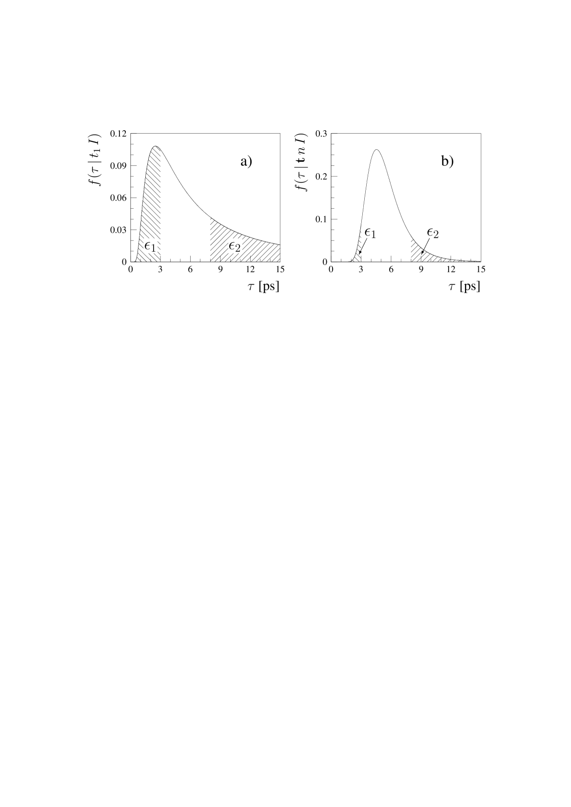
Figure 1: a) Unconstrained probability density function for $\tau$ based on a recorded decay time $t_{1}=5\;{\rm ps}$. The hatched areas represent integrals, $\epsilon_{1}=0.189$ and $\epsilon_{2}=0.465$, of the pdf in the intervals $(0,\tau_{a}=3\;{\rm ps})$ and $(\tau_{b}=8\;{\rm ps},\infty)$, respectively. b) Pdf for $\tau$ based on an average $\bar{t}=5\;{\rm ps}$ of $n=10$ recorded decay times with the integrals of the unconstrained pdf outside the allowed region for $\tau$ being reduced to $\epsilon_{1}=0.031$ and $\epsilon_{2}=0.102$.

That is, if the conditions (123) are fulfilled, normalization factors (121) and (122) are equal beyond the precision required for the particular inference. As admitted above, the invariance of the admissible parameter range, and consequently also the consistency of our reasoning, is not exact in such a case since for extremely large or extremely small values of measured decay times $t$ the equality (117) would not hold. But once $t_{1}$ has been recorded, it is very likely that the value of the inferred $\tau$ would also be of the same order of magnitude, i.e. it would be extremely unlikely for $\tau$ to be much smaller or much larger than $t_{1}$. Then, with $\tau\sim t_{1}$, it is also very unlikely that we would ever observe an event $t$ orders of magnitude different from $t_{1}$.

On the other hand, if the conditions (123) are not fulfilled (see, for example, Figure 1.a), our reasoning is clearly not consistent: by applying the two equally valid normalization factors, (121) and (122), we are able to arrive at significantly different probabilities for the same proposition, e.g. $P\bigl{(}a\tau\in(\tau_{1},\tau_{2})|at_{1}\,I\bigr{)}$, which is in direct contradiction with the consistency Desideratum III.a. The additional information that narrows the interval $(\tau_{a},\tau_{b})$ may still be very useful, but it is just that consistent probabilistic reasoning is impossible in such a situation.

In order to avoid such an inconsistency, we could have ignored the information, additional to $t_{1}$, and stretched $(\tau_{a},\tau_{b})$ to the whole positive half of the real axis. But this is not a solution either, since in this way we would have been arbitrarily ignoring some of the available information and basing our conclusions on what remains. Acting in explicit contradiction with Desideratum III.b, we would have allowed ideology to break into our inference, which is inadmissible for any scientifically respectable reasoning.

Thus, the only consistent solution to our problem of inference about the pre-constrained parameter $\tau$ would be provided by recording additional independent decay times,$t_{2},t_{3},...,t_{n}$, of particles of the same type. Then, the unconstrained probability distribution for $\tau$, based on the recorded data, is described by the following pdf:

$$f(\tau|t_{1}t_{2}...t_{n}I)=f(\tau|\mathbf{t}nI)=\frac{(n\bar{t})^{n}}{(n-1)!}\,\frac{1}{\tau^{n+1}}\,e^{-n\bar{t}/\tau}\ ,$$

where $\bar{t}$ is an average of the recorded decay times:

$$\bar{t}=\frac{1}{n}\,\sum_{i=1}^{n}t_{i}\ .$$

The distribution narrows as $n$ increases (see Figure 1.b). Therefore, by collecting enough data, the inconsistency is diminished beyond the required level: by diminishing the integrals $\epsilon_{1}$ and $\epsilon_{2}$ of the unconstrained pdf for $\tau$ outside the constrained domain, the limits $\tau_{a}$ and $\tau_{b}$ that caused the inconsistencies become irrelevant.

Our theory of consistent inference about parameters is therefore valid only if certain conditions are fulfilled, i.e. in the limit $\epsilon_{\pm}\to 0$. Such a theory is referred to as an effective theory, with the term coming from physics where all theories are effective. The precision of predictions of an effective theory is estimated by the proximity of the actual conditions to the ideal limit. The values of integrals $\epsilon_{\pm}$ (124), compared to zero, can thus serve as an estimate of the precision of our probabilistic inference about the pre-constrained parameters.

12 Calibration

The most striking achievement of the physical sciences is prediction.
Georg Pólya ([4], Chapter XIV, § 4, p. 64)

Thus far our theory of plausible inference about parameters has been developed by following Desiderata I.-III. only, while the implications of the operational Desideratum have not yet been considered. According to the latter Desideratum, in order to exceed the level of a mere speculation, our theory of inference about parameters must be exposed, i.e. must be able to make predictions that can be verified by experiments. The magnitudes considered by physicists such as mass, electric charge or reaction velocity have an operational definition: the physicist knows very well which operations he or she has to perform if he or she wishes to ascertain the magnitude of an electric charge, for example ([4], Chapter XV, § 4, p. 117). Is there a way for probability as a measure of a personal degree of belief to become operational, too?

Imagine we were given several numbers $x_{i}$, all produced by a random number generator according to a distribution $f(x_{i}|\theta_{i}I)$. While the form of the distribution is known to us, we do not know much about the values $\theta_{i}$ of the parameter: in general they can be different for each of the numbers $x_{i}$ generated and can be any number in the range $(\theta_{a},\theta_{b})$.

In fact, what we are asked for is to make probabilistic inferences about the unknown values $\theta_{i}$ on the basis of each datum $x_{i}$ separately. Based on our probability distribution for $\theta_{i}$, $p(\theta_{i}|x_{i}I)=f(\theta_{i}|x_{i}I)$, we should specify our confidence intervals $(\theta_{i,1},\theta_{i,2})$ such that

$$P\bigl{(}\theta_{i}\in(\theta_{i,1},\theta_{i,2})|x_{i}I\bigr{)}=\int_{\theta_{i,1}}^{\theta_{i,2}}f(\theta_{i}|x_{i}I)\,d\theta_{i}=\delta\ ,$$ (125)

with $\delta$ being the same for all inferences. Note that the interval for the inference of a particular value $\theta_{i}$ is not unique: it can be the shortest of all possible intervals, the central interval with $P(\theta_{i}\leq\theta_{i,1}|x_{i}I)=P(\theta_{i}>\theta_{i,2}|x_{i}I)=(1-\delta)/2$, the lower-most interval with $\theta_{i,1}=\theta_{a}$, the upper-most interval with $\theta_{i,2}=\theta_{b}$, or any other interval as long as the probability (125) equals $\delta$.

After the inference has been made, we learn the values $\theta_{i}$ of the parameter used in the random number generator. Then, our probability judgments are said to be calibrated if they agree with the actual frequencies of occurrence ([16], § 6.4, p. 142), i.e. if the fraction of inferences with the specified intervals containing the actual value of the parameter for the particular example, coincides with $\delta$.

The definition of long range relative frequency, although in some way less distinct than that of an electric charge, is still operational: it suggests definite operations that we can undertake to obtain an approximate numerical value of such a frequency ([4], Chapter XV, § 4,p. 117). Our theory thus cannot be expected to give a correct prediction each time, but it can be verifiable from its long range consequences, i.e. it can reasonably be expected to give the right answer in an assignable percentage of cases in the long run.

Under what conditions is a calibrated inference achieved? To answer this question we refer to the construction of classical confidence intervals (see [27], § 9.2.1, pp. 200-201 in [19], and Chapter 19 in [20]) and to fiducial theory (see refs. [25] and [20], § 19.44-19-47, pp. 156-162, § 26.26-26.29, pp. 440-442). Let $\alpha$ and $\alpha+\delta$ be probabilities for $x$ to take values less or equal to $x_{1}$ and $x_{2}$, respectively, given the value $\theta$ of the parameter of the (continuous) sampling distribution for $x$:

$$\begin{split}\alpha&=P\bigl{(}x\leq x_{1}(\theta)|\theta I\bigr{)}=F\bigl{(}x_{1}(\theta),\theta\bigr{)}\ ,\\ \alpha+\delta&=P\bigl{(}x\leq x_{2}(\theta)|\theta I\bigr{)}=F\bigl{(}x_{2}(\theta),\theta\bigr{)}\ .\end{split}$$ (126)

Then, the probability for $x$ to take a value in the interval $\bigl{(}x_{1}(\theta),x_{2}(\theta)\bigr{)}$, equals $\delta$:

$$P\bigl{(}x_{1}(\theta)\leq x<x_{2}(\theta)\bigr{)}=F\bigl{(}x_{2}(\theta),\theta\bigr{)}-F\bigl{(}x_{1}(\theta),\theta\bigr{)}=\delta\ ,$$ (127)

regardless of the value of $\alpha$. Let unique values $x_{1}(\theta)$ and $x_{2}(\theta)$, satisfying (126), exist for every $\theta$ in the range $(\theta_{a},\theta_{b})$, and for every $\alpha\in(0,1-\delta)$. It is easy to see that unconstrained location and scale parameters with $\mu\in(-\infty,\infty)$ and $\tau\in(0,\infty)$ meet such a requirement . The curves $x_{1}(\theta;\alpha)$ and $x_{2}(\theta;\alpha+\delta)$ are formed by varying $\theta$ in $x_{1}(\theta)$ and $x_{2}(\theta)$ but at fixed $\alpha$ and $\delta$ (see Figure 2) and the region between the two curves is known as a confidence belt.

Figure 2: Confidence belts in the case of distribution function $F(x,\theta)$ being a) strictly decreasing and b) strictly increasing in $\theta$.

Having the confidence belts defined, we return to the estimation of unknown values $\theta_{i}$ of the parameter. Given the measured value $x_{i}$, the required confidence interval $(\theta_{i,1},\theta_{i,2})$ is obtained by the intersection of the vertical line $x=x_{i}$ with the curves $x_{1}(\theta;\alpha)$ and $x_{2}(\theta;\alpha+\delta)$. By inspecting Figure 2 it becomes evident that the proposition

$$\theta_{i}\in(\theta_{i,1},\theta_{i,2})$$ (128)

is true if $x_{i}\in\bigl{(}x_{1}(\theta_{i}),x_{2}(\theta_{i})\bigr{)}$ and is wrong otherwise (see, for example, $\widetilde{x}_{i}$ and the corresponding confidence interval $(\widetilde{\theta}_{i,1},\widetilde{\theta}_{i,1})$ in Figure 2.b). This means that, according to (127), the probability for (128) to be true is exactly $\delta$ for every $\theta_{i}$, i.e. in the long run our inferences will be correct in $\delta$ per cent regardless the distribution of the values $\theta_{i}$.

In the case there exist unique values $\theta_{1,2}\in(\theta_{a},\theta_{b})$ for any $\alpha\in(0,1)$, any $\delta\in(0,1-\alpha)$ and for any $x_{1,2}\in(x_{a},x_{b})$, that solve equations (126), the cdf for $x$ is either strictly decreasing or strictly increasing in $\theta$. Then, by construction of confidence belts, the relations

$$\begin{split}F(x_{i},\theta_{i,1})&=\alpha+\delta\ ,\\ F(x_{i},\theta_{i,2})&=\alpha\ ,\end{split}$$

are always true for cdf’s strictly decreasing in $\theta$ (Figure 2.a), as is the case for functions with $\theta$ being a location or a scale parameter (see Section 4), while for strictly increasing distribution functions (Figure 2.b), the relations read:

$$\begin{split}F(x_{i},\theta_{i,1})&=\alpha\ ,\\ F(x_{i},\theta_{i,2})&=\alpha+\delta\ .\end{split}$$

Accordingly, the fraction $\delta$ of correct inferences can be expressed as:

$$\delta=\pm F(x_{i},\theta_{i,1})\mp F(x_{i},\theta_{i,2})=\pm F(x_{i},\theta_{i,1})\mp F(x_{i},\theta_{i,1}+\Delta\theta)\ ,$$ (129)

where the upper (lower) sign corresponds to cumulative distribution functions strictly decreasing (increasing) in $\theta$, while

$$\Delta\theta=\theta_{i,2}-\theta_{i,1}\ .$$

In the limit of infinitesimally small fractions $\delta$ and differences $\Delta\theta=d\theta$, equation (129) can be rewritten in terms of a differential of the distribution function with respect to $\theta$:

$$\delta=\mp\Bigl{(}\frac{\partial}{\partial\theta}F(x_{i},\theta)\Bigr{)}\,d\theta=\mp F_{2}(x_{i},\theta)\,d\theta\ .$$ (130)

But recall now our probabilistic inference about $\theta_{i}$: given the pdf $f(\theta|x_{i}I)$, the probability for $\theta_{i}$ being in the interval $(\theta,\theta+d\theta)$ reads:

$$p(\theta|x_{i}I)=f(\theta|x_{i}I)\,d\theta\ .$$

Thus, we finally came to the point when we are able to answer: our inference will be calibrated, i.e. the assigned probability will coincide with the fraction $\delta$ of confidence intervals containing the true values of the parameter, if and only if

$$f(\theta|x_{i}I)=\mp F_{2}(x_{i},\theta)\ .$$ (131)

For location parameters with the cumulative distribution function (35) for the sampling variable $x$, the condition (131) implies the calibrated pdf for $\theta$ be:

$$f(\mu|x_{i}I)=-\frac{\partial}{\partial\mu}\int_{-\infty}^{x_{i}-\mu}\phi(u)\,du=\phi(x_{i}-\mu)=f(x_{i}|\mu I)\ .$$

The above pdf for $\theta$ coincides with the one obtained by following the basic Desiderata of consistent inference, implying the consistency factor $\pi(\mu)$ to be constant (10). Therefore, the only consistent way of inference about location parameters is also the only one that is calibrated.

The latter is also true for inferences about scale parameters with the appropriate distribution function (39). Namely,

$$f(\tau|t_{i}I)=-\frac{\partial}{\partial\tau}\int_{0}^{\frac{t_{i}}{\tau}}\phi(u)\,du=\frac{t_{i}}{\tau^{2}}\,\phi\Bigl{(}\frac{t_{i}}{\tau}\Bigr{)}=\frac{t_{i}}{\tau}\,f(t_{i}|\tau I)$$

corresponds to $\pi(\tau)=\tau^{-1}$ as already determined in (10).

The probability distributions for location, scale or dispersion parameters that were assigned in consistent way, passed an important test: they are all calibrated. The question can be raised whether there are any other types of parameters that are also in accordance with the calibration requirement (131)? We restrict the answer only to parameters whose pdf can be written in the form of the Consistency Theorem (64), obtained by requiring logically independent pieces of information to be commutative. By combining the two equations we obtain:

$$\pi(\theta)\,F_{1}(x,\theta)\pm\eta(x)\,F_{2}(x,\theta)=0\ ,$$ (132)

where the upper (lower) sign stands for cdf’s which are strictly decreasing (increasing) in $\theta$. By defining function $G(x,\theta)$ as a difference (sum),

$$G(x,\theta)\equiv h(x)\mp k(\theta)\ ,$$

with $h(x)$ and $k(\theta)$ being related to $\pi(\theta)$ and $\eta(x_{1})$ as

$$h^{\prime}(x)=\eta(x)\ \ \text{and}\ \ k^{\prime}(\theta)=\pi(\theta)\ ,$$

equation (132) can be rewritten as

$$F_{1}(x,\theta)\,G_{2}(x,\theta)-F_{2}(x,\theta)\,G_{1}(x,\theta)=0\ ,$$

with $G_{1}(x,\theta)=\eta(x)$ and $G_{2}(x,\theta)=\pi(\theta)$ being strictly positive functions (see Section 6). But as we saw in Section 5, the general solution of such a differential functional equation is a distribution function $F(x,\theta)$ of the form

$$F(x,\theta)=\Phi(z-\mu)\ ,$$

where

$$z\equiv h(x)\ \ \text{and}\ \ \mu\equiv\pm k(\theta)\ ,$$

i.e. a distribution function that corresponds to $\mu$ being a location parameter (35). Therefore, in the limit of complete prior ignorance, an inference about a parameter $\theta$ that is subject to the calibration condition (131), is necessarily reducible to an inference about a location parameter. Note that this result was first obtained by Dennis Lindley [28] by combining the calibration condition (131) and the Bayes’ theorem with a prior pdf $f(\theta|I)$ which is independent of data $x$.

It is interesting to note that the above result is identical to the result obtained at the end of Section 5 and discussed in Section 7, despite the fact that the requirements of logical consistency and that of calibration may appear, at least at first sight, as almost diametrically opposed starting points. As a very important consequence, every probabilistic inference about a parameter of a sampling distribution that we are sure is consistent will thus at the same time also be calibrated and, vice versa, every calibrated inference, based on a posterior probability distribution that is factorized according to the Consistency Theorem, will simultaneously be logically consistent, too.

Recall Section 2 where we chose a set of functions, called probabilities, out of all possible plausibility functions, suitable for representing our degree of belief according to the basic Desiderata. The main reason for such a choice was that for the probabilities the basic equations for manipulating plausibilities - the product and the sum rule, (1) and (2)- are of especially simple forms. But now we realize another advantage of probabilities over other plausibility functions: it is only for probabilities that the assigned degrees of belief exactly coincide with the long term relative frequencies. Other plausibilities are one-to-one functions of probabilities, so their values correspond to (the same) one-to-one functions of the relative frequencies. Again, this does not imply that predictions in terms of probabilities are more reliable than predictions in terms of any other set of plausibility functions: they are just the easiest to interpret.

The predictions of the systems of plausible reasoning, however, that are not isomorphisms of the probability system, are, apart from being inconsistent, also necessarily uncalibrated. This means that in general their predictions in terms of long-range frequencies are not correct.

Take, as an example, the power-law distribution with the pdf
$$f(x|\theta I)=(\theta+1)\,x^{\theta}\ ,$$ (133)
the ranges of $x$ and $\theta$
$$x\in(0,1)\ \ \text{and}\ \ \theta\in(-1,\infty)\ ,$$ (134)
and the corresponding cdf

$$F(x,\theta)=\int_{0}^{x}(1+\theta)\,x^{\prime\,\theta}\,dx^{\prime}=x^{\theta+1}\ .$$

Due to the range of $x$, the cdf is strictly decreasing in $\theta$, therefore the calibration condition for the inference about the parameter reads:
$$f(\theta|xI)=-F_{2}(x,\theta)=(\theta+1)\,x^{\theta}\;\frac{(-x\ln{x})}{\theta+1}\ .$$ (135)
The ratio of the pdf’s for $\theta$ and $x$, (133) and (135),

$$\frac{f(\theta|xI)}{f(x|\theta I)}=\frac{-x\ln{x}}{\theta+1}\ ,$$

implies consistency and normalization factors of the form

$$\pi(\theta)=\frac{1}{\theta+1}$$

and

$$\eta(x)=-\frac{1}{x\ln{x}}\ .$$

Their integrals,

$$z\equiv h(x)=\int\eta(x)\,dx=-\ln{(-\ln{x})}$$

and

$$\mu\equiv k(\theta)=\int\pi(\theta)\,d\theta=\ln{(1+\theta)}\ ,$$

with the domains of both being the complete real axis (c.f. equation (134)),

$$z,\mu\in(-\infty,\infty)\ ,$$

allow for a reduction of the inference about parameter $\theta$ to an inference about a location parameter $\mu$ of the sampling distribution of the variate $z$ with the corresponding cdf:

$$F(z,\mu)=\Phi\bigl{(}-\ln{(-\ln{x})}-\ln{(1+\theta)}\bigr{)}=\Phi(z-\mu)\ .$$

Indeed:

$$f(z|\mu I)=f\bigl{(}x(z)|\theta(\mu)I\bigr{)}\,\Bigl{|}\frac{dx}{dz}\Bigr{|}=e^{-(z-\mu)}\exp{\bigl{\{}-e^{-(z-\mu)}\bigr{\}}}\ .$$

As a counter-example, i.e. as an example with the cdf of the sampling distribution being neither strictly increasing nor decreasing with respect to all of its parameters, we refer to the Weibull distribution ([12], § 5.33, pp. 189-190) with the pdf of the form:

$$f(t|\theta\,\tau I)=\frac{\theta}{\tau}\Bigl{(}\frac{t}{\tau}\Bigr{)}^{\theta-1}\exp{\biggl{\{}-\Bigl{(}\frac{t}{\tau}\Bigr{)}^{\theta}\biggr{\}}}\ .$$

The range of the variate $t$, as well as the ranges of both parameters $\theta$ and $\tau$, coincide with the positive half of the real axis:

$$t,\tau,\theta\in(0,\infty)\ .$$

Let the value of the scale parameter $\tau$ of the distribution be known and let $x$ be a normalized variate:

$$x=\frac{t}{\tau}\ \ ,\ \ x\in(0,\infty)\ ,$$

with the appropriate pdf,
$$f(x|\theta I)=f\bigl{(}t(x)|\theta\,\tau I\bigr{)}\,\Bigl{|}\frac{dt}{dx}\Bigr{|}=\theta x^{\theta-1}\exp\bigl{(}-x^{\theta}\bigr{)}\ ,$$ (136)
and cdf:

$$F(x,\theta)=1-\exp\bigl{(}-x^{\theta}\bigr{)}\ .$$

Clearly, the cdf is decreasing in $\theta$ for $x<1$, but increasing in $\theta$ for $x>1$.

13 Reduction to inference about location parameters under more general conditions

We can provide a consistent and calibrated parameter inference only when the problem is reducible to estimation of a location parameter. But, as we saw in the case of the Weibull distribution, reduction to a location parameter estimation is not always possible. Nevertheless, under very general conditions, there is a neat way out of such difficult situations.

When lacking any additional prior knowledge, all information about an inferred parameter $\theta$ of a specified sampling distribution that can be extracted from the measured events, is contained in the value of the likelihood. After collecting $n$ independent events $x_{i}$, the likelihood density for $\mathbf{x}$ reads:

$$f\bigl{(}\mathbf{x}=(x_{1},x_{2},...,x_{n})|\theta I)=\prod_{i=1}^{n}f(x_{i}|\theta I)\ .$$

Let $\hat{\theta}$ be the value of the parameter that maximizes the value of the likelihood density, given a particular set of collected events $\mathbf{x}$:

$$\hat{\theta}=\hat{\theta}(x_{1},x_{2},...,x_{n})=\hat{\theta}(\mathbf{x})\ \ \ :\ \ \ f(\mathbf{x}|\theta I)\big{|}_{\theta=\hat{\theta}}=\text{max.}$$

Suppose also that the integral

$$R^{2}(\theta)=\int\limits_{x}\Bigl{(}\frac{\partial}{\partial\theta}\ln{f(x^{\prime}|\theta I)}\Bigr{)}^{2}f(x^{\prime}|\theta I)\,dx^{\prime}$$

exists for every $\theta$ in its permissible range. Then, as the number $n$ of measurements $x_{i}$ increases, the sampling distribution for $\hat{\theta}(\mathbf{x})$ converges to a Gaussian distribution with $\mu=\theta$ and $\sigma(\theta)=\bigl{(}R(\theta)\sqrt{n}\bigr{)}^{-1}$ (see, for example, [20], § 18.10, pp. 52-53 and § 18.16, pp. 57-58). The width of the distribution decreases with increasing $n$. For a sufficiently large number of measurements the width can be approximated by $\sigma(\theta)\simeq\sigma(\hat{\theta})$,

$$\sigma(\hat{\theta})=\frac{1}{R(\hat{\theta})\sqrt{n}}\ ,$$

leaving $\theta$ as a pure location parameter of the distribution for $\hat{\theta}(\mathbf{x})$,

$$f(\hat{\theta}|\theta I)=\frac{1}{\sqrt{2\pi}\sigma(\hat{\theta})}\exp{\Biggl{\{}-\frac{(\hat{\theta}-\theta)^{2}}{2\sigma^{2}(\hat{\theta})}\Biggr{\}}}\ ,$$

thus allowing to make a consistent inference about $\theta$. The required number of collected events depends on the precision required for the inference about the parameter and on the form of the sampling distribution (see Figure 3 with two examples for the Weibull distribution).

Figure 3: Sampling distribution for $\hat{\theta}(\mathbf{x})$ resulting from maximizations of the likelihood density $f(\mathbf{x}|\theta I)=\prod_{i=1}^{n}f(x_{i}|\theta I)$ that is a product of Weibull pdf’s (136) (continuous line) and the limiting Gaussian or normal distribution $N\bigl{(}\mu=\theta,\sigma=(R(\theta)\sqrt{n})^{-1}\bigr{)}$ (dashed line) for $\theta=5$ and for $n$ being a) 5 and b) 100.

14 Inferring parameters of counting experiments

Let an urn contain balls that are identical in every respect except that some of the balls are coloured white and the remaining ones are coloured red. Such an urn is usually referred to as the Bernoulli urn and drawing from the urn is referred to as a Bernoulli trial. We draw a ball from the urn blindfolded, observe and record its colour, put it back into the urn and thoroughly shake the urn in order to minimize any possible correlations between successive draws. Then we repeat the process until $n_{0}$ balls have been drawn, out of which $n$ have been recorded to be white ($0\leq n\leq n_{0}$). If correlations between the draws can be neglected, the probability of recording $n$ white balls in $n_{0}$ draws is given by the binomial distribution ([12], § 5.2-5.7, pp. 163-168):

$$p(n|\theta n_{0}I)={n_{0}\choose n}\,\theta^{n}\,(1-\theta)^{n_{0}-n}\ ,$$

where the parameter $\theta$ of the distribution coincides with the fraction of the white balls in the urn.

On the basis of known $n$ and $n_{0}$ we would like to make a probabilistic inference about the value of the parameter $\theta$. Lacking any additional prior information, we write the pdf for $\theta$ in accordance with (63):

$$f(\theta|nn_{0}I)=\frac{\pi(\theta)\,p(n|\theta n_{0}I)}{\int_{0}^{1}\pi(\theta^{\prime})\,p(n|\theta^{\prime}n_{0}I)\,d\theta^{\prime}}=\frac{\pi(\theta)}{\eta(n,n_{0})}\,p(n|\theta n_{0}I)\ ,$$

where the form of the consistency factor $\pi(\theta)$ is yet to be determined.

We showed that we are able to uniquely determine the form of a consistency factor only in presence of invariance of the sampling distribution under a continuous (Lie) group of transformations. But in the case of counting experiments, with a discrete variate $n$ of the sampling distribution, such an invariance is evidently absent. In this way we loose ground to uniquely determine the form of the consistency factor simply by following Cox-Pólya-Jaynes Desiderata. If we insist on making a ’probabilistic’ inference, we are therefore restricted to using ’consistency factors’, also referred to as non-informative priors, whose forms are chosen on the basis of some ad hoc criteria. But no matter how carefully these criteria and non-informative priors are specified, there is no guarantee that in this way our reasoning remains consistent. Then, without being protected by the Desiderata, we stand at the mercy of all kinds of paradoxes, stemming from inconsistencies that we may unintentionally have committed.

As an example, imagine a large number of urns, each containing an unknown fraction of white balls. We make a series of Bernoulli trials by drawing a single ball from each of the urns, i.e. $n_{0}=1$ for each of the draws. The outcome of drawing from the $i$-th urn can be a white ($n=1$) or a red ($n=0$) ball and the corresponding likelihood reads:

$$p(n|n_{0}\theta_{i}I)=\begin{cases}\ \ \ \ \theta_{i}\ \ \ \ \,;\ \ n=1\\ 1-\theta_{i}\ \ ;\ \ n=0\end{cases}\ ,$$

where $\theta_{i}$ is the (unknown) fraction of white balls in the $i$-th urn. Let us try to make a ’probabilistic’ inference about the parameter by using a uniform non-informative prior distribution of ’probability’ for $\theta_{i}$:

$$\text{'}f(\theta|I)\text{'}=1\ .$$

Then, a ’pdf’ can be assigned to $\theta_{i}$ simply by using Bayes’ theorem (25):

$$\text{'}f(\theta_{i}|nn_{0}I)\text{'}=\frac{\text{'}f(\theta_{i}|I)\text{'}\,p(n|n_{0}\theta_{i}I)}{\int_{0}^{1}\text{'}f(\theta_{i}|I)\text{'}\,p(n|n_{0}\theta_{i}I)\,d\theta_{i}}=\begin{cases}\ \ \ \ \ 2\theta_{i}\ \ \ \ \ \ \,;\ \ n=1\\ 2(1-\theta_{i})\ \ ;\ \ n=0\end{cases}\ .$$ (137)

If (137) is truly a pdf for $\theta$, then a ’probability’

$$\text{'}P\bigl{(}\theta_{i}\in(\theta_{1},\theta_{2})|nn_{0}I)\text{'}=\int_{\theta_{1}}^{\theta_{2}}\text{'}f(\theta_{i}|nn_{0}I)\text{'}\,d\theta_{i}$$

should cover the true value of $\theta_{i}$ in $100\,\text{'}P\bigl{(}\theta_{i}\in(\theta_{1},\theta_{2})|nn_{0}I)\text{'}$ per cent of the inferences, but it is easy to see that such an inference is in general not calibrated. Let us choose the shortest intervals with the ’probability’ of containing $\theta_{i}$ being 50% (see Figure 4):

$$(\theta_{1},\theta_{2})=\begin{cases}\ \ \ \bigl{(}\frac{\sqrt{2}}{2},1\bigr{)}\ \ \ \ \ \,;\ \ n=1\\ \bigl{(}0,1-\frac{\sqrt{2}}{2}\bigr{)}\ \ ;\ \ n=0\end{cases}\ .$$

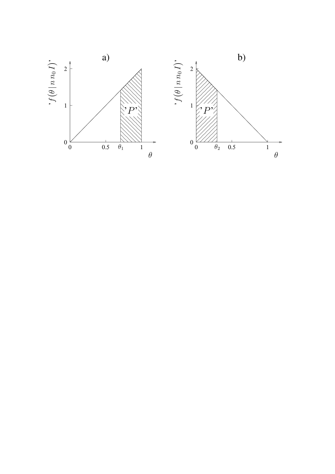
Figure 4: ’Probability density functions’ assigned to the parameter of a binomial distribution when the number of draws is $n_{0}=1$ and the result of drawing is either a) favourable ($n=1$) or b) non-favourable ($n=0$). The distributions are assigned by choosing a uniform non-informative prior. The integrals of the ’densities’, ’probabilities’ ’$P$’ (hatched regions), on the intervals a) $(\theta_{1}=\sqrt{2}/2,\theta_{2}=1)$ and b) $(\theta_{1}=0,\theta_{2}=1-\sqrt{2}/2)$ amount to 0.5

If, for example, the fraction of white balls in each of the urns were exactly one-half, our intervals would never cover the true value, i.e. our inference is manifestly non-calibrated. Non-informative priors of different forms, for example

$$\text{'}f(\theta|I)\text{'}=\frac{1}{\theta(1-\theta)}\ \ \text{or}\ \ \text{'}f(\theta|I)\text{'}=\frac{1}{\sqrt{\theta(1-\theta)}}$$

(see [2], § 12.4.3, p. 384, eq. (12.50), and [18], § 11.3, p. 106, eq. (11.63)), are not immune to such kind of problems, either.

As on two previous occasions, such an obstacle in the way of consistent parameter inference can be overcome simply by collecting more data, such that

$$\begin{split}n_{0}-n&\gg 1\ ,\\ n&\gg 1\ .\end{split}$$ (138)

When the above condition is fulfilled, the sampling distribution for $x_{n}$,

$$x_{n}\equiv\frac{n}{n_{0}}\ ,$$

converges to a Gaussian distribution $N(\mu,\sigma)$ ([12], § 4.15, pp. 138-140) with

$$\mu(\theta)=\theta\ \ \text{and}\ \ \sigma(\theta)=\sqrt{\frac{\theta(1-\theta)}{n_{0}}}$$

in the sense that

$$\begin{split}\sum_{n=n_{1}}^{n_{2}}p(n|n_{0}\theta I)&=\sum_{n=n_{1}}^{n_{2}}p(x_{n}|n_{0}\theta I)\\ \simeq\int_{x_{n_{1}}-\frac{1}{2n_{0}}}^{x_{n_{2}}+\frac{1}{2n_{0}}}f(x|\mu\sigma I)\,dx&=\int_{x_{n_{1}}-\frac{1}{2n_{0}}}^{x_{n_{2}}+\frac{1}{2n_{0}}}\frac{1}{\sqrt{2\pi\sigma}}\,\exp\biggl{\{}-\frac{(x-\mu)^{2}}{2\sigma^{2}}\biggr{\}}\,dx\ .\end{split}$$

The dispersion parameter $\sigma(\theta)$ of the limiting distribution decreases with increasing number of draws from the urn and for sufficiently large $n_{0}$ it can be approximated by

$$\sigma(\theta)\simeq\sigma(x_{n})=\sqrt{\frac{x_{n}(1-x_{n})}{n_{0}}}\ .$$

In this way, $\theta$ becomes a pure location parameter of a Gaussian distribution with the corresponding uniform consistency factor and with the corresponding pdf:

$$f(\theta|x_{n}n_{0}I)=\frac{\pi(\theta)}{\eta(x_{n})}\,p(x_{n}|n_{0}\theta I)=\frac{1}{\sqrt{2\pi}\sigma(x_{n})}\,\exp\biggl{\{}-\frac{(x_{n}-\theta)^{2}}{2\sigma^{2}(x_{n})}\biggr{\}}\ .$$

At this point we find it appropriate, for the sake of completeness, to make a comment on the density of information $nn_{0}I$ that probability $p(\theta|nn_{0}I)$ is conditional upon. Recall that a continuity requirement concerning sets of different states of knowledge about inferred propositions was listed within the common sense Desideratum II. But with $I$ merely representing information about the type of counting sampling distribution, and with $n_{0}=1$ being a fixed number of experiments performed, the possible information about $\theta$ after the first trial consists two atoms, $n=0$ and $n=1$, that do not allow for such a requirement to be met. In this way the proof of Cox’s Theorem (see, for example, [10], or [2], § 2.1-2.2, pp. 24-45), stating that the basic Desiderata necessarily imply (up to an isomorphic transformation) the product rule (1), the sum rule (2), and their corollary, Bayes’ Theorem (25), misses an indispensable fact. That is, in a situation like that there is no explicit reason why an inference about a parameter of a sampling distribution should be made in accordance with the Consistency Theorem that is deduced by assuming, among other things, Bayes’ Theorem to be the only consistent way to update the probability distribution for the inferred parameter (recall Section 6). However, in the dense limit (138), the continuity of information (i.e. of $n/n_{0}$) is recovered and the procedure of inference about $\theta$ becomes uniquely determined by the adopted Desiderata.

Note that for a consistent and calibrated inference both conditions of (138) must be met. Suppose for a moment that only

$$n_{0}-n\gg 1$$

holds so that the binomial sampling distribution can be approximated by the Poisson limit ([12], § 5.8-5.9, pp. 168-171):

$$p(n|\mu I)=\frac{\mu^{n}}{n!}\,e^{-\mu}\ ,$$

where the parameter $\mu$ of the distribution represents the expected number of white balls drawn. Suppose that only red balls are drawn, i.e. $n=0$, and that we want to make a ’probabilistic’ inference about $\mu$ by choosing a uniform non-informative prior. The corresponding ’pdf’ for $\mu$ then reads:

$$\text{'}f(\mu|n=0\,I)\text{'}=\frac{\text{'}f(\mu|I)\text{'}\,p(n=0|\mu I)}{\int_{0}^{\infty}\text{'}f(\mu^{\prime}|I)\text{'}\,p(n=0|\mu^{\prime}I)\,d\mu^{\prime}}=e^{-\mu}\ ,$$

which implies a ’probability’ for $\mu\leq\mu_{0}$,

$$\text{'}P(\mu\leq\mu_{0}|nI)\text{'}=\int_{0}^{\mu_{0}}\text{'}f(\mu|n=0\,I)\text{'}\,d\mu=1-e^{-\mu_{0}}\ ,$$

or, equivalently, implies a ’probability’ for $\mu>\mu_{0}$,

$$\text{'}P(\mu>\mu_{0}|nI)\text{'}=\int_{\mu_{0}}^{\infty}\text{'}f(\mu|n=0\,I)\text{'}\,d\mu=e^{-\mu_{0}}\ ,$$

where $\mu_{0}$ takes an arbitrary positive value. For example, for $\mu_{0}=3$, the two ’probabilities’ equal $\sim 0.95$ and $\sim 0.05$, respectively.

Imagine now such draws from a number of urns $N$, all ending up with $n_{i}=0$. We can make use of the general sum rule (3) and calculate a ’probability’, $\text{'}P_{N}\text{'}$, for at least one out of $N$ parameters $\mu_{i}$ being greater than $\mu_{0}$. Since the draws from different urns are not correlated, the ’probability’ equals:

$$\text{'}P_{N}\text{'}=1-\Bigl{(}1-\,\text{'}P(\mu>\mu_{0}|nI)\text{'}\Bigr{)}^{N}\ .$$

With increasing $N$, the value of $\text{'}P_{N}\text{'}$ approaches unity: for a sufficiently large number of urns we can claim with ’certainty’ that at least for one of the urns the parameter $\mu_{i}$ is greater than $\mu_{0}$, regardless of the chosen value of the latter. But claiming the existence of white balls in the urns on the basis of observing only red ones, is clearly a logically unacceptable result, pointing to serious flaws of this kind of inference. Note that it was not the choice of the uniform non-informative prior that was decisive for the above result since every $\text{'}f(\mu|I)\text{'}$ with the existing integral

$$\int_{0}^{\infty}\text{'}f(\mu^{\prime}|I)\text{'}\,p(n=0|\mu^{\prime}I)\,d\mu^{\prime}$$

would lead to the same kind of a logically unacceptable conclusion.

If an urn contains only red balls, the requirement

$$n\gg 1$$

can never be met. Is there some kind of inference that could be made in such cases? Let us perform two Bernoulli trials by drawing $n_{0}$ and $2n_{0}$ balls from an urn, with all of the drawn balls in both trials being red. The evidence against the presence of white balls in the urn that was obtained by the second trial may be reasonably held to be stronger than the evidence from the first trial. Yet how much stronger? It seems to us that in such cases the degrees of belief, although still comparable, cannot be expressed quantitatively (see also [4], Chapter XV, p. 137), i.e. in order to avoid all sorts of paradoxes we should remain on a qualitative level.

15 Historical digression

In Section 6 we stressed that, contrary to the prior probability distribution in Bayes’ Theorem (25 – 26), the consistency factor in equations (63 – 66) does not represent any kind of probability distribution. Overlooking this fact led to perpetual philosophical argument throughout the history of probabilistic reasoning, with far-reaching practical consequences.

A natural starting point for every sequential updating of information is a state of complete ignorance, e.g. complete prior ignorance about the value of an inferred parameter $\theta$ of a sampling distribution for $x$. The original sin is then committed in an attempt to make use of Bayes’ Theorem, (25) or (26), in such a situation. According to the Theorem, in order to obtain a probability distribution for the inferred parameter after observing $x_{1}$ both the likelihood, i.e. the probability for observing $x_{1}$ given a particular value of the parameter, and a prior probability distribution for $\theta$, i.e. a distribution of our belief in different values of the parameter prior to observing $x_{1}$, must be provided. With the known form of the sampling distribution, the calculation of the likelihood is a rather straightforward task. The problem arises when we try to formulate the distribution of our belief prior to the first recorded event, for up untill then we had been completely ignorant about the possible values of $\theta$. What we are trying to do is to assign a prior probability distribution based on ignorance, i.e. we are trying to establish the so-called ignorance or non-informative probability distributions. But according to the definition of probability adopted as a degree of reasonable belief that is based on relevant information at hand (see Section 2), a probability assigned on grounds of ignorance is simply a contradiction in terms. A prior probability distribution that is based only on ignorance thus cannot be the realm of a consistent probability theory. We will see that apart from being self-contradicting on the conceptual level, the concept of ignorance or non-informative priors inevitably also produces many practical inconsistencies and paradoxes.

This delusion about probability distributions based on ignorance has been present for more than two centuries. In a scholium to his essay [13] Bayes suggested that in the absence of all prior knowledge it is reasonable to assume a uniform distribution for $p$, where $p$ stands for, for example, an unknown fraction of white balls in an urn experiment as described in Section 14. Laplace ([5], p. XVII) was also very explicit on the same subject:“When the probability of a single event is unknown we may suppose it equal to any value from zero to unity.” The above assumption is usually referred to as the Bayes principle ([12], § 8.19, p. 298), the Laplace principle of insufficient reason [31] or the principle of indifference ([2], § 2.4, p. 40). When applied to estimation of a general unknown parameter, the assumption would read: in the limit of complete prior ignorance about the value of an inferred parameter, the prior distribution should be uniform.

We strongly disagree with such a rule and propose a very simple rule to replace it: when there is no (prior) information, no (prior) probabilities are to be assigned whatsoever. Or to paraphrase de Finetti: prior probability does not exist. Knowing that a uniform prior probability distribution in the range $(\theta_{a},\theta_{b})$ has been assigned to the value of a parameter $\theta$ as a result of positive knowledge, and not knowing anything about $\theta$ with the exception of its admissible range, are two fundamentally different states of knowledge.

In order to illustrate the difference, we return to drawing coloured balls from urns. Imagine having a good number of urns, each containing red and white balls, with the fractions of white balls, $\theta_{i}$, in each of the urns being unknown. According to the first scenario, we possess information that the fractions are distributed uniformly in the range (0,1), while according to the second scenario we know nothing about the distribution of the values of $\theta_{i}$. It is easy to see that the two states of knowledge are completely different.

In the first case it is possible to assign a probability for $\theta_{i}$ of the $i$-th urn which is in an arbitrary interval $(\theta_{1},\theta_{2})\subset[0,1]$ even before drawing the first ball from the urn simply by integrating the (uniform) prior probability distribution:

$$P\bigl{(}\theta_{i}\in(\theta_{1},\theta_{2})|I\bigr{)}=\int_{\theta_{1}}^{\theta_{2}}f(\theta|I)\,d\theta=\int_{\theta_{1}}^{\theta_{2}}d\theta=\theta_{2}-\theta_{1}\ .$$ (139)

On making the first draw from the $i$-th urn, it can be either a white ($n_{i}=1$) or a red ($n_{i}=0$), implying the corresponding likelihood to be:

$$p(n_{i}|\theta_{i}I)=\begin{cases}\ \ \ \ \ \theta_{i}\ \ \ \ \ \,\ ;\ \ n_{i}=1\\ (1-\theta_{i})\ \ ;\ \ n_{i}=0\ ,\end{cases}$$

The updated posterior probability therefore reads:

$$P\bigl{(}\theta_{i}\in(\theta_{1},\theta_{2})|n_{i}I\bigr{)}=\begin{cases}\ \ \ \ \ \ \ \ \ \ \ \,\theta_{2}^{2}-\theta_{1}^{2}\ \ \ \ \ \ \ \ \ \ \ \ \ ;\ \ n_{i}=1\\ (1-\theta_{1})^{2}-(1-\theta_{2})^{2}\ \ ;\ \ n_{i}=0\ ,\end{cases}$$ (140)

where the update was made by using Bayes’ Theorem (25). Note that both probabilities are calibrated: when repeating the above assessments for all of the urns, intervals $(\theta_{1},\theta_{2})$ contain the true fractions of white balls in the each of the urns in $100P\bigl{(}\theta_{i}\in(\theta_{1},\theta_{2})|I\bigr{)}$ percent of cases before any of the balls were drawn, while after drawing the coverage is exactly $P\bigl{(}\theta_{i}\in(\theta_{1},\theta_{2})|n_{i}I\bigr{)}$.

Within the second scenario, with complete prior ignorance about the distribution of $\theta_{i}$ within the urns, we cannot make a probabilistic inference about fraction of white balls in a particular urn before any of the balls is drawn. The statement that the probability for $\theta_{i}$ to be in the interval $(\theta_{1},\theta_{2})$ equals the length of the interval (see eq. (139)) would in general be uncalibrated unless the distribution of $\theta_{i}$ within the urns is truly uniform - but this we do not know and need not be true. The same holds for the probability statement (140) after drawing one ball from each of the urns. We saw in the previous section that in the limit of complete prior ignorance, consistent and calibrated probability statements about the parameters $\theta$ can be made only after drawing enough balls from each of the urns so that the Gaussian limit of the binomial sampling distribution can be applied.

Many failed to recognize the fundamental difference between knowing the prior probability distribution of an inferred parameter to be uniform and not knowing anything about the value of the parameter. Harold Jeffreys, for example, wrote ([15], § 1.22, p. 29): “If there is originally no ground to believe one of a set of alternatives rather than another, their prior probabilities are equal.” The same standpoint was persistently advocated also by Edwin Jaynes ([2], § 18.11.1, p. 573): “Before we can use the principle of indifference to assign numerical values of probabilities, there are two different conditions that must be satisfied: (1) we must be able to analyze the situation into mutually exclusive, exhaustive possibilities; (2) having done this, we must then find available information gives us no reason to prefer any of the possibilities to any other. In practice, these conditions are hardly ever met unless there is some evident element of symmetry in the problem. But there are two entirely different ways in which condition (2) might be satisfied. It might be satisfied as a result of ignorance, or it might be satisfied as a result of positive knowledge about the situation.”

We could not agree more with Jaynes if it were not for the last sentence. Take, for example, two different samples of radionuclides. For the first sample we do not know anything about the isotopes except that the permissible range of their expected decay times is in an interval $(\tau_{a},\tau_{b})$, while for the second sample the isotopes were chosen in such a way that the distribution of their expected decay times can be well approximated by a uniform distribution in the same interval. As a result of ignorance, we cannot make inferences about the expected decay times $\tau_{i}$ of the isotopes in the first sample before measuring their actual decay times $t_{i}$. After the decay time $t_{i}$ of the $i$-th isotope is measured, however, we can make a probabilistic statement about $\tau_{i}$ according to (64):

$$f(\tau_{i}|t_{i}I)=\frac{\pi(\tau_{i})}{\eta(t_{i})}\,f(t_{i}|\tau_{i}I)=\frac{t_{i}}{\tau_{i}}\,f(t_{i}|\tau_{i}I)=\frac{t_{i}}{\tau^{2}_{i}}\,e^{-t_{i}/\tau_{i}}\ ,$$

where $I$ stands for prior ignorance about the expected decay time of a particular radionuclide, while the consistency factor $\pi(\tau_{i})$ was chosen according (10). From Section 11 we recall that our inference is consistent if the integral of the above pdf outside the admissible range for $\tau_{i}$ is small compared to the precision required. For the second sample of isotopes, as a result of positive knowledge, there is a pdf for the expected decay time of each of the isotopes at our disposal even prior to measuring the actual decay times:

$$f(\tau_{i}|I^{\prime})=\begin{cases}(\tau_{b}-\tau_{a})^{-1}\ \ ;\ \ \tau_{a}<\tau_{i}<\tau_{b}\\ \ \ \ \ \ \ \ 0\ \ \ \ \ \ \ \ \ \,\,\ ;\ \ \text{otherwise}\ \ ,\end{cases}$$

where $I^{\prime}$ stands for positive prior knowledge. After $t_{i}$ is measured (and not knowing the results of other possible measurements of decay times from the same sample), the distribution of our belief can be updated by means of Bayes’ theorem (29):

$$f(\tau_{i}|t_{i}I^{\prime})=\frac{f(\tau_{i}|I^{\prime})\,f(t_{i}|\tau_{i}I^{\prime})}{\int_{\tau_{a}}^{\tau_{b}}f(\tau^{\prime}_{i}|I^{\prime})\,f(t_{i}|\tau^{\prime}_{i}I^{\prime})\,d\tau^{\prime}_{i}}\ .$$

Note that when appropriate prior pdf’s exist, the inferences are always consistent and calibrated. Figure 5 shows examples of inferences with and without existing prior probability distributions.

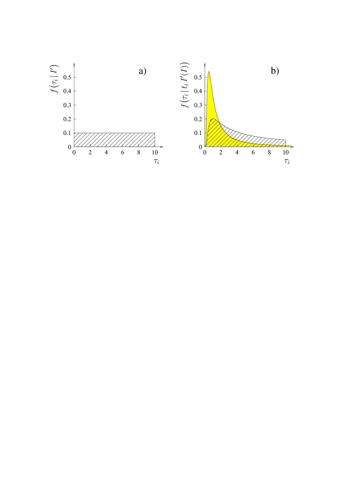
Figure 5: Probability density functions for the expected decay time $\tau_{i}$ of the $i$-th isotope from a sample of isotopes with the expected decay times distributed approximately uniformly in an admissible range $(\tau_{a},\tau_{b})=(0,10)$ (hatched areas), and the corresponding pdf for an isotope from a sample with the expected decay times in the same interval but with an unknown distribution of their actual values (shaded area). Figure a) displays the pdf before any of the actual decay times are measured, while Figure b) shows appropriate pdf’s based on a measured value $t_{i}=1$ in both cases. All decay times are given in arbitrary but equal units. While the hatched histograms are limited within the permissible range, the integral of the shaded pdf in the range $(10,\infty)$ is approximately $\epsilon_{2}=0.095$.

Apart from the problems with calibration, the Bayes postulate contains also some insurmountable inconsistencies. Suppose we are estimating a parameter $\theta$ with no prior information available. According to the postulate, the prior ’probability’ distribution in such a case is given by a uniform ’pdf’:

$$\text{'}f(\theta|I)\text{'}=1.$$

But, instead of $\theta$, we could have equally well chosen different parameterization, say $\lambda(\theta)$, where

$$\begin{CD}\theta @>{}>{}>\lambda\end{CD}$$ (141)

is a bijective parameter transformation. Then, due to the consistency Desideratum III.c, the appropriate prior ’pdf’ for the transformed variate $\lambda$, obtained according to (16), reads:

$$\text{'}f(\lambda|I)\text{'}=\text{'}f\bigl{(}\theta(\lambda)|I\bigr{)}\text{'}\,\Bigl{|}\frac{d\theta}{d\lambda}\Bigr{|}=\Bigl{|}\frac{d\theta}{d\lambda}\Bigr{|}\ .$$ (142)

In the case of a non-linear transformation (141), the absolute value of the derivative in (142) is not a constant, i.e. the prior ’pdf’ for $\lambda$ is not uniform. But since a one-to-one mathematical transformation like (141) does not change the state of knowledge about the inferred parameters, we also remain completely ignorant about $\lambda$. The Bayes postulate would therefore imply a uniform prior distribution for $\lambda$, which obviously contradicts (142). That is, Bayes postulate in general contradicts consistency Desideratum III.c).

A sophisticated version of the principle of insufficient reason is referred to as the principle of maximum entropy. The term information entropy was introduced by Claude Shannon ([29], § 6) as

$$S\equiv-\sum_{i}p_{i}\,\ln{p_{i}}\ ,$$

where $p_{i}$ is the probability assigned to inferred parameter $\theta$ of taking a value within an interval $(\theta_{i},\theta_{i}+d\theta_{i})$, and the sum covers the whole admissible range of $\theta$. In order for it to be used for determination of non-informative prior distributions, $p_{i}$ is interpreted as

$$p_{i}\equiv\text{'}p(\theta_{i}|I)\text{'}=\text{'}f(\theta_{i}|I)\text{'}\,d\theta_{i}\ ,$$

where $\text{'}f(\theta_{i}|I)\text{'}$ stands for the non-informative prior ’pdf’ for $\theta$. The principle of maximum entropy then states ([2], § 11.3, pp. 350) that the function $\text{'}p(\theta_{i}|I)\text{'}$ which maximizes entropy represents the most honest description of what we know about the value of the inferred parameter.

Suppose, for example, that we know only that $\theta\in(\theta_{a},\theta_{b})$ is a parameter of a specified sampling distribution, and that the prior ’probability’ distribution for $\theta$ is subject to the usual constraint

$$\sum_{i}\text{'}p(\theta_{i}|I)\text{'}=\sum_{i}p_{i}=1\ .$$ (143)

Then, the principle of maximum entropy and the above constraint are taken simultaneously into account if $p_{j}$ maximizes the function $H$,

$$H\equiv S-\alpha\Bigl{(}\sum_{i}p_{i}-1\Bigr{)}=-\sum_{i}p_{i}\,\ln{p_{i}}-\alpha\Bigl{(}\sum_{i}p_{i}-1\Bigr{)}\ ,$$

that is, if

$$\frac{\partial H}{\partial p_{j}}=-(\ln{p_{j}}+1+\alpha)=0\ ,$$

where $\alpha$ is a Lagrange multiplier. It is therefore the constant non-informative prior ’probability’ distribution

$$p_{j}=\text{'}f(\theta_{j}|I)\text{'}\,d\theta_{j}=e^{-(1+\alpha)}=\text{constant}$$

that maximizes the information entropy, subject to the usual normalization condition (143). If we choose intervals of uniform width

$$d\theta_{i}=\text{constant}\ ,$$

the principle of maximum entropy yields a uniform non-informative prior ’pdf’. But a non-linear one-to-one re-parameterization

$$\begin{CD}\theta @>{}>{}>\lambda(\theta)\end{CD}$$

implies widths of intervals

$$d\lambda_{i}=\Bigl{|}\frac{\partial\lambda}{\partial\theta}\Bigr{|}_{\theta=\theta_{i}}\,d\theta_{i}$$

and the corresponding ’pdf’

$$\text{'}f(\lambda_{i}|I)\text{'}=\text{'}f(\theta_{i}|I)\text{'}\,\Bigl{|}\frac{\partial\lambda}{\partial\theta}\Bigr{|}^{-1}_{\theta=\theta_{i}}\propto\Bigl{|}\frac{\partial\lambda}{\partial\theta}\Bigr{|}^{-1}_{\theta=\theta_{i}}\ ,$$

neither of the two being uniform. And so an immediate question can be raised which (and why) is the distinguished parameterization of the sampling distribution with both the interval widths and the non-informative prior ’pdf’ being uniform. In other words, this means that the principle of maximum entropy cannot solve the ancient ambiguity of how to find the elusive non-informative ’probability’ distributions.

Jeffreys ([15], § 3.1) proposed the following solution to the problem of non-informative priors. He suggested that for parameters with the admissible range coinciding with the whole real axis we should keep to Bayes postulate, i.e. to the uniform priors, while for parameters known to be positive the proper way to express complete ignorance is to assign uniform prior probability to its logarithm, i.e. in the latter case the prior ’pdf’ should be:

$$\text{'}f(\theta|I)\text{'}\propto\frac{1}{\theta}\ \ ;\ \ \theta\in(0,\infty)\ .$$ (144)

He tried to justify this on the grounds of invariance of the former prior under translation,

$$\lambda=\theta+b\ \ ;\ \ b\in(-\infty,\infty)\ ,$$

and on the grounds on invariance of the latter prior on raising $\theta$ to a power of $n$ or to scaling it by a positive constant $a$:

$$\lambda=\theta^{n}\ \ \text{and}\ \ \lambda=a\theta\ .$$

Why invariance of the non-informative priors under these particular transformations? For the location, scale and dispersion parameters the answer was extensively searched for by utilizing related transformation groups (see refs. [30], [31], [18] and Chapter 12 in [2]).

For example, when we are completely ignorant about location $\mu$ of a distribution for $x$ prior to starting to collect data, a mere shift of location,

$$\begin{CD}\mu @>{}>{}>\mu^{\prime}=\mu+b\ ,\end{CD}$$ (145)

could not change our state of knowledge. That is, according to the principle of group invariance, the non-informative prior ’probability’ distribution for $\mu$ should be invariant under a group of transformations (145). It is easy to see that the uniform prior is the only one that satisfies this condition.

Similarly, when we are completely ignorant about the scale $\tau$ of a distribution for $t$, the prior ’probability’ distribution for $\tau$ should be invariant under a scale transformation,

$$\begin{CD}\tau @>{}>{}>\tau^{\prime}=a\tau\ .\end{CD}$$ (146)

The only non-informative prior ’probability’ distribution satisfying the above condition, is expressed by Jeffreys’ prior (144). To see that, we should realize that the required invariance implies equality for prior ’probabilities’

$$\text{'}p(\tau|I)\text{'}=\text{'}f(\tau|I)\text{'}\,d\tau=\phi(\tau)\,d\tau$$

and

$$\text{'}p(\tau^{\prime}|I)\text{'}=\text{'}f(\tau^{\prime}|I)\text{'}\,d\tau^{\prime}=\widetilde{\phi}(\tau^{\prime})\,d\tau^{\prime}=\widetilde{\phi}(a\tau)\,a\,d\tau\ ,$$

or, equivalently,

$$\phi(\tau)=\widetilde{\phi}(a\tau)\,a\ .$$

If this is to be true for any $a\in(0,\infty)$, it must also be true for $a=\tau^{-1}$. Hence:

$$\text{'}f(\tau^{\prime}|I)\text{'}=\phi(\tau)=\widetilde{\phi}(1)\,\frac{1}{\tau}\ ,$$

and the above statement about Jeffreys’ prior is proved.

In the same spirit, a non-informative prior ’probability’ distribution representing complete ignorance about both location $\mu$ and scale $\sigma$ should be invariant under simultaneous location and scale transformations:

$$\begin{split}\begin{CD}&\mu @>{}>{}>\mu^{\prime}=a\mu+b\ ,\\ &\sigma @>{}>{}>\hskip-19.91692pt\sigma^{\prime}=a\sigma\ .\end{CD}\end{split}$$ (147)

Following the idea of the proof from the preceding example leads to a non-informative ’pdf’ of the form:

$$\text{'}f(\mu\sigma|I)\text{'}=\frac{1}{\sigma^{2}}\ .$$ (148)

However, strong objections can be raised against the form of (148). For example, non-informative prior (148) leads to a marginalization paradox (see, for example, references [32] and [33], and Chapter 10, pp. 81-94 of reference [18]). Let $\mu$ be a location parameter with known fixed value, i.e. we are inferring only a dispersion parameter $\sigma$. By inserting the non-informative Jeffreys’ prior (144) in the Bayes’ Theorem (26) we obtain:

$$\text{'}f(\sigma|\mu\bar{x}sI)\text{'}=\frac{\text{'}f(\sigma|I)\text{'}\,f(\bar{x}s|\mu\sigma I)}{\int_{0}^{\infty}\,\text{'}f(\sigma^{\prime}|I)\text{'}\,f(\bar{x}s|\mu\sigma^{\prime}I)\,d\sigma^{\prime}}\propto\frac{1}{\sigma}\,f(\bar{x}s|\mu\sigma I)\ .$$ (149)

Note that the result is identical to the one obtained by inserting the appropriate consistency factor (10) into the Consistency Theorem (64). But we can also obtain a ’pdf’ for $\sigma$ given $\mu$, $\bar{x}$ and $s$ in another way. We start with a simultaneous inference about unknown parameters $\mu$ and $\sigma$:

$$\text{'}f(\mu\sigma|\bar{x}sI)\text{'}=\frac{\text{'}f(\mu\sigma|I)\text{'}\,f(\bar{x}s|\mu\sigma I)}{\int_{-\infty}^{\infty}d\mu^{\prime}\int_{0}^{\infty}d\sigma^{\prime}\;\text{'}f(\mu^{\prime}\sigma^{\prime}|I)\text{'}\,f(\bar{x}s|\mu^{\prime}\sigma^{\prime}I)}\propto\frac{1}{\sigma^{2}}\,f(\bar{x}s|\mu\sigma I)\ .$$

Then we make use of the product rule (9) and rewrite the above expression as:

$$\text{'}f(\mu\sigma|\bar{x}sI)\text{'}=\text{'}f(\sigma|\mu\bar{x}sI)\text{'}\>\text{'}f(\mu|\bar{x}sI)\text{'}\ ,$$

where $\text{'}f(\mu|\bar{x}sI)\text{'}$ is marginalized ’pdf’ (see eq. (23)):

$$\text{'}f(\mu|\bar{x}sI)\text{'}=\int_{0}^{\infty}\text{'}f(\mu\sigma^{\prime}|\bar{x}sI)\text{'}\,d\sigma^{\prime}\ .$$

By combining the last three equations we can therefore write down the ’pdf’ for $\sigma$ given $\mu$ and observed $\bar{x}$ and $s$ also as:

$$\text{'}f(\sigma|\mu\bar{x}sI)\text{'}=\frac{\text{'}f(\mu\sigma|\bar{x}sI)\text{'}}{\text{'}f(\mu|\bar{x}sI)\text{'}}\propto\frac{1}{\sigma^{2}}\,f(\bar{x}s|\mu\sigma I)\ .$$ (150)

The pdf’s (149) and (150) are in an obvious contradiction, i.e. the non-informative priors (144) and (148) are inconsistent. For further discussion about the marginalization paradox see Appendix B.

When recognizing this fundamental difficulty, some authors claim the procedure of marginalization (23) to be illegitimate (see, for example, ref. [18], § 10, pp. 81-94 and § 17.2, pp. 163-164), despite the fact that - according to Cox’s Theorem - the procedure is implied by the basic Desiderata. Others apply transformations different from (147) in attempts to solve the problem (see, for example, [2], § 12.4, p. 378, equation (12.18)). But for the latter, since the modified transformations do not correspond to a simultaneous translation and scale transformation, the original motivation to relate the complete prior ignorance about location, scale and dispersion parameters to invariance of the corresponding non-informative priors with respect to the transformations (145-147), is definitely lost.

Note that the formalism related to the principle of group invariance of non-informative priors is remarkably similar to the formalism applied for determination of consistency factors. But no matter how strong this similarity may appear at first glance, there is a fundamental difference between the two methods, leading to substantially different results. Group invariance of non-informative prior probabilities is imposed as a principle, additional to the basic Desiderata, while we made use of invariance of likelihoods (being well defined probabilities) as a necessary condition for equivalence of two states of knowledge that led to functional equation (73) for consistency factors. In the latter case it is the ratio of $\pi(\theta)\,d\theta$ and $\eta(x)\,dx$ that is to be invariant under simultaneous transformations $\bar{g}_{a}(\theta)\in\bar{\mathcal{G}}$ and $g_{a}(x)\in\mathcal{G}$ of the inferred parameter $\theta$ and the sampling variate $x$, while $\pi(\theta)\,d\theta$ itself need not be invariant under $\bar{\mathcal{G}}$ since it is, by definition, uniquely determined only up to a multiplicative constant; and it is due to this degree of freedom that marginalization paradoxes, stemming from strict applications of the principle of group invariance, are avoided.

In practice, the difference between the probability distribution assigned simultaneously to a location and a dispersion parameter by multiplying the appropriate likelihood by the corresponding consistency factor (114), and the ’probability’ distribution assigned by utilizing the non-informative prior (148), will fade away with increasing number of collected events. So, from a pragmatic standpoint, arguments about which function correctly expresses a state of complete prior ignorance might amount to quibbling over pretty small peanuts ([2], § 6.15, p. 183). But, from a standpoint of principle, this is definitely not true, for the convergence of the limiting distributions by itself certainly does not guarantee either of the two to be correct, i.e. we might have been completely wrong in both cases. Fundamental difficulties with non-informative priors introduced very serious consequences for inductive reasoning. For example, applications of the Laplace principle of insufficient reason that led to logically unacceptable results, provided Pólya ([4], Chapter XV, § 6, pp. 133-136) with the main reason to persist in a qualitative level when linking induction with probability. Others (see, for example, references [34] and [35]) refused even a qualitative correspondence. As noted already by Jeffreys ([15], § 3.1, p. 120), “a succession of authors have said that the prior probability is nonsense and therefore that the principle of inverse probability, which cannot work without it, is nonsense too.”

In this way two, at first glance fundamentally distinct, schools of inductive reasoning emerged. The first one, usually referred to as the Bayesian school due to the central role of the Bayes’ theorem in the process of inference, recognizes probability as a degree of reasonable belief and applies probability theory in the course of inductive reasoning. The second one, usually referred to as the frequentist school due to its strict frequency interpretation of probability, advocates the usage of the calculus of probability only for treatment of so-called random phenomena. The aim of the frequentist school is to avoid the supposed mistakes and inconsistencies of the probabilistic inductive inference, so they relegate the problems of inductive inference, e.g. estimations of distribution parameters, to a new field, statistical inference. Lacking applications of probability theory may, however, represent a serious drawback when making inductive inferences. For example, the Fisher-Behrens problem, introduced in Section 10, may become an insurmountable obstacle outside the probabilistic parameter inference (see, for example, [20], § 19.47, Example 19.10, pp. 160-162 and § 26.28-26.29, pp. 441-442). In particular, difficulties stem from the illegitimacy of the marginalization procedure within the theory of statistical inference.

Some of the substitutes for the calculus of probability that are proposed within the framework of statistical inference, are put forward as solutions of specific problems, such as the principles of least squares and minimum chi squared. The principle of Maximum Likelihood [34], however, is usually advocated as one of general application (see [12], § 8.22-8.27, pp. 300-304, and [20], Chapter 18, pp. 46-104). The principle states that, when confronted with a choice of the values of a parameter $\theta\in(\theta_{a},\theta_{b})$, we choose the particular value $\hat{\theta}$ which maximizes the corresponding likelihood, $p(x|\theta I)$, for the observed data $x$. In general, the principle contradicts our basic Desiderata. Imagine a problem of inference when there is, apart from $x$, some additional information $I$ at hand that would allow for an assignment of probability distribution for $\theta$ on its own. Neglecting this information directly contradicts Desideratum III.b. For special cases, when the pdf for $\theta$ based on prior information $I$, $f(\theta|I)$, is uniform in a wide interval around $\hat{\theta}$, the contradiction is removed and the principle can no longer be disputed.

When there is no prior knowledge about the value of a particular inferred parameter, according to the consistency Desiderata, the inference should be made on the basis of both the likelihood containing the information about $\theta$ from the measurement $x$, and the consistency factor containing information about $\theta$ coming from the known form of the sampling distribution for $x$. Ignoring the latter in general implies our reasoning to be inconsistent, i.e. to be in a direct contradiction with Desideratum III.c. Imagine, for example, two persons inferring average decay times $\tau_{i}$ of unknown particles on the basis of single decay time measurements $t_{i}$. Mr. A proceeds according to the Maximum Likelihood principle by extracting values

$$\hat{\tau}_{i}^{\rm A}=t_{i}$$

of the parameter that maximizes the likelihoods

$$p(t_{i}|\tau_{i}I)=f(t_{i}|\tau_{i}I)\,dt=\frac{1}{\tau_{i}}\,e^{-t_{i}/\tau_{i}}\,dt$$

for observing measured decay times in an interval $(t_{i},t_{i}+dt)$, given particular $\tau_{i}$’s. In accordance with the adhered principle, $\hat{\tau}_{i}^{\rm A}$ should be the value of the parameter being indicated by the datum $t_{i}$ as the strongest candidate, i.e. in the long term the fraction of Mr. A’s confidence intervals, ($\hat{\tau}_{i}^{\rm A}$, $\hat{\tau}_{i}^{\rm A}+d\tau$), covering the true values of inferred parameters, should be larger than the corresponding fractions of any other interval of the same width, $d\tau$. Mr. B, on the other hand, chooses the consistent procedure: he extracts the values

$$\hat{\tau}_{i}^{\rm B}=\frac{t_{i}}{2}$$

of the parameters that maximize the pdf’s for $\tau_{i}$ (see equations (64) and (10)),

$$f(\tau_{i}|t_{i}I)=\frac{\pi(\tau_{i})}{\eta(t_{i})}\,f(t_{i}|\tau_{i}I)=\frac{t_{i}}{\tau^{2}_{i}}\,e^{-t_{i}/\tau_{i}}\ ,$$

taking this way into account both information from the immediate data $t_{i}$, and information $I$ about the form of the sampling distribution that is contained in the consistency factor $\pi(\tau_{i})$. It is easy to see that, contrary to the claims of Mr. A, the coverage of Mr. B’s confidence intervals for $\tau_{i}$, ($\hat{\tau}_{i}^{\rm B}$, $\hat{\tau}_{i}^{\rm B}+d\tau$), surpasses that of Mr. A’s intervals, ($\hat{\tau}_{i}^{\rm A}$, $\hat{\tau}_{i}^{\rm A}+d\tau$), by a factor of $4\,e^{-1}\simeq 1.47$.

Again, for special cases when inferring explicit location parameters, the consistency of the principle of Maximum Likelihood is restored.

Last but not least, in order to avoid unnecessary though frequent misunderstandings, we would like to clarify the following. Most of the advocates of the so-called subjective Bayesian school of thought find both the existence of complete prior ignorance about the inferred parameter ([16], § 4.15, p. 102), and the existence of an exact equivalence of information possessed by two different persons inferring the same parameter ([16], § 1.16, p. 11), impossible and thus irrelevant to a theory of inductive reasoning. We believe that such statements are as poorly grounded as it would have been absurd, for example, rejecting the use of right angled and similar triangles when constructing images within geometrical optics just due to the fact that no real triangle is exactly right angled and that no two real triangles are exactly similar. In Section 2 we demonstrated that a particular state of knowledge is exactly the same as the state after an arbitrary one-to-one variate transformation, while in Section 7 we stressed that ignorance is just a limiting state of knowledge and the natural starting point in any actual inference, just as zero is the natural starting point in adding a column of numbers.

Similarly, it might also have been argued for experiments like drawing balls from urns, tossing dice, or collecting the decay times of unstable particles, are oversimplified and therefore not adequate for calibration of methods derived for the real scientific inferences about unknown parameters. But such simple (not oversimplified) experiments usually serve as a paradigm for all experiments with well known sampling distributions of the collected data, and with well controlled experimental conditions, both features being among the basic assumptions of our theory (see Sections 3 and 7).

16 On the probability of general hypotheses

Theories are nets: only he who casts will catch.
Friedrich von Hardenburg (Novalis)

Inference about a parameter, say $\theta$, of a distribution for a certain sampling variate, say $x$, is, by definition, always conditional on a specified model (recall Section 3). The value of a parameter is always estimated under the assumption that within the specified family of distributions, with each member of the family being completely determined by the value of the inferred parameter, there is a distribution, specified by the so-called true value of $\theta$, that corresponds to the actual sampling distribution of $x$. How well can such an assumption be justified: what is the probability for the specified model to be true? Or, putting it in a wider framework, what is the probability for a general hypothesis $A$ to be true? For example: what is the probability $p(A_{2}|I)$ of Newton’s law of universal gravitation [36], here denoted by $A_{2}$, judged in the light of the facts $I$ collected in the first edition of the Principia?

In order to answer such a question, we must be able to analyze the situation into mutually exclusive, exhaustive possibilities ${A_{1},A_{2},...}$ in order to allow for the usual normalization

$$\sum_{i}P(A_{i}|I)=1\ .$$

Recall that the unity in the above expression is only a matter of convention within Desideratum I, but a normalization of the probability for an exhaustive set to an arbitrary (positive) constant value is necessary in order to define the scale of the assigned probabilities. For example, without such a normalization it would have been impossible to say whether a certain probability, say $p(A_{2}|I)=0.75$, is either high or low.

Unfortunately, the normalization represents a task that cannot be consistently accomplished. First of all, the absolute status of a hypothesis embedded in the universe of all conceivable theories cannot be stated. That is, its probability within the class of all conceivable theories is neither large or small; it is simply undefined because the class of all conceivable theories is undefined ([2], § 9.16.1, p.310).

Consequently, it would only be possible to express the plausibility of a hypothesis within a class of well–defined alternatives. But what is the criterion that a hypothesis should satisfy in order to take a place within such a class? Let us, for example, choose a class of alternatives $A_{n}$ to Newton’s law of universal gravitation such that the gravitational attraction between two planets could be inversely proportional to the $n$-th power of the distance $r$ between the planets, where $n$ is limited to positive integers. Since we are not able to justify the restriction of $n$ to positive integers only – these have been chosen completely arbitrarily – we extend the class by allowing $n$ to take any real value. Then, since there is no obvious reason that the alternatives should be limited to power–laws, we add hypotheses from the exponential family to our class. And so on and so forth, into an infinite regress that brings us to the conclusion that there is no such thing as a well–defined class of alternatives that would allow for expressing the quantitative plausibility of a hypothesis.

Scientific theories can never be justified, or verified. Under certain circumstances a hypothesis $A$ can be trusted more than a hypothesis $B$ – perhaps because $B$ is contradicted by certain results of observations, and therefore falsified by them, whereas $A$ is not falsified; or perhaps because a greater number of predictions can be derived with the help of $A$ than with the help of $B$ [37]; or because the likelihood for observing measured data $x$, given $A$ is correct, $p(x|AI)$, is higher than the corresponding likelihood $p(x|BI)$, conditional on $B$ being true. The best we can say about an hypothesis is that up to now it has been able to show its worth, and that it has been more successful than other hypotheses although, in principle, it can never be justified or verified; we saw that we cannot even state its probability for being true.

Some inductive arguments are stronger than others, and some are very strong. But how much stronger or how strong we cannot express [38]. If predictions made by a theory are borne out by future observations, then we become more confident of the hypotheses that led to them; and if the predictions never fail in vast number of tests, we come eventually to call them physical laws. On the other hand, if the predictions prove to be wrong, we have learned that our hypotheses are wrong or incomplete, and from the nature of the error we may get a clue as to how they might be improved ([2], § 9.16.1, p.311). But there is absolutely no guarantee for the corrected theory to be correct.

After all has been said and done, it becomes evident that there is nothing absolute about the theory of consistent inference about parameters of sampling distributions. The theory does not rest upon a rock–bottom: an inference about a parameter is necessarily conditional on a specified model (i.e. on a specified family of sampling distributions) whose truth we are never able to prove. The whole structure of the theory rises, as it were, above a swamp. It is like a building erected on piles. The piles are driven down from above into the swamp, but not down to any natural or given base; and when we cease our attempts to drive our piles into a deeper layer, it is not because we have reached firm ground. We simply stop when we are satisfied that they are firm enough to carry the structure, at least for the time being ([8], § 30, p. 111).

17 Conclusions

This article presents an attempt to formulate a consistent theory for inferring parameters of sampling probability distributions. The theory is developed by following general rules, referred to as the Cox-Pólya-Jaynes Desiderata. We extended the existing applications of the Desiderata in order to allow for consistent inferences in the limit of complete prior ignorance about the values of the parameters.

Starting from that limit, the Consistency Theorem (63, 66) is to be used for assigning probabilities on the basis of the collected data. The form of the Theorem is very similar to the form of Bayes’ Theorem (25) that is used for updating the assigned probability distributions, but we stressed an important difference between the two. While in Bayes’ Theorem the prior probability $f(\theta|I)$ represents a distribution of credibility of different values of the parameter $\theta$ that is based on information $I$ prior to the inclusion of data $x$ in our inference, $\pi(\theta)$ in Consistency Theorem is just a consistency factor that depends on the form of the sampling distribution and is determined in a way that ensures consistent reasoning. Contrary to prior and posterior probabilities for an inferred parameter $\theta$, $p(\theta|I)$ and $p(\theta|xI)$, to the corresponding pdf’s, $f(\theta|I)$ and $f(\theta|xI)$, and to the likelihood for an observed $x$ given $\theta$, $p(x|\theta I)$, the consistency factors by no means represent any kind of probability distributions and should not be confused with the ill-defined non-informative priors. That is, no probabilistic inference is ever to be made on the basis of the form of the consistency factor alone. When this is recognized, there is absolutely no need for the factors to possess (or not to possess) any of the properties of the pdf’s: we find arguments for the factors to be either normalizable (see, for example, references [33], [16], § 3.27-3.29, pp. 77-78, and [2], § 15.12, p. 488) or non-normalizable (see, for example, [15], § 3.1, p. 121, or [2], § 15.10, p. 485) completely irrelevant.

The developed theory is only an effective one. We met several examples where the prior information and the collected data were too meagre to permit a consistent parameter inference. We saw that, under very general conditions, the remedy is just to collect more data relevant to the estimated parameter. Probability theory does not guarantee in advance that it will lead us to a consistent answer to every conceivable question. But, on second thoughts, this shuld not be too big a surprise, since we are accustomed to effective theories in all branches of science outside pure mathematics. Formulating an absolute theory of inductive reasoning, based on imperfect information, might just turn out to be an overambitious task.

By giving up the idea of the existence of (self-contradicting) non-informative probability distributions, and the illusion of an absolute theory, all paradoxes and inconsistencies, extensively discussed in the preceding sections, are solved and we arrive at a position where we can write down a logically consistent quantitative theory of inference about parameters.

The theory is operational in the sense that it is verifiable from long range consequences. We saw that all the predictions were automatically calibrated, i.e. that the predicted long range relative frequencies coincided with the actual frequencies of occurrence. This is a very important feature that allows for a reconciliation between the frequentist and the Bayesian approaches to statistics, probably the same kind of reconciliation that Maurice Kendal [39] had in mind: “Neither party can avoid ideas of the other in order to set up and justify a comprehensive theory.” In this way the distinction between the theory of probability and that of statistical inference might be removed, leaving a logical unity and simplicity.

Acknowledgment
Prof. Gabrijel Kernel, dr. Igor Mandić, prof. Aleš Stanovnik and prof. Peter Šemrl read a preliminary draft of this paper. We wish to thank them for their kindness and for their help in correcting several inaccuracies. They are not responsible, of course, for any errors that remain as to the opinion expressed concerning the nature of consistent plausible reasoning.

Appendix

Appendix A Cox’s Theorem

In what follows we present, for the sake of completeness, a proof of Cox’s Theorem, borrowing mainly from the original proof of Richard Cox [10] and from the proofs of Edwin Jaynes ([2], § 2.1-2.2, pp. 24-35) and Kevin Van Horn [40], but first we prove the following Lemma:

Lemma 1

Suppose that plausibilities $(A|B)$, $(B|AI)$, $(B|I)$ and $(A|BI)$ can be assigned and that they completely and uniquely determine the plausibility $(AB|I)$ for the logical product $AB$ to be true. Then $(AB|I)$ is to be a function either of $(A|B)$ and $(B|AI)$ or of $(B|I)$ and $(A|BI)$ only.

Proof.  According to the above assumptions, there are fifteen different combinations of plausibilities $(A|B)$, $(B|AI)$, $(B|I)$ and $(A|BI)$, corresponding to fifteen different subsets of arguments of a function $H$ from which we might compute $(AB|I)$:

$$\begin{split}t&=H(x)=H(u)\ ,\hskip 45.5244pt\\ t&=H(y)=H(v)\ ,\end{split}$$ (151)

$$t=H(x,u)\ ,\hskip 76.82243pt$$ (152)

$$t=H(y,v)\ ,\hskip 76.82243pt$$ (153)

$$t=H(x,y)=H(u,v)\ ,\hskip 22.76219pt$$ (154)

$$t=H(x,v)=H(u,y)\ ,\hskip 22.76219pt$$ (155)

$$t=H(x,y,v)=H(u,v,y)\ ,$$ (156)

$$t=H(x,y,u)=H(u,v,x)\hskip 5.69054pt$$ (157)

and

$$t=H(x,y,u,v)\ ,\hskip 56.9055pt$$ (158)

where we used abbreviations

$$x\equiv(A|I),\ \ y\equiv(B|AI),\ \ u\equiv(B|I),\ \ v\equiv(A|BI)\ \ \text{and}\ \ t\equiv(AB|I)\ .$$

Interchangeability of $x$ and $u$, as well as of $y$ and $v$, in the above expressions is implied by commutativity of the logical product $AB$, $AB=BA$. We always assume that $H$ is continuous, as well as differentiable and non-decreasing in all of its arguments. Moreover, in the case where none of the arguments equals $\mathsf{F}$, $H$ should be strictly increasing in all of its arguments.

The Lemma is then proved by the method of trying out all possible subsets of arguments and demonstrating that all but two of them inevitably lead to conclusions that contradict the basic Desiderata.

a)

In four out of the fifteen possible cases, $H$ is a function of a single variable. Let, for example, in the case of $t=H(x)$, $A$ being true, e.g. a tautology. Then $AB$ is equivalent to $B$ (i.e. $t$ is equivalent to $u$), so we have

$$(B|I)=H(1)=\text{constant}\ ,$$

regardless the proposition $B$ and the state of information $I$. By letting $B$ be a tautology and a false proposition, respectively, the above equation implies $1=\mathsf{F}$, which evidently contradicts the requirements of Desideratum I. Similarly, an assumption $A=B$ in the case of $t=H(y)$ leads to the same kind of contradiction, so we conclude that the plausibility $(AB|I)$ cannot be expressed as a function of a single variable.

b)

In a very similar way we can also rule out the possibility (153). Namely, by choosing $A=B$ we obtain

$$t=H(1,1)=\text{constant}\ .$$

In the case of (155), identical contradictions are obtained by choosing either $A$ or $B$ to be tautologies.

c)

According to the first one of the possibilities (156),

$$t=H(x,y,v)\ ,$$ (159)

the plausibility $\bigl{(}A(BC)|I\bigr{)}$ is expressible as

$$\bigl{(}A(BC)|I\bigr{)}=H\bigl{[}x,(BC|AI),(A|BCI)\bigr{]}\ ,$$ (160)

where $C$, as long as it is consistent with both $I$ and $B$, is a completely arbitrary proposition. We can therefore choose $C=A$, implying

$$\bigl{(}A(BC)|I\bigr{)}=t,\ \ (BC|AI)=y,\ \ (BC|I)=t\ \ \text{and}\ \ (A|BCI)=1\ ,$$

so that (160) reduces to

$$t=H(x,y,1)\ .$$

which is incompatible with the original assumption (159) about the value of $t$ being dependent on three independent variables $x$, $y$ and $v$.

d)

In the case (158) where $H$ is to be a function of four independent variables $x$, $y$, $u$ and $v$, the plausibility $\bigl{(}A(BC)|I\bigr{)}$ is expressible as

$$\bigl{(}A(BC)|I\bigr{)}=H\bigl{[}x,(BC|AI),(BC|I),(A|BCI)\bigr{]}\ .$$ (161)

By setting $C=A$, (161) reduces to

$$t=H(x,y,t,1)\ ,$$ (162)

or, equivalently, to

$$H(x,y,u,v)=H\bigl{[}x,y,H(x,y,u,v),1\bigr{]}\ .$$ (163)

Note that due to the interchangeability of $x$ and $u$ and of $y$ and $v$, (162) can be rewritten as

$$t=H(t,1,x,y)\ .$$ (164)

Differentiation of (163) with respect to $x$, $y$, $u$ and $v$, respectively, yields a system of four differential equations:

$$\begin{split}H_{1}(x,y,u,v)&=H_{3}\bigl{[}x,y,H(x,y,u,v),1\bigr{]}\,H_{1}(x,y,u,v)+H_{1}\bigl{[}x,y,H(x,y,u,v),1\bigr{]}\ ,\\ H_{2}(x,y,u,v)&=H_{3}\bigl{[}x,y,H(x,y,u,v),1\bigr{]}\,H_{2}(x,y,u,v)+H_{2}\bigl{[}x,y,H(x,y,u,v),1\bigr{]}\ ,\\ H_{3}(x,y,u,v)&=H_{3}\bigl{[}x,y,H(x,y,u,v),1\bigr{]}\,H_{3}(x,y,u,v)\ ,\\ H_{4}(x,y,u,v)&=H_{3}\bigl{[}x,y,H(x,y,u,v),1\bigr{]}\,H_{4}(x,y,u,v)\ .\end{split}$$ (165)

Since $H(x,y,u,v)$ is to be increasing in all of its arguments, the derivatives $H_{3}(x,y,u,v)$ and $H_{4}(x,y,u,v)$ must be positive (i.e. different from zero) in the case of $x$, $y$, $u$ and $v$ all being different from $\mathsf{F}$. Then, according to the latter two of the four equations, the derivative $H_{3}\bigl{[}x,y,H(x,y,u,v),1\bigr{]}$ should equal unity,

$$H_{3}\bigl{(}x,y,t,1)=1\ .$$ (166)

This, when inserted to the first equation of (165), further implies

$$H_{1}\bigl{[}x,y,H(x,y,u,v),1\bigr{]}=H_{1}(x,y,t,1)=0\ .$$ (167)

Since both (166) and (167) must hold for arbitrary propositions $A$ and $B$ , they must also hold for $B$ being a tautology, implying

$$t=(AB|I)=(A|I)=x\ \ \text{and}\ \ y=(B|AI)=1\ .$$

In this case (166) and (167) read

$$H_{1}(x,1,x,1)=0\ \ \ \text{and}\ \ \ H_{3}(x,1,x,1)=1\ .$$ (168)

The same kind of reasoning as above, however, applied to equation (164), leads to

$$H_{1}(x,1,x,1)=1\ \ \ \text{and}\ \ \ H_{3}(x,1,x,1)=0\ ,$$

which, when compared to (168), is an evident inconsistency. In this way the possibility for $t$ to be a function of four independent variables $x$, $y$, $u$ and $v$, is finally rejected.

Note that three additional possibilities for $H$, (157) and (152), can be excluded by following the same patterns of reasoning as in the case of $H(x,y,u,v)$.

After trying out thirteen different possibilities we thus end up with only two admissible subsets of arguments for $H$: $x$ and $y$, or $u$ and $v$, the latter being a consequence of the aforementioned interchangeability of variables. All other subsets, (151), (152), (153), (155), (156), (157) and (158), have been ruled out as incompatible with the basic Desiderata. Therefore, if $(AB|I)$ is truly to be uniquely and completely determined by the plausibilities $(A|B)$, $(B|AI)$, $(B|I)$ and $(A|BI)$, there must exist a function $H$ (154), such that

$$(AB|I)=H\bigl{[}(A|I),(B|AI)\bigr{]}=H\bigl{[}(B|I),(A|BI)\bigr{]}\ ,$$

which completes the proof of the Lemma.

In summary, existence of the function $H$ (154) thus represents the starting point of the proof of Cox’s Theorem. Recall that Desideratum II. requires $H$ to be strictly increasing and twice differentiable in both of its arguments, so we have

$$H_{1}(x,y)\geq 0\ \ \ \text{and}\ \ \ H_{2}(x,y)\geq 0\ ,$$

with equalities if and only if $y$ and $x$ represent impossibilities, respectively.

Suppose now we try to find the plausibility $(ABC|I)$ that three propositions, $A$ , $B$ and $C$, would be true simultaneously. Because of the fact that Boolean algebra is associative, $ABC=(AB)C=A(BC)$, we can express the plausibility that we are searching for in two different ways,

$$\bigl{(}(AB)C|I\bigr{)}=H\bigl{[}(AB|I),(C|ABI)\bigr{]}=H\bigl{[}H(x,y),z\bigr{]}$$

and

$$\bigl{(}A(BC)|I\bigr{)}=H\bigl{[}(A|I),(BC|AI)\bigr{]}=\ H\bigl{[}x,H(y,z)]\ ,$$

where another abbreviation, $z\equiv(C|ABI)$, was used. According to Desideratum III.a, the two ways must lead to the same result, i.e. if our reasoning is to be consistent, function $H$ must solve the Associativity Equation:

$$H\bigl{[}H(x,y),z\bigr{]}=H\bigl{[}x,H(y,z)\bigr{]}$$ (169)

(see, for example, reference [22], § 6.2, pp. 253-273, and § 7.2.2, pp. 327-330, and references quoted therein).

In order to solve it, we first differentiate the Associativity Equation with respect to $x$ and $y$, obtaining in this way:

$$H_{1}\bigl{[}H(x,y),z\bigr{]}\,H_{1}(x,y)=H_{1}\bigl{[}x,H(y,z)\bigr{]}$$ (170)

and

$$H_{1}\bigl{[}H(x,y),z\bigr{]}\,H_{2}(x,y)=H_{2}\bigl{[}x,H(y,z)\bigr{]}\,H_{1}(y,z)\ .$$ (171)

Dividing (171) by (170) yields:

$$K(x,y)=K\bigl{[}x,H(y,z)\bigr{]}\,H_{1}(y,z)\ ,$$ (172)

where

$$K(x,y)\equiv\frac{H_{2}(x,y)}{H_{1}(x,y)}\ .$$

Equation (172) can also be rewritten as:

$$K(x,y)\,K(y,z)=K\bigl{[}x,H(y,z)\bigr{]}\,H_{2}(y,z)\ .$$ (173)

The right side of (172) is independent of $z$, therefore when differentiated with respect to $z$, it vanishes for all $x$ and $y$ and $z$:

$$K_{2}\bigl{[}x,H(y,z)\bigr{]}\,H_{1}(y,z)\,H_{2}(y,z)+K\bigl{[}x,H(y,z)\bigr{]}\,H_{1,2}(y,z)=0\ .$$ (174)

The right side of (173), when differentiated with respect to $y$, equals (174), and must therefore vanish for all $x$, $y$ and $z$, too. It is then evident that both the left and the right side of eq. (173) must be independent of $y$, i.e. this means that

$$\frac{d}{dy}\ln{\bigl{(}K(x,y)\,K(y,z)\bigr{)}}=\frac{d}{dy}\ln{K(x,y)}+\frac{d}{dy}\ln{K(y,z)}=0$$

or, equivalently,

$$\frac{d}{dy}\ln{K(x,y)}=-\frac{d}{dy}\ln{K(y,z)}\ .$$

This further implies both the right and the left side of the above equation to be independent of either $x$ or $z$:

$$\frac{d}{dy}\ln{K(x,y)}=-\frac{d}{dy}\ln{K(y,z)}\equiv\frac{d}{dy}\ln{h^{\prime}(y)}\ ,$$ (175)

where

$$h^{\prime}(y)\equiv\frac{d}{dy}h(y)$$

is a strictly positive function of $y$. Permutation of the variables results in an expression very much like (175):

$$\frac{d}{dx}\ln{K(z,x)}=-\frac{d}{dx}\ln{K(x,y)}\equiv\frac{d}{dx}\ln{h^{\prime}(x)}\ .$$ (176)

By subtracting equation (176), multiplied by $dx$, from equation (175), multiplied by $dy$, we obtain:

$$d\ln{K(x,y)}=d\ln{\biggl{\{}\frac{h^{\prime}(y)}{h^{\prime}(x)}\biggr{\}}}\ ,$$

or, when integrated,

$$\frac{H_{2}(x,y)}{H_{1}(x,y)}=\frac{1}{a}\frac{h^{\prime}(x)}{h^{\prime}(y)}\ ,$$ (177)

where $a$ is an arbitrary integration constant. By introducing

$$G(x,y)\equiv ah(x)+h(y)\ ,$$

equation (177) can be rewritten as:

$$H_{1}(x,y)G_{2}(x,y)-H_{2}(x,y)G_{1}(x,y)=0\ .$$

We saw on two previous occasions (recall Section 5, eqns. (50-53), and the repeated situation in Section 12), that the general solution of such a functional equation reads:

$$H(x,y)=k\bigl{(}G(x,y)\bigr{)}=k\bigl{(}ah(x)+h(y)\bigr{)}\ ,$$ (178)

where $k$ is an arbitrary function of a single variable $G(x,y)$. When inserted into the Associativity Equation, the solution (178) yields:

$$k\biggl{\{}ah\Bigl{[}k\bigl{(}ah(x)+h(y)\bigr{)}\Bigr{]}+h(z)\biggr{\}}=k\biggl{\{}ah(x)+h\Bigl{[}k\bigl{(}ah(y)+h(z)\bigr{)}\Bigr{]}\biggr{\}}\ .$$ (179)

If the above equality is to be true for every $z$, then the function $h\Bigl{[}k\bigl{(}ah(y)+h(z)\bigr{)}\Bigr{]}$ must take the form:

$$h\Bigl{[}k\bigl{(}ah(y)+h(z)\bigr{)}\Bigr{]}=l(y)+h(z)\ ,$$

or, equivalently, then the function $k\bigl{(}ah(y)+h(z)\bigr{)}$ must take the form:

$$k\bigl{(}ah(y)+h(z)\bigr{)}=h^{-1}\bigl{(}l(y)+h(z)\bigr{)}\ ,$$ (180)

where $h^{-1}$ is an inverse function of $h$, while $l(y)$ is a function of $y$ whose form we are about to determine. In order to do that, we first differentiate equation (180) with respect to $z$ and obtain:

$$k^{\prime}\bigl{(}ah(y)+h(z)\bigr{)}\,h^{\prime}(z)=(h^{-1})^{\prime}\bigl{(}l(y)+h(z)\bigr{)}\,h^{\prime}(z)\ ,$$

thus implying equality between $k^{\prime}$ and $(h^{-1})^{\prime}$:

$$k^{\prime}\bigl{(}ah(y)+h(z)\bigr{)}=(h^{-1})^{\prime}\bigl{(}l(y)+h(z)\bigr{)}\ .$$

Taking this equality into account, we also differentiate (180) with respect to $y$ and obtain a differential equation:

$$ah^{\prime}(y)=l^{\prime}(y)\ ,$$

whose integral reads:

$$l(y)=ah(y)+b\ ,$$ (181)

where $b$ is an integration constant. This then implies the form of $H(x,y)$ to be:

$$H(x,y)=h^{-1}\bigl{(}ah(x)+h(y)+b\bigr{)}\ .$$ (182)

To determine the value of the constant $a$, let us insert the solution (182) into (179), obtaining in this way an equation:

$$a\bigl{(}ah(x)+h(y)+b\bigr{)}+h(z)=ah(x)+ah(y)+h(z)+b\ ,$$

or

$$\bigl{(}ah(x)+b\bigr{)}\,(a-1)=0\ ,$$

with two possible solutions: $a=b=0$ or $a=1$. Since the former violates the requirement for monotonicity of $H(x,y)$, $H_{1}(x,y)>0$, the only acceptable solution of the Associativity Equation, reads:

$$H(x,y)=h^{-1}\bigl{(}h(x)+h(y)+b\bigr{)}\ ,$$

or, written in terms of plausibilities:

$$h\bigl{[}(AB|I)\bigr{]}=h\bigl{[}(A|I)\bigr{]}+h\bigl{[}(B|AI)\bigr{]}+b\ .$$ (183)

By exponentiation, the solution takes the form

$$w(AB|I)=w(A|I)\,w(B|AI)\,e^{b}\ ,$$ (184)

with

$$w(A|I)=w\bigl{[}(A|I)\bigr{]}\equiv\exp\bigl{\{}h\bigl{[}(A|I)\bigr{]}\bigr{\}}$$

being a function of plausibilities that is by construction both positive and strictly increasing with respect to its argument.

Suppose now that given information $I$, a proposition $A$ is certain, i.e. true beyond any reasonable doubt, and that $B$ is another proposition. Then, the state of knowledge about the propositions $A$ and $B$ being simultaneously true, $AB$, is the same as the state of knowledge about only $B$ being true, which can be expressed by a simple equation of Boolean algebra as:

$$AB=B\ .$$

Therefore, by Desideratum III.c, we must assign equal plausibilities for $AB$ and $B$,

$$(AB|I)=(B|I)\ ,$$

and we also will have

$$(A|BI)=(A|I)$$

because if $A$ is already certain given $I$, then given any other information $B$ not contradicting $I$, it remains certain. In this case the product rule reads:

$$w(B|I)=w(A|I)\,w(B|I)\,e^{b}\ ,$$

so our function $w(x)$ must have a property that for certain events $A$

$$w(A|I)=e^{-b}\ .$$

With no loss of generality we may choose the value of the constant $b$ to be zero, i.e. the value of function $w(A|I)$ for a certain event $A$ to be one. In other words, any continuous positive strictly increasing function $w$ with upper bound $e^{-b}$ can be renormalized by being multiplied with $e^{b}$ so that its upper bound equals unity. Note that the compositum of plausibility assignment $(A|I)$ and the renormalized functions $w$, $w(A|I)$ meets all the requirements for plausibilities, i.e. renormalized functions $w(A|I)$ are also plausibilities by themselves. Then, our general product rule takes the form:

$$w(AB|I)=w(A|I)\,w(B|AI)=w(B|I)\,w(A|BI)\ ,$$ (185)

where in the case that, apart from $(A|I)$ and $(B|AI)$, also plausibilities $(B|I)$ and $(A|BI)$ can be assigned, the last equality is due to Desideratum III.a. Evidently, the product rule can also be rewritten as

$$w^{a}(AB|I)=w^{a}(A|I)\,w^{a}(B|AI)=w^{a}(B|I)\,w^{a}(A|BI)\ ,$$ (186)

where $a$ is a non-zero but otherwise arbitrary constant.

Now suppose that $A$ is impossible, given $I$. Then, the proposition $AB$ is also impossible given $I$:

$$w(AB|I)=w(A|I)\ ,$$

and if $A$ is already impossible given $I$, then, given any further information $B$ which does not contradict $I$, $A$ would still be impossible:

$$w(A|BI)=w(A|I)\ .$$

In this case, the product rule reduces to

$$w(A|I)=w(A|I)\,w(B|I)\ ,$$

which must hold regardless of plausibility for $B$ , given $I$. There are three possible values of $w(A|I)$ that could satisfy this condition: it could be either $-\infty$, $\infty$ or zero. The choice $-\infty$ is ruled out due to the requirement for plausibilities to take non-negative values, while $\infty$ contradicts the requirement for plausibilities to be monotonically increasing, both thus implying the plausibility for impossible events uniquely to be zero.

Now, in order to derive the sum rule, we suppose that the plausibility for proposition $A$ to be false, given information $I$, $w(\bar{A}|I)$, must depend in some way on the plausibility $w(A|I)$ that it is true, i.e. there must exist some functional relation

$$w(\bar{A}|I)=S\bigl{[}w(A|I)\bigr{]}\ .$$

Qualitative correspondence with common sense requires that $S\bigl{(}w(A|I)\bigr{)}$ be a continuous, twice differentiable, strictly decreasing function with the extreme values

$$S(0)=1\ \ \ \text{and}\ \ \ S(1)=0\ .$$ (187)

But it cannot be just any function with these properties, for it must be fully consistent with the product rule. We make use of the latter and express the plausibility for $A$ and $B$ simultaneously to be true as:

$$w(AB|I)=w(A|I)\,w(B|AI)=w(A|I)\,S\bigl{[}w(\bar{B}|AI)\bigr{]}=w(A|I)\,S\biggl{[}\frac{w(A\bar{B}|AI)}{w(A|I)}\biggr{]}\ .$$

We also invoke consistency of the product rule, so that:

$$w(A|I)\,S\biggl{[}\frac{w(A\bar{B}|AI)}{w(A|I)}\biggr{]}=w(B|I)\,S\biggl{[}\frac{w(\bar{A}B|AI)}{w(B|I)}\biggr{]}\ .$$ (188)

Since this must hold for every $A$ and $B$, given $I$, it must also hold when

$$B=\bar{A}+\bar{C}\ ,$$ (189)

i.e. when

$$\bar{B}=AC\ ,$$

where $C$ is any new proposition. But then, according to simple results of Boolean algebra:

$$A\bar{B}=\bar{B}\ \ \ \text{and}\ \ \ \bar{A}B=\bar{A}\ ,$$

and by using the abbreviations

$$x\equiv w(A|I)\ \ \ \text{and}\ \ \ y\equiv w(B|I)\ ,$$

(188) becomes a functional equation

$$x\,S\biggl{[}\frac{S(y)}{x}\biggr{]}=y\,S\biggl{[}\frac{S(x)}{y}\biggr{]}\ .$$

By defining new variables,

$$u\equiv\frac{S(y)}{x}\ \ \ \text{and}\ \ \ v\equiv\frac{S(x)}{y}\ ,$$

the functional equation is further reduced to

$$x\,S(u)=y\,S(v)\ .$$ (190)

On the way to solution, we differentiate (190) with respect to $x$, $y$, and $x$ and $y$, respectively, obtaining in this way:

$$S(u)-u\,S^{\prime}(u)=S^{\prime}(u)\,S^{\prime}(x)\ ,$$ (191)

$$S^{\prime}(u)\,S^{\prime}(y)=S(v)-v\,S^{\prime}(v)\ ,$$ (192)

and

$$S^{\prime\prime}(u)\,S^{\prime}(y)\,\frac{u}{x}=S^{\prime\prime}(v)\,S^{\prime}(x)\,\frac{v}{y}\ .$$ (193)

In order to eliminate $x$ and $y$, we multiply equations (190) and (193),

$$S^{\prime\prime}(u)\,S(u)\,S^{\prime}(y)\,u=S^{\prime\prime}(v)\,S(v)\,S^{\prime}(x)\,v\ ,$$

and express $S^{\prime}(x)$ and $S^{\prime}(y)$ from (191) and (192), arriving in this way to:

$$\frac{S^{\prime\prime}(u)\,S(u)\,u}{S^{\prime}(u)\bigl{[}S(u)-u\,S^{\prime}(u)\bigr{]}}=\frac{S^{\prime\prime}(v)\,S(v)\,v}{S^{\prime}(v)\bigl{[}S(v)-v\,S^{\prime}(v)\bigr{]}}\ .$$

Then, evidently both sides of the above equation must equal a constant, say $a-1$, and the above equation splits into two identical differential equations of the form:

$$\frac{dS^{\prime}}{S^{\prime}}=(a-1)\,\Bigl{(}\frac{du}{u}+\frac{dS}{S}\Bigr{)}\ .$$

The solution that is obtained by two successive integrations and that satisfies the boundary conditions (187), reads:

$$S(u)=\bigl{(}1-u^{a}\bigr{)}^{\frac{1}{a}}\ .$$ (194)

In this way we obtained the so-called sum rule:

$$w^{a}(\bar{A}|I)+w^{a}(A|I)=1\ .$$ (195)

Since our derivation of the functional equation (190) used the special choice (189) for $B$ , (194) is a necessary condition to satisfy the general consistency requirement (188). To check for its sufficiency, we substitute (194) in (188) and obtain an evident equality (c.f. eq. (185)):

$$w(A|I)\,w(B|AI)=w(B|I)\,w(A|BI)\ .$$

Therefore, equation (194) is the necessary and sufficient condition on $S(x)$ for consistency in the sense (188).

Out of all possible plausibility functions $w(A|I)$ we then choose the probability $P(A|I)$,

$$P(A|I)\equiv w^{a}(A|I)\ ,$$

for which the product and the sum rule evidently take the forms:

$$P(AB|I)=P(A|I)\,P(B|AI)=P(B|I)\,P(A|BI)$$

and

$$P(A|I)+P(\bar{A}|I)=1\ .$$

This completes the proof of Cox’s Theorem.

Appendix B More on the marginalization paradox

In 1972, Stone and Dawid published an article [32] containing two examples of the so-called marginalization paradox. The examples refer to inferences that could be made in two different ways leading to two different results, despite the two possible ways being completely equivalent. Since at least one of the two chosen ways involves the procedure of marginalization (23), such inconsistencies are usually referred to as the marginalization paradox. Stone and Dawid judged the usage of improper (i.e. non-integrable) non-informative priors as the cause of the paradox.

If correct, these arguments would seriously threaten the consistency of probability theory, for we saw that our consistency factors for location, scale and dispersion parameters, (10) and (114), despite being conceptually different from non-informative priors, are all non-integrable over their particular (infinite) domains. But since the form of the consistency factors is uniquely determined by the Cox-Pólya-Jaynes Desiderata (see Section 11), the arguments of Stone and Dawid, if correct, would imply that it is impossible to construct a consistent and calibrated theory of qualitative inference about parameters of sampling distributions.

If the appropriate consistency factors (10) and (114) are used, there is no paradox in the first of the two aforementioned examples. The origin of the paradox in Example #2, however, is better camouflaged and is discussed in the following.

Let the data $\mathbf{x}=(x_{1},x_{2},...,x_{n})$ consist of $n\geq 2$ observations from the normal sampling distribution $N(\mu,\sigma)$. Suppose that before the data $\mathbf{x}$ were collected we had been completely ignorant about the values of the parameters and that we are not interested in either of the two parameters separately but only in their ratio $\theta$:

$$\theta\equiv\frac{\mu}{\sigma}\ .$$

Let the inference be made by two persons, say Mr. A and Mr. B, each choosing his own way to obtain the probability distribution for $\theta$. Mr. A strictly obeys the rules of probability as developed in the present paper and makes use of Consistency Theorem (64), of the consistency factor (114), and of the sequential use of Bayes’ Theorem (29), in order to obtain first a two-dimensional pdf for $\mu$ and $\sigma$:

$$\begin{split}f(\mu\sigma|\mathbf{x}I)&\propto\pi(\mu,\sigma)\,f(\mathbf{x}|\mu\sigma I)=\frac{1}{\sigma}\prod_{i=1}^{n}f(x_{i}|\mu\sigma I)\\ &\propto\frac{1}{\sigma^{n+1}}\,\exp{\biggl{\{}-\frac{n}{2\sigma^{2}}\bigl{(}(\bar{x}-\mu)^{2}+s^{2}\bigr{)}\biggr{\}}}\\ &\propto\frac{1}{\sigma^{n+1}}\,\exp{\biggl{\{}-\frac{n}{2\sigma^{2}}\,\Bigl{(}\mu^{2}+\frac{R^{2}}{n}-\frac{2rR\mu}{n}\Bigr{)}\biggr{\}}}\\ &\propto\frac{1}{\sigma^{n+1}}\,\exp{\biggl{\{}-\frac{n\theta^{2}}{2}-\frac{R^{2}}{2\sigma^{2}}+\frac{rR\theta}{\sigma}\biggr{\}}}\ ,\end{split}$$ (196)

where:

$$\bar{x}\equiv\frac{1}{n}\sum_{i=1}^{n}x_{i}\ \ ,\ \ s^{2}\equiv\frac{1}{n}\sum_{i=1}^{n}(x_{i}-\bar{x})^{2}\ ,$$

and

$$R^{2}\equiv n(\bar{x}^{2}+s^{2})\ \ ,\ \ r\equiv\frac{n\bar{x}}{R}\ .$$

The admissible range of variables $\bar{x}$ is the entire real axis, for $s^{2}$ and $R=\sqrt{R^{2}}$ it is only its positive half, while the range of $r$ is the interval $(-\sqrt{n},\sqrt{n})$.

By multiplying the above pdf by the appropriate Jacobian,

$$|J|=\biggl{|}\frac{\partial(\mu,\sigma)}{\partial(\theta,\sigma)}\biggr{|}=\sigma\ ,$$

Mr. A obtains the pdf for $\theta$ and $\sigma$,

$$f(\theta\sigma|\mathbf{x}I)\propto\frac{1}{\sigma^{n}}\,\exp{\biggl{\{}-\frac{n\theta^{2}}{2}-\frac{R^{2}}{2\sigma^{2}}+\frac{rR\theta}{\sigma}\biggr{\}}}\ .$$

Since he is interested only in $\theta$ but not in $\sigma$, he integrates out the latter in order to obtain the marginal pdf for $\theta$,

$$f(\theta|\mathbf{x}I)=\int_{0}^{\infty}f(\theta\sigma|\mathbf{x}I)\,d\sigma\propto e^{-n\theta^{2}/2}\,H_{n-2}(r,\theta)\ ,$$

where function $H_{n}(r,\theta)$ is introduced as:

$$H_{n}(r,\theta)\equiv\int_{0}^{\infty}u^{n}\,\exp{\Bigl{\{}-\frac{u^{2}}{2}+r\theta u\Bigr{\}}}\,du\ .$$ (197)

Evidently, Mr. A’s pdf for $\theta$ is a function of statistics $r$ alone and, when also appropriately normalized, it reads:

$$f(\theta|\mathbf{x}I)=\frac{e^{-n\theta^{2}/2}}{\eta(r)}\,H_{n-2}(r,\theta)\ ,$$ (198)

where $\eta(r)$ is the usual normalization factor.

Seeing Mr. A’s result, Mr. B decides to simplify the calculation. His intuitive judgment is that he ought to be able equivalently but more easily derive the (marginal) pdf for $\theta$ by a direct application of Consistency Theorem in a reduced model, i.e. that $\theta$ should be inferred directly from the sampling distribution for $r$ only, following in this way the so-called reduction principle [33]. He starts with the appropriate pdf for $\bar{x}$ and $s^{2}$,

$$f(\bar{x}s^{2}|\theta\sigma I^{\prime})\propto\sigma^{-n}\,s^{n-3}\,\exp{\biggl{\{}-\frac{n}{2\sigma^{2}}\bigl{[}(\bar{x}-\mu)^{2}+s^{2}\bigr{]}\biggl{\}}}\ ,$$

transforms it into the pdf for $r$ and $R$,

$$\begin{split}f(rR|\theta\sigma I^{\prime})&=f(\bar{x}s^{2}|\theta\sigma I^{\prime})\,\biggl{|}\frac{\partial(r,R)}{\partial(\bar{x},s^{2})}\biggr{|}^{-1}\\ &\propto\frac{R^{n-1}}{\sigma^{n}}\,\bigl{(}n-r^{2}\bigr{)}^{\frac{n-3}{2}}\,\exp{\biggl{\{}-\frac{n\theta^{2}}{2}-\frac{R^{2}}{2\sigma^{2}}+\frac{rR\theta}{\sigma}\biggr{\}}}\ ,\end{split}$$ (199)

and then reduces it by means of marginalization to a pdf for $r$ only:

$$f(r|\theta\sigma I^{\prime})=\int_{0}^{\infty}f(rR|\theta\sigma I^{\prime})\,dR\propto\bigl{(}n-r^{2}\bigr{)}^{\frac{n-3}{2}}\,e^{-n\theta^{2}/2}\,H_{n-1}(r,\theta)\ .$$ (200)

Note that the pdf for $r$ is independent of parameter $\sigma$, i.e. $f(r|\theta\sigma I^{\prime})=f(r|\theta I^{\prime})$. Then, according to Consistency Theorem, Mr. B’s pdf for $\theta$ reads:

$$f(\theta|rI^{\prime})=\frac{\widetilde{\pi}(\theta)}{\widetilde{\eta}(r)}\,f(r|\theta I^{\prime})=\frac{\widetilde{\pi}(\theta)}{\widetilde{\eta}(r)}\,e^{-n\theta^{2}/2}\,H_{n-1}(r,\theta)\ ,$$ (201)

with $\widetilde{\pi}(\theta)$ and $\widetilde{\eta}(r)$ being the appropriate consistency and normalization factors, the latter also containing the factor $(n-r^{2})^{\frac{n-3}{2}}$ from equation (200).

Now, if the two marginal pdf’s for $\theta$ of Mr. A and Mr. B, (198) and (201), are to be equal, there must exist a consistency factor $\widetilde{\pi}(\theta)$ such that

$$h(r)\,\widetilde{\pi}(\theta)\,H_{n-1}(r,\theta)=H_{n-2}(r,\theta)$$ (202)

for all real $r,\theta\in(-\infty,\infty)$ and for every integer $n\geq 2$, where

$$h(r)\equiv\frac{\eta(r)}{\widetilde{\eta}(r)}\ .$$

But it is easy to demonstrate by reductio ad absurdum that a general solution $\widetilde{\pi}$ of equation (202) does not exist. For a moment we therefore suppose that such a solution indeed exists. By differentiating logarithm of (202) with respect to $r$ (with respect to $\theta$) we obtain

$$\frac{h^{\prime}(r)}{h(r)}=\theta\,\biggl{(}\frac{H_{n-1}(r,\theta)}{H_{n-2}(r,\theta)}-\frac{H_{n}(r,\theta)}{H_{n-1}(r,\theta)}\biggr{)}$$ (203)

and

$$\frac{\widetilde{\pi}^{\prime}(\theta)}{\widetilde{\pi}(\theta)}=r\,\biggl{(}\frac{H_{n-1}(r,\theta)}{H_{n-2}(r,\theta)}-\frac{H_{n}(r,\theta)}{H_{n-1}(r,\theta)}\biggr{)}\ ,$$ (204)

where we made use of the following properties of functions $H_{n}$:

$$\frac{\partial}{\partial r}H_{n}(r,\theta)=\theta\,H_{n+1}(r,\theta)\ \ \ \text{and}\ \ \ \frac{\partial}{\partial\theta}H_{n}(r,\theta)=r\,H_{n+1}(r,\theta)\ .$$

When divided, equations (203) and (204) yield a functional equation:

$$\frac{h^{\prime}(r)}{h(r)}\,r=\frac{\widetilde{\pi}^{\prime}(\theta)}{\widetilde{\pi}(\theta)}\,\theta\ ,$$

whose general solution are functions $h(r)$ and $\widetilde{\pi}(\theta)$ of the form

$$h(r)\propto r^{c}\ \ \ \text{and}\ \ \ \widetilde{\pi}(\theta)\propto\theta^{c}\ ,$$

with $c$ being a real constant that could be either positive, negative or exactly zero. When inserted in equation (202), functions $h(r)$ and $\widetilde{\pi}(\theta)$ imply:

$$H_{n-2}(r,\theta) = C\,r^{c}\,\theta^{c}\,H_{n-1}(r,\theta)\ \ \ \ \ \ ;c>0\ ,$$ (205)

$$H_{n-1}(r,\theta) = C\,r^{|c|}\,\theta^{|c|}\,H_{n-2}(r,\theta)\ \ \ ;c<0\ ,$$ (206)

$$H_{n-2}(r,\theta) = C\,H_{n-1}(r,\theta)\hskip 36.98866pt\,\ ;c=0\ ,$$ (207)

where C is an arbitrary constant.

If this is to be true for any value of $\theta$ within its permissible range, it must also be true for $\theta=0$. But then, for positive $c$, this implies $H_{n-2}(r,\theta=0)=0$, which, when compared to $H_{n-2}(r,\theta=0)=2^{\frac{n-3}{2}}\,\Gamma\bigl{(}\frac{n-1}{2}\bigr{)}$ that follows directly from the definition of $H_{n}$ (197), is a clear contradiction. For negative $c$ we derive a contradiction in an identical way. For $r\neq 0$, the result of differentiation of equation (207) that corresponds to the value of $c$ being exactly zero, reads:

$$H_{n-1}(r\neq 0,\theta)=C\,H_{n}(r\neq 0,\theta)\ .$$ (208)

Dividing (207) with (208) and again setting $\theta=0$ yields:

$$\frac{n-1}{2}=\frac{\Gamma^{2}\Bigl{(}\frac{n}{2}\Bigr{)}}{\Gamma^{2}\Bigl{(}\frac{n-1}{2}\Bigr{)}}\ ,$$

which is, since it is to be valid for any integer $n\geq 2$, an evident contradiction. Hence, the proof is completed.

Stone and Dawid in [32], as well as Dawid, Stone and Zidek in [33], considered it obvious that Mr. A and Mr. B made their inferences about $\theta$ from the same information (i.e. from the measured value of $r$) and should therefore indeed come to the same conclusions: the pdf’s for $\theta$, (198) and (201) ought to be identical. The fact that Mr. B cannot reproduce Mr. A’s result whatever consistency factor $\widetilde{\pi}(\theta)$ he chooses, served them as a proof that either Mr. A of Mr. B must be guilty of some transgression. According to their reasoning, the blame is to be put on Mr. A for using a non-integrable consistency factor $\pi(\mu,\sigma)$ (114).

From the standpoint that we advocate in the present paper, it is evident that such reasoning is unjustified. First, as we have stressed in many places and especially in Sections 5 and 7, in the limit of complete prior ignorance about the value of an inferred parameter, information about the parameter of a sampling distribution after recording events from that particular distribution consists of two pieces: of the value of the likelihood and of the form of the sampling distribution (i.e. of the specified model). But the model $I$ (196) of Mr. A is different from the model $I^{\prime}$ (200) of Mr. B. In particular, Mr. B obtained the reduced model (200) by marginalization of the sampling distribution (199). Since every marginalization represents an irreversible process (a reverse transformation from the reduced model to the original one does not exist), Mr. B is deliberately throwing away available information, acting in this way against the consistency Desideratum III.b. Therefore, Mr. A and Mr. B do not infer parameter $\theta$ from the same information so it is natural that they come to different conclusions (see also ref. [2], § 15.8, pp. 472-473). The fact that the inferences of Mr. A and Mr. B will never coincide is thus an unequivocal proof that some of the cogent information was lost during Mr. B’s reduction of his model. Moreover, since there is one and only one logically consistent procedure (i.e. a procedure that is in a complete accordance with the basic Desiderata) to infer $\theta$ and this is the procedure applied by Mr. A, and since the reduction of the sampling distribution put Mr. B in a position where he cannot find the appropriate consistency factor that would reproduce Mr. A’s result, Mr. B is no longer able to make any kind of consistent inference about the parameter $\theta$.

Second, Mr. A is perfectly capable of making predictions about the value of the inferred parameter that are verifiable at long-range consequences. We performed numerous Monte Carlo experiments and inferred the value $\theta$ of the ratio of parameters $\mu$ and $\sigma$ of the generator of normally distributed random numbers. As expected, confidence intervals based on Mr. A’s marginal distribution (198) for $\theta$ covered the true value (i.e. the ratio of the parameters that were actually used by the generator) exactly in the percentage $\delta$ of cases that was predicted according to (125). The coverage was exact regardless of the number $n$ of observations that we based our inference upon each time, the chosen value $\delta$, and the type of chosen confidence interval (it could have equally well been the shortest of all possible intervals, the central interval, the lower-most or the upper-most interval, or any other interval with the chosen probability (125) that equals $\delta$). That is, the predictions of Mr. A are calibrated. On the other hand, the predictions of Mr. B who is not able to reproduce the predictions of Mr. A, will thus necessarily be non-calibrated.

Third, the inference of Mr. A was based only on steps that are all (including the use of the consistency factor (114) and the procedure of marginalization of the pdf $f(\theta\sigma|\mathbf{x}I)$) deduced directly (i.e. without any other assumptions) from the basic Desiderata. In particular, absolutely no assumption was ever made about the existence of an integral of the consistency factor over its domain: it need not exist, neither is it forbidden to exist. That is, for Mr. A the existence of the integral is completely irrelevant and we therefore see no reason whatsoever why the eventual non-integrability of the consistency factor (114) could be any kind of transgression.

After all is said and done, there are only two possibilities left at Mr. B’s disposal. He can either correct his intuitive reasoning and abandon the principle of reduction, or he can develop a completely new theory of inference on his own by incorporating the reduction principle in his set of basic rules. But, as exhibited above, such a theory would necessarily be logically inconsistent (e.g. it would allow, among other things, some of the available information that is relevant to a particular inference to be ignored), as well as non-operational, and thus of no practical importance.

The basic Desiderata and their direct applications such as the Cox, Bayes and Consistency Theorems, are adequate for conducting inference so they must always take precedence over intuitive ad hoc devices like the above principle of reduction. We agree with Edwin Jaynes ([2], § 15.7, p. 469) that in order to avoid inconsistencies, the rules of inference must be obeyed strictly, in every detail. Intuitive shortcuts that violate those rules might, by a coincidence, lead to correct results in some very special cases, but will in general lead to inconsistent and non-calibrated inferences.

References

- [1] A. S. Hornby, Oxford Advanced Learner’s Dictionary of Current English, Oxford University Press (1974).
- [2] E. T. Jaynes, Probability Theory - The Logic of Science, Cambridge University Press (2003).
- [3] G. Pólya, Mathematics and Plausible reasoning, Vol. 1 - Induction and Analogy in Mathematics, Princeton University Press, Princeton (1954).
- [4] G. Pólya, Mathematics and Plausible reasoning, Vol. 2 - Patterns of Plausible Inference, Princeton University Press, Princeton (1954).
- [5] P. S. Laplace, Œvres Complètes - Tome Septième: Théorie Analitique des Probabilités, Gauthier-Villars, Paris (1886).
- [6] Aristotle, Organon (4th century BC).
- [7] G. Boole, An Investigation of The Laws of Thought, Macmillan, London (1854); reprinted by Dover Publications, Inc., New York (1954).
- [8] K. R. Popper, The Logic of Scientific Discovery, Hutchinson & Co. Publishers, London (1959).
- [9] K. R. Popper, Erkenntnis 3 (1933) 426.
- [10] R. T. Cox, Am. J. Phys. 14 (1946) 1.
- [11] J. H. Poincaré, Bull. Sci. Math. 28 (1904) 302.
- [12] A. Stuart, K. Ord, Kendall’s Advanced Theory of Statistics, Vol. 1 - Distribution Theory, Arnold, London (1994).
- [13] Rev. T. Bayes, Phil. Trans. Roy. Soc. (1763) 370.
- [14] P. S. Laplace, Mem. Acad. Roy. 6 (1774) 621.
- [15] H. Jeffreys, Theory of Probability, Clarendon Press, Oxford (1961).
- [16] A. O’Hagan, Kendall’s Advanced Theory of Statistics, Vol. 2B - Bayesian Inference, Arnold, London (1994).
- [17] T. S. Ferguson, Mathematical Statistics - A Decision Theoretical Approach, Academic Press (1967).
- [18] H. L. Harney, Bayesian Inference, Springer (2003).
- [19] W. T. Eadie, D. Drijard, F. E. James, M. Roos, B. Sadoulet, Statistical Methods in Experimental Physics, North-Holland (1971).
- [20] A. Stuart, K. Ord, S. Arnold, Kendall’s Advanced Theory of Statistics, Vol. 2A - Classical Inference and the Linear Model, Arnold, London (1999).
- [21] J. P. Elliot, P. G. Dawber, Symmetry in Physics, Vol. 1 - Principles and Simple Applications, Macmillan, London (1986).
- [22] J. Aczél, Lectures on Functional Equations and Their Applications, Academic Press (1966).
- [23] B. de Finetti, Theory of Probability, Vols. 1 & 2, John Wiley & Sons (1974).
- [24] V. W. Behrens, Landswirtsch. Jb. 68 (1929) 807.
-
[25]
R. A. Fisher, Ann. Eugen. 6 (1935) 391.
R. A. Fisher, Ann. Eugen. 9 (1939) 174. - [26] F. Yates, Proc. Camb. Phil. Soc. 35 (1939) 579.
- [27] J. Neyman, Phil. Trans. A 236 (1937) 333.
- [28] D. V. Lindley, J. Roy. Stat. Soc. B 20 (1958) 102.
- [29] C. E. Shannon, The Mathematical Theory of Communication, Bell. Sys. Tech. J. 27 (July, October 1948) pp. 379-423 , 623-656.
-
[30]
C. Villegas, J. Am. Stat. Assoc. 72 (1977) 453.
C. Villegas, Ann. Stat. 9 (1981) 768. - [31] R. E. Kass, L. W. Wasserman, J. Am. Stat. Assoc. 91 (1996) 1343.
- [32] M. Stone, A. P. Dawid, Biometrika 59 (1972) 369.
- [33] A. P. Dawid, M. Stone, J. V. Zidek, J. Roy. Stat. Soc. B 35 (1973) 189.
- [34] R. A. Fisher, Phil. Trans. Roy. Soc. A 222 (1922) 309.
- [35] A. W. F. Edwards, Nature 352 (1991) 386.
- [36] I. Newton, PhilosophiæNaturalis Principia Mathematica - Liber Tertius: Mundi Systemate (1687).
- [37] K. R. Popper, Erkenntnis 5 (1935) 170.
- [38] J. M. Keynes, A Treatise on Probability, Macmillan, London (1921).
- [39] M. G. Kendall, Biometrika 36 (1949) 101.
- [40] K. S. Van Horn, Int. J. Appr. Reas. 34 (2003) 3.
- [41] A. P. Dawid, “Conformity of inference patterns” in Recent Developments in Statistics, J. R. Barra, B. van Cutsen, F. Brodeau and G. Romier (eds.), North-Holland, Amsterdam (1977) 245.