Financial Applications of Random Matrix Theory: Old Laces and New Pieces

Abstract

This contribution to the proceedings of the Cracow meeting on ‘Applications of Random Matrix Theory’ summarizes a series of studies, some old and others more recent on financial applications of Random Matrix Theory (RMT). We first review some early results in that field, with particular emphasis on the applications of correlation cleaning to portfolio optimisation, and discuss the extension of the Marčenko-Pastur (MP) distribution to a non trivial ‘true’ underlying correlation matrix. We then present new results concerning different problems that arise in a financial context: (a) the generalisation of the MP result to the case of an empirical correlation matrix (ECM) constructed using exponential moving averages, for which we give a new elegant derivation (b) the specific dynamics of the ‘market’ eigenvalue and its associated eigenvector, which defines an interesting Ornstein-Uhlenbeck process on the unit sphere and (c) the problem of the dependence of ECM’s on the observation frequency of the returns and its interpretation in terms of lagged cross-influences.

I Portfolio theory: basic results

Suppose one builds a portfolio of $N$ assets with weight $w_{i}$ on the $i$th asset. The (daily) variance of the portfolio return is given by:

$$R^{2}=\sum_{ij}w_{i}\sigma_{i}C_{ij}\sigma_{j}w_{j},$$ (1)

where $\sigma_{i}^{2}$ is the (daily) variance of asset $i$ and $C_{ij}$ is the correlation matrix. If one has predicted gains $g_{i}$, then the expected gain of the portfolio is $G=\sum w_{i}g_{i}$.

In order to measure and optimize the risk of this portfolio, one therefore has to come up with a reliable estimate of the correlation matrix $C_{ij}$. This is difficult in general prl ; book since one has to determine of the order of $N^{2}/2$ coefficients out of $N$ time series of length $T$, and in general $T$ is not much larger than $N$ (for example, 4 years of data give 1000 daily returns, and the typical size of a portfolio is several hundred stocks.) We will denote, in the following, $q=N/T$; an accurate determination of the true correlation matrix will require $q\ll 1$. If $r^{i}_{t}$ is the daily return of stock $i$ at time $t$, the empirical variance of each stock is:

$$\sigma^{2}_{i}=\frac{1}{T}\sum_{t}^{T}\left(r^{i}_{t}\right)^{2},$$ (2)

and can be assumed for simplicity to be perfectly known (its relative mean square-error is $(2+\kappa)/T$, where $\kappa$ is the kurtosis of the stock, known to be typically $\kappa\approx 3$). In the above definition, we have, as usual, neglected the daily mean return, small compared to daily fluctuations. The empirical correlation matrix is obtained as:

$$E_{ij}=\frac{1}{T}\sum_{t}^{T}x_{t}^{i}x_{t}^{j};\qquad x^{i}_{t}\equiv r^{i}_{t}/\sigma_{i}.$$ (3)

If $T<N$, $\mathbf{E}$ has rank $T<N$, and has $N-T$ zero eigenvalues. Assume there is a “true” correlation matrix $\mathbf{C}$ from which past and future $x^{i}_{t}$ are drawn. The risk of a portfolio constructed independently of the past realized $x^{i}_{t}$ is faithfully measured by:

$$\left\langle R^{2}_{E}\right\rangle=\frac{1}{T}\sum_{ijt}w_{i}\sigma_{i}\left\langle x^{i}_{t}x^{j}_{t}\right\rangle w_{j}\sigma_{j}\approx\sum_{ij}w_{i}\sigma_{i}C_{ij}\sigma_{j}w_{j}.$$ (4)

Because the portfolio is not constructed using $\mathbf{E}$, this estimate is unbiased and the relative mean square-error is small ($\sim 1/T$). Otherwise, the $w$’s would depend on the observed $x$’s and, as we show now, the result can be very different.

Problems indeed arise when one wants to estimate the risk of an optimized portfolio, resulting from a Markowitz optimization scheme, which gives the portfolio with maximum expected return for a given risk or equivalently, the minimum risk for a given return ($G$):

$$w_{i}\sigma_{i}=G\frac{\sum_{j}C^{-1}_{ij}g_{j}/\sigma_{j}}{\sum_{ij}g_{i}/\sigma_{i}C^{-1}_{ij}g_{j}/\sigma_{j}}$$ (5)

From now on, we drop $\sigma_{i}$ (which can always be absorbed in $g_{i}$ and $w_{i}$). In matrix notation, one has:

$$\mathbf{w}_{C}=G\frac{\mathbf{C}^{-1}\mathbf{g}}{\mathbf{g}^{T}\mathbf{C}^{-1}\mathbf{g}}$$ (6)

The question is to estimate the risk of this optimized portfolio, and in particular to understand the biases of different possible estimates. We define the following three quantities:

• The “In-sample” risk, corresponding to the risk of the optimal portfolio over the period used to construct it:

  $$R^{2}_{\mbox{\scriptsize in}}=\mathbf{w}_{E}^{T}\mathbf{E}\mathbf{w}_{E}=\frac{G^{2}}{\mathbf{g}^{T}\mathbf{E}^{-1}\mathbf{g}}$$ (7)

• The “true” minimal risk, which is the risk of the optimized portfolio in the ideal world where $\mathbf{C}$ would be perfectly known:

  $$R^{2}_{\mbox{\scriptsize true}}=\mathbf{w}_{C}^{T}\mathbf{C}\mathbf{w}_{C}=\frac{G^{2}}{\mathbf{g}^{T}\mathbf{C}^{-1}\mathbf{g}}$$ (8)

• The “Out-of-sample” risk which is the risk of the portfolio constructed using $\mathbf{E}$, but observed on the next period of time:

  $$R^{2}_{\mbox{\scriptsize out}}=\mathbf{w}_{E}^{T}\mathbf{C}\mathbf{w}_{E}=G^{2}\frac{\mathbf{g}^{T}\mathbf{E}^{-1}\mathbf{CE}^{-1}\mathbf{g}}{(\mathbf{g}^{T}\mathbf{E}^{-1}\mathbf{g})^{2}}$$ (9)

From the remark above, the result is expected to be the same (on average) computed with $\mathbf{C}$ or with $\mathbf{E}^{\prime}$, the ECM corresponding to the second time period. Since $\mathbf{E}$ is a noisy estimator of $\mathbf{C}$ such that $\langle\mathbf{E}\rangle=\mathbf{C}$, one can use a convexity argument for the inverse of positive definite matrices to show that in general:

$$\langle\mathbf{g}^{T}\mathbf{E}^{-1}\mathbf{g}\rangle\geq\mathbf{g}^{T}\mathbf{C}^{-1}\mathbf{g}$$ (10)

Hence for large matrices, for which the result is self-averaging:

$$R^{2}_{\mbox{\scriptsize in}}\leq R^{2}_{\mbox{\scriptsize true}}.$$ (11)

By optimality, one clearly has that:

$$R^{2}_{\mbox{\scriptsize true}}\leq R^{2}_{\mbox{\scriptsize out}}.$$ (12)

These results show that the out-of-sample risk of an optimized portfolio is larger (and in practice, much larger, see Fig 1) than the in-sample risk, which itself is an underestimate of the true minimal risk. This is a general situation: using past returns to optimize a strategy always leads to over-optimistic results because the optimization adapts to the particular realization of the noise, and is unstable in time. In the case where the true correlation matrix is $\mathbf{C}=\mathbf{1}$, one can show that Kondor :

$$R^{2}_{\mbox{\scriptsize true}}=\frac{G^{2}}{\mathbf{g}^{T}\mathbf{g}}\qquad\mbox{{ and}}\qquad R^{2}_{\mbox{\scriptsize in}}={R^{2}_{\mbox{\scriptsize true}}}\sqrt{1-q}=R^{2}_{\mbox{\scriptsize out}}{(1-q)}$$ (13)

Only in the limit $q\to 0$ will these quantities coincide, which is expected since in this case the measurement noise disappears. In the other limit $q\to 1$, the in-sample risk becomes zero since it becomes possible to find eigenvectors (portfolios) with zero eigenvalues (risk), simply due to the lack of data.

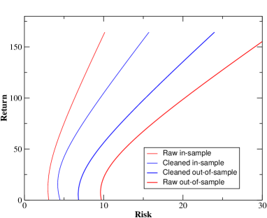
Figure 1: In sample (left curves) and out of sample (right curves) portfolio risk along the optimal curve in the risk return plane. Red lines are with the raw empirical matrix, blue lines with the cleaned matrix using RMT, showing how the risk underestimation can be reduced by matrix cleaning. From dublin .

II Matrix cleaning and RMT

How should one ‘clean’ the empirical correlation matrix to avoid, as much as possible, such biases in the estimation of future risk? In order to get some general intuition on this problem, let us rewrite the Markowitz solution in terms of the eigenvalues $\lambda_{k}$ and eigenvectors $V_{i}^{k}$ of the correlation matrix:

$$w_{i}\propto\sum_{kj}\lambda_{k}^{-1}V_{i}^{k}V_{j}^{k}g_{j}\equiv g_{i}+\sum_{kj}(\lambda_{k}^{-1}-1)V_{i}^{k}V_{j}^{k}g_{j}$$ (14)

The first term corresponds to the naive solution: one should invest proportionally to the expected gain (in units where $\sigma_{i}=1$). The correction term means that the weights of eigenvectors with $\lambda>1$ are suppressed, whereas the weights of eigenvectors with $\lambda<1$ are enhanced. Potentially, the optimal Markowitz solution allocates a very large weight to small eigenvalues, which may be entirely dominated by measurement noise and hence unstable. A very naive way to avoid this is to go for the naive solution $w_{i}\propto g_{i}$, but with the $k^{*}$ largest eigenvectors projected out:

$$w_{i}\propto g_{i}-\sum_{k\leq k^{*};j}V_{i}^{k}V_{j}^{k}g_{j},$$ (15)

so that the portfolio is market neutral (the largest eigenvector correspond to a collective market mode, $V_{i}^{1}\approx 1/\sqrt{N}$) and sector neutral (other large eigenvectors contain sector moves). Since most of the volatility is contained in the market and sector modes, the above portfolio is already quite good in terms of risk. More elaborated ways aim at retaining all eigenvalues and eigenvectors, but after having somehow cleaned them. A well known cleaning corresponds to the so-called “shrinkage estimator”: the empirical matrix is shifted ‘closer’ to the identity matrix. This is a Bayesian method that assumes that the prior empirical matrix is the identity, again only justified if the market mode has been subtracted out. More explicitely:

$$\mathbf{E}_{c}=\alpha\mathbf{E}+(1-\alpha)\mathbf{1}\qquad\mbox{{so}}\qquad\lambda^{k}_{c}=1+\alpha(\lambda^{k}-1),$$ (16)

where the subscript $c$ corresponds to the cleaned objects. This method involves the parameter $\alpha$ which is undetermined, but somehow related to the expected signal to noise ratio. If the signal is large, $\alpha\to 1$, and $\alpha\to 0$ if the noise is large. Another possible interpretation is through a constraint on the effective number of assets in the portfolio, defined as $(\sum_{i}w_{i}^{2})^{-1}$ book . Constraining this number to be large (ie imposing a minimal level of diversification) is equivalent to choosing $\alpha$ small.

Another route is eigenvalue cleaning, first suggested in prl ; dublin , where one replaces all low lying eigenvalues with a unique value, and keeps all the high eigenvalues corresponding to meaningful economical information (sectors):

$$\lambda^{k}_{c}=1-\delta\qquad\mbox{{if}}\qquad k>k^{*},\qquad\lambda^{k}_{c}=\lambda^{k}_{E}\qquad\mbox{{if}}\qquad k\leq k^{*},$$ (17)

where $k^{*}$ is the number of meaningful number of sectors and $\delta$ is chosen such that the trace of the correlation matrix is exactly preserved. How should $k^{*}$ be chosen? The idea developed in prl ; dublin is to use Random Matrix Theory to determine the theoretical edge of the ‘random’ part of the eigenvalue distribution, and to fix $k^{*}$ such that $\lambda^{k^{*}}_{E}$ is close to this edge.

What is then the spectrum of a random correlation matrix? The answer is known in several cases, due to the work of Marčenko and Pastur marcenkopastur and others baisilverstein ; sengupta ; burdagorlich . We briefly recall the results and some elegant methods to derive them, with special emphasis on the problem of the largest eigenvalue, which we expand on below. Consider an empirical correlation matrix $\mathbf{E}$ of $N$ assets using $T$ data points, both very large, with $q=N/T$ finite. Suppose that the true correlations are given by $\langle x^{i}_{t}x^{j}_{t^{\prime}}\rangle=C_{ij}\delta_{tt^{\prime}}$. This defines the Wishart ensemble Wishart . In order to find the eigenvalue density, one introduces the resolvent:

$$G(z)=\frac{1}{N}\mbox{Tr}\left[(z\mathbf{I}-\mathbf{E})^{-1}\right]$$ (18)

from which one gets:

$$\rho(\lambda)=\lim_{\epsilon\to 0}\frac{1}{\pi}\Im\left(G(\lambda-\mbox{i}\epsilon)\right).$$ (19)

The simplest case is when $\mathbf{C}=\mathbf{I}$. Then, $\mathbf{E}$ is a sum of rotationally invariant matrices $\delta E^{t}_{ij}=(x^{i}_{t}x^{j}_{t})/T$. The trick in that case is to consider the so-called Blue function, inverse of $G$, i.e. such that $B(G(z))=z$. The quantity $R(x)=B(x)-1/x$ is the ‘R-transform’ of $G$, and is known to be additive marcenkopastur ; voiculescu ; zee . Since $\delta\mathbf{E}^{t}$ has one eigenvalue equal to $q$ and $N-1$ zero eigenvalues, one has:

$$\delta G_{t}(z)=\frac{1}{N}\left(\frac{1}{z-q}+\frac{N-1}{z}\right)$$ (20)

Inverting $\delta G_{t}(z)$ to first order in $1/N$,

$$\delta B_{t}(x)=\frac{1}{x}+\frac{q}{N(1-qx)}\quad\longrightarrow\quad B_{E}(x)=\frac{1}{x}+\frac{1}{(1-qx)},$$ (21)

and finally

$$G_{E}(z)=\frac{(z+q-1)-\sqrt{(z+q-1)^{2}-4zq}}{2zq},$$ (22)

which finally reproduces the well known Marčenko-Pastur (MP) result:

$$\rho(\lambda)=\frac{\sqrt{4\lambda q-(\lambda+q-1)^{2}}}{2\pi\lambda q}$$ (23)

The case of a general $\mathbf{C}$ cannot be directly written as a sum of “Blue” functions, but one can get a solution using the Replica trick or by summing planar diagrams, which gives the following relation between resolvents: baisilverstein ; sengupta ; burdagorlich

$$zG_{E}(z)=ZG_{C}(Z)\qquad\mbox{{where}}\qquad Z=\frac{z}{1+q(zG_{E}(z)-1)},$$ (24)

from which one can easily obtain $\rho(\lambda)$ numerically for any choice of $\mathbf{C}$ burdagorlich . [In fact, this result can even be obtained from the original Marčenko-Pastur paper by permuting the role of the appropriate matrices]. The above result does however not apply when $\mathbf{C}$ has isolated eigenvalues, and only describes continuous parts of the spectrum. For example, if one considers a matrix $\mathbf{C}$ with one large eigenvalue that is separated from the ‘Marčenko-Pastur sea’, the statistics of this isolated eigenvalue has recently been shown to be Gaussian BenArous (see also below), with a width $\sim T^{-1/2}$, much smaller than the uncertainty on the bulk eigenvalues ($\sim q^{1/2}$). A naive application of Eq. (24), on the other hand, would give birth to a ‘mini-MP’ distribution around the top eigenvalue. This would be the exact result only if the top eigenvalue of $C$ had a degeneracy proportional to $N$.

From the point of view of matrix cleaning, however, these results show that: (i) the expected edge of the bulk, that determines $k^{*}$, obviously depends on the prior one has for $\mathbf{C}$. The simplest case where $\mathbf{C}=\mathbf{I}$ was investigated in particular in prl ; Plerou , with the results shown in Fig 2. Other choices are however possible and could lead to an improved cleaning algorithm; (ii) the uncertainty on large eigenvalues is much less than that on the bulk eigenvalues, meaning that the bulk needs a lot of shrinkage, but the bigger eigenvalues less so – at variance with the naive shrinkage procedure explained above. An alternative route may consist in using the ‘power mapping’ method proposed by Guhr Guhr or clustering methods Lillo .

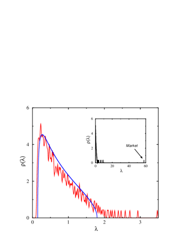
Figure 2: Empirical eigenvalue density for 406 stocks from the S&P 500, and fit using the MP distribution. Note (i) the presence of one very large eigenvalue, corresponding to the market mode (see section IV) and (ii) the MP fit reveals systematic deviations, suggesting a non trivial structure of the true correlation matrix, even after sector modes have been accounted for (see burdagorlich ; us ).

III EWMA Empirical Correlation Matrices

Consider now the case where $\mathbf{C}=\mathbf{I}$ but where the Empirical matrix is computed using an exponentially weighted moving average (EWMA). More precisely:

$$E_{ij}=\epsilon\sum_{t^{\prime}=-\infty}^{t-1}(1-\epsilon)^{t-t^{\prime}}x_{i}^{t^{\prime}}x_{j}^{t^{\prime}}$$ (25)

with $\epsilon=1/T$. Such an estimate is standard practice in finance. Now, as an ensemble $E_{ij}$ satisfies $E_{ij}=(1-\epsilon)E_{ij}+\epsilon x_{i}^{t}x_{j}^{t}$. We again invert the resolvent of $\delta\mathbf{E_{t}}$ to find the elementary R-function,

$$\delta B_{t}(x)=\frac{1}{x}+R_{t}(x)\qquad\mbox{{with}}\qquad R_{t}(x)=\frac{q}{N(1-qx)}$$ (26)

Using the scaling properties of $G(z)$ we find for $R(x)$:

$$R_{aC}(x)=aR_{C}(ax).$$ (27)

This allows one to write:

$$R_{E}(x)=R_{(1-\epsilon)E}(x)+R_{t}(x)=(1-q/N)R_{E}((1-q/N)x)+\frac{q}{N(1-qx)}$$ (28)

To first order in $1/N$, one now gets:

$$R(x)+xR^{\prime}(x)+\frac{q}{1-qx}=0\longrightarrow R(x)=-\frac{\log(1-qx)}{qx}.$$ (29)

Going back to the resolvent to find the density, we finally get the result first obtained in PKP :

$$\rho(\lambda)=\frac{1}{\pi}\Im G(\lambda)\quad\mbox{{ where $G(\lambda)$ solves }}\quad\lambda qG=q-\log(1-qG)$$ (30)

This solution is compared to the standard MP distribution in Fig 3.

Another nice properties of Blue functions is that they can be used to find the edges of the eigenvalue spectrum ($\lambda_{\pm}$). One has:zee

$$\lambda_{\pm}=B(x_{\pm})\qquad\mbox{where}\qquad B^{\prime}(x_{\pm})=0$$ (31)

In the case at hand, by evaluating $B(x)$ when $B^{\prime}(x)=0$ we can write directly an equation whose solutions are the spectrum edges ($\lambda_{\pm}$)

$$\lambda_{\pm}=\log(\lambda_{\pm})+q+1$$ (32)

When $q$ is zero, the spectrum is a $\delta$ in $1$ as expected. But as the noise increases (or the characteristic time decreases) the lower edge approach zero very quickly as $\lambda_{-}\sim\exp(-q)$. Although there are no exact zero eigenvalues for EWMA matrices, the smallest eigenvalue is very close to zero.

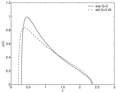
Figure 3: Spectrum of the exponentially weighted random matrix with $q\equiv N\epsilon=1/2$ and the spectrum of the standard Wishart random matrix with $q\equiv N/T=1/3.45$, chosen to have the same upper edge. From PKP .

IV Dynamics of the top eigenvalue and eigenvector

As mentioned above, it is well known that financial covariance matrices are such that the largest eigenvalue is well separated from the ‘bulk’, where all other eigenvalues reside. The financial interpretation of this large eigenvalue is the so-called ‘market mode’: in a first approximation, all stocks move together, up or down. One can state this more precisely in the context of the one factor model, where the $i$th stock return at time $t$ is written as:

$$r_{t}^{i}=\beta_{i}\phi_{t}+\varepsilon_{t}^{i},$$ (33)

where the market mode $\phi_{t}$ is common to all stocks through their market exposure $\beta^{i}$ and the $\varepsilon_{t}^{i}$ are idiosyncratic noises, uncorrelated from stock to stock. Within such a model, the covariance matrix reads:

$$C_{ij}=\beta_{i}\beta_{j}\sigma_{\phi}^{2}+\sigma_{i}^{2}\delta_{ij}.$$ (34)

When all $\sigma_{i}$’s are equal, this matrix is easily diagonalized; for $N$ stocks, its largest eigenvalue is $\Lambda_{0}=(\sum_{j}\beta_{j}^{2})\sigma_{\phi}^{2}+\sigma^{2}$ and is of order $N$, and all the other $N-1$ eigenvalues $\Lambda_{\alpha}$ are equal to $\sigma^{2}$. The largest eigenvalue corresponds to the eigenvector $\beta_{i}$. More generally, the largest eigenvalue $\Lambda_{0}$, normalized by the average square volatility of the stocks, can be seen as a proxy for the average interstock correlation.

A natural question, of great importance for portfolio management, or dispersion trading (option strategies based on the implied average correlation between stocks), is whether $\Lambda_{0}$ and the $\beta$’s are stable in time. Of course, the largest eigenvalue and eigenvector of the empirical correlation matrix will be, as discussed at length above, affected by measurement noise. Can one make predictions about the fluctuations of both the largest eigenvalue and the corresponding eigenvector induced by measurement noise? This would help separating a true evolution in time of the average stock correlation and of the market exposure of each stock from one simply related to measurement noise. We shall see that such a decomposition seems indeed possible in the limit where $\Lambda_{0}\gg\Lambda_{\alpha}$.

We will assume, as in the previous section, that the covariance matrix is measured through an exponential moving average of the returns. This means that the matrix ${\mathbf{E}}$ evolves in time as:

$$E_{ij,t}=(1-\epsilon)E_{ij,t-1}+\epsilon r_{t}^{i}r_{t}^{j}.$$ (35)

The true covariance matrix $C_{ij}=\langle r^{i}r^{j}\rangle$ is assumed to be time independent – this will give us our benchmark hypothesis – with its largest eigenvalue $\Lambda_{0}$ associated to the normalized eigenvector $\Psi_{0}$. In this section we deal with covariance matrices instead of correlation matrices for simplicity, but most results should carry over to this latter case as well.

Denoting as $\lambda_{0t}$ the largest eigenvalue of $E_{t}$ associated to $\psi_{0t}$, standard perturbation theory, valid for $\epsilon\ll 1$, gives:

$$\lambda_{0t}=(1-\epsilon)\lambda_{0t-1}+\epsilon\langle\psi_{0t-1}|C|\psi_{0t-1}\rangle+\epsilon\langle\psi_{0t-1}|\eta_{t}|\psi_{0t-1}\rangle,$$ (36)

with $\eta_{ij}=r^{i}r^{j}-\langle r^{i}r^{j}\rangle$. We will suppose for simplicity that the returns are Gaussian, yielding:

$$\langle\eta_{ij}\eta_{k\ell}\rangle=C_{ik}C_{j\ell}+C_{i\ell}C_{jk}.$$ (37)

In the limit where $\Lambda_{0}$ becomes much larger than all other eigenvectors, the above equation simplifies to:

$$\lambda_{0t}\approx(1-\epsilon)\lambda_{0t-1}+\epsilon\cos^{2}\theta_{t-1}\Lambda_{0}\left[1+\xi_{t}\right],$$ (38)

where $\cos\theta_{t}\equiv\langle\psi_{0t}|\Psi_{0}\rangle$ and $\xi_{t}$ is a random noise term of mean zero and variance equal to $2$. This noise becomes Gaussian in the limit of large matrices, leading to a Langevin equation for $\lambda_{0}$:

$$\frac{d\lambda_{0}}{dt}=\epsilon(\cos^{2}\theta\Lambda_{0}-\lambda_{0})+\epsilon\cos^{2}\theta\xi_{t}.$$ (39)

We have neglected in the above equation a deterministic term equal to $\epsilon\sin^{2}\theta\Lambda_{1}$, which will turn out to be a factor $(\Lambda_{1}/\Lambda_{0})^{2}$ smaller than the terms retained in Eq. (38).

We now need to work out an equation for the projection of the instantaneous eigenvector $\psi_{0t}$ on the true eigenvector $\Psi_{0}$. This can again be done using perturbation theory, which gives, in braket notation:

$$|\psi_{0t}\rangle = |\psi_{0t-1}\rangle+\epsilon\sum_{\alpha\neq 0}\frac{\langle\psi_{\alpha t-1}|r_{t}r_{t}|\psi_{0t-1}\rangle}{\lambda_{0t-1}-\lambda_{\alpha t-1}}|\psi_{\alpha t-1}\rangle$$ (40)

$$\approx |\psi_{0t-1}\rangle+\epsilon\frac{r_{t}r_{t}|\psi_{0t-1}\rangle}{\lambda_{0t-1}}-\epsilon\frac{\langle\psi_{0t-1}|r_{t}r_{t}|\psi_{0t-1}\rangle}{\lambda_{0t-1}}|\psi_{0t-1}\rangle,$$

where we have used the fact that the basis of eigenvectors is complete. It is clear by inspection that the correction term is orthogonal to $|\psi_{0t-1}\rangle$, so that $|\psi_{0t}\rangle$ is still, to first order in $\epsilon$, normalized. Let us now decompose the matrix $r_{t}r_{t}$ into its average part $C$ and the fluctuations $\eta$, and first focus on the former contribution. Projecting the above equation on $<\Psi_{0}|$ leads to the deterministic part of the evolution equation for $\cos\theta_{t}$:

$$\cos\theta_{t}\approx\cos\theta_{t-1}+\epsilon\cos\theta_{t-1}\frac{\Lambda_{0}}{\lambda_{0t-1}}-\epsilon\cos^{3}\theta_{t-1}\frac{\Lambda_{0}}{\lambda_{0t-1}},$$ (41)

where we have neglected the contribution of the small eigenvalues compared to $\Lambda_{0}$, which is again a factor $(\Lambda_{1}/\Lambda_{0})^{2}$ smaller. In the continuous time limit $\epsilon\to 0$, this equation can be rewritten as:

$$\frac{d\theta}{dt}=-\frac{\epsilon\Lambda_{0}}{2\lambda_{0t}}\sin 2\theta,$$ (42)

and describes a convergence of the angle $\theta$ towards $0$ or $\pi$ – clearly, $\Psi_{0}$ and $-\Psi_{0}$ are equivalent. It is the noise term $\eta$ that will randomly push the instantaneous eigenvector away from its ideal position, and gives to $\theta$ a non-trivial probability distribution. Our task is therefore to compute the statistics of the noise, which again becomes Gaussian for large matrices, so that we only need to compute its variance. Writing $|\psi_{0t}\rangle=\cos\theta_{t}|\Psi_{0}\rangle+\sin\theta_{t}|\Psi_{1t}\rangle$, where $|\Psi_{1t}\rangle$ is in the degenerate eigenspace corresponding to small eigenvalues $\Lambda_{1}$, and using Eq. (37), we find that the noise term $\zeta_{t}$ to be added to Eq. (42) is given by:

$$\langle\zeta_{t}^{2}\rangle\approx\frac{\epsilon^{2}}{\lambda_{0t}^{2}}\left[2\Lambda_{0}^{2}\cos^{2}\theta_{t}\sin^{2}\theta_{t}+\Lambda_{0}\Lambda_{1}\cos^{2}2\theta_{t}\right],$$ (43)

where we have kept the second term because it becomes the dominant source of noise when $\theta\to 0$, but neglected a term in $\Lambda_{1}^{2}$. The eigenvector $\psi_{0}$ therefore undergoes an Ornstein-Uhlenbeck like motion on the unit sphere. One should also note that the two sources of noise $\xi_{t}$ and $\zeta_{t}$ are not independent. Rather, one has, neglecting $\Lambda_{1}^{2}$ terms:

$$2\langle\xi_{t}\zeta_{t}\rangle\approx\Lambda_{0}\cos^{2}\theta_{t}\sin 2\theta_{t}-\Lambda_{1}\sin 4\theta_{t}$$ (44)

In the continuous time limit, we therefore have two coupled Langevin equations for the top eigenvalue $\lambda_{0t}$ and the deflection angle $\theta_{t}$. In the limit $\Lambda_{1}\ll\Lambda_{0}$, the stationary solution for the angle can be computed to be:

$$P(\theta)={\cal N}\left[\frac{1+\cos 2\theta(1-\frac{\Lambda_{1}}{\Lambda_{0}})}{1-\cos 2\theta(1-\frac{\Lambda_{1}}{\Lambda_{0}})}\right]^{1/4\epsilon}$$ (45)

As expected, this distribution is invariant when $\theta\to\pi-\theta$, since $-\Psi_{0}$ is also a top eigenvector. In the limit $\Lambda_{1}\ll\Lambda_{0}$, one sees that the distribution becomes peaked around $\theta=0$ and $\pi$. For small $\theta$, the distribution becomes Gaussian:

$$P(\theta)\approx\frac{1}{\sqrt{2\pi\epsilon\frac{\Lambda_{1}}{\Lambda_{0}}}}\exp\left(-\frac{\theta^{2}}{2\epsilon\frac{\Lambda_{1}}{\Lambda_{0}}}\right),$$ (46)

leading to $\langle\cos^{2}\theta\rangle\approx 1-\epsilon{\Lambda_{1}}/2{\Lambda_{0}}$ The angle $\theta$ is less and less fluctuating as $\epsilon\to 0$ (as expected) but also as $\Lambda_{1}/\Lambda_{0}\to 0$: a large separation of eigenvalues leads to a well determined top eigenvector. In this limit, the distribution of $\lambda_{0}$ also becomes Gaussian (as expected from general results BenArous ) and one finds, to leading order:

$$\langle\lambda_{0}\rangle\approx\Lambda_{0}-\epsilon{\Lambda_{1}}/2;\qquad\langle(\delta\lambda_{0})^{2}\rangle\approx\epsilon.$$ (47)

Therefore, we have shown that in the limit of large averaging time and one large top eigenvalue (a situation approximately realized for financial markets), the deviation from the true top eigenvalue $\delta\lambda_{0}$ and the deviation angle $\theta$ are independent Gaussian variables (the correlation between them indeed becomes zero as can be seen using Eq. (44) in that limit, both following Ornstein-Uhlenbeck processes.

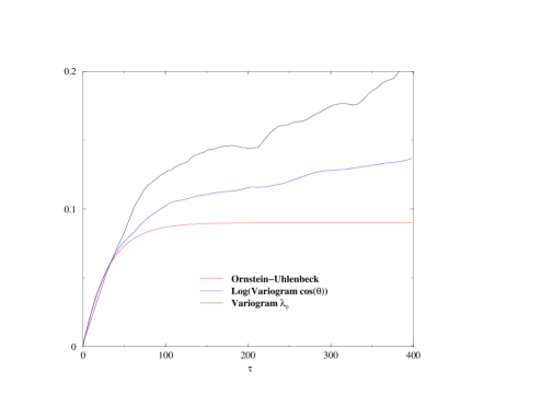
Figure 4: Variogram of the top eigenvalue of the correlation matrix $\lambda_{0}$ (top curve) and (log)-variogram of the top eigenvector, $\ln\left\langle\langle\psi_{0t+\tau}|\psi_{0t}\rangle\right\rangle$, as a function of the time lag $\tau$, for US stocks, and for an exponential moving average parameter $\epsilon=1/30$ days. We show for comparison (bottom curve) the Ornstein-Uhlenbeck behaviour expected for both quantities in the case of a time independent underlying correlation structure.

From these results one directly obtains the variogram of the top eigenvalue as:

$$\langle[\lambda_{t+\tau}-\lambda_{t}]^{2}\rangle=2\epsilon\left(1-\exp(-\epsilon\tau)\right).$$ (48)

This is the result expected in the absence of a ‘true’ dynamical evolution of the structure of the matrix. From Fig. 4, one sees that there is clearly an additional contribution, hinting at a real evolution of the strength of the average correlation with time. One can also work out the average overlap of the top eigenvector with itself as a function of time lag, $E(\langle\psi_{0t+\tau}|\psi_{0t}\rangle)$. Writing again $|\psi_{0t}\rangle=\cos\theta_{t}|\Psi_{0}\rangle+\sin\theta_{t}|\Psi_{1t}\rangle$, one sees that an equation for the evolution of the transverse component $|\Psi_{1t}\rangle$ is a priori also needed. It is easy to show, following the same method as above, that the evolution of the angle $\phi_{t}$ made by the component with a fixed direction is a free diffusion with a noise term of order $\epsilon\Lambda_{1}/\Lambda_{0}$. Therefore, on the time scale $\epsilon^{-1}$ over which $\theta_{t}$ evolves, $|\Psi_{1t}\rangle$ can be considered to be quasi-constant, leading to:

$$\left\langle\langle\psi_{0t+\tau}|\psi_{0t}\rangle\right\rangle\approx E(\cos(\theta_{t}-\theta_{t+\tau}))\approx 1-\epsilon\frac{\Lambda_{1}}{\Lambda_{0}}(1-\exp(-\epsilon\tau)).$$ (49)

Any significant deviation from the above law would, again, indicate a true evolution of the market structure. Again, Fig. 4, provides some evidence of such an evolution, although weaker than that of the top eigenvalue $\lambda_{0}$.

V Frequency dependent correlation matrices

The very definition of the correlation matrix a priori depends on the time scale over which returns are measured. The return on time $\tau$ for stock $i$ is defined as: $r_{i,\tau}(t)=\ln p_{i}(t+\tau)-\ln p_{i}(t)$, where $p_{i}(t)$ is the price at time $t$. The correlation matrix is then defined as:

$$C_{ij}(\tau)=\frac{\langle r_{i,\tau}(t)r_{j,\tau}(t)\rangle_{c}}{\sigma_{i}\sigma_{j}}$$ (50)

A relatively well known effect is that the average inter-stock correlation grows with the observation time scale – this is the so-called Epps effect Epps ; Reno . For example, for a collection of stocks from the FTSE index, one finds, in the period 1994-2003:

$$\langle C_{i\neq j}(5^{\prime})\rangle\approx 0.06;\qquad\langle C_{i\neq j}(1h)\rangle\approx 0.19;\qquad\langle C_{i\neq j}(1d)\rangle\approx 0.29$$ (51)

Besides the change of the average correlation level, there is also a change of structure of the correlation matrix: the full eigenvalue distribution distribution changes with $\tau$. A trivial effect is that by increasing the observation frequency one also increases the number of observations; the parameter $q$ defined above decreases and the noise band is expected to shrink. This, at first sight, appears to be a nice way to get rid of the observation noise in the correlation matrix (see Iori for a related discussion). Unfortunately, the problem (or the interesting effect, depending on the standpoint) is that this is accompanied by a true modification of the correlations, for which we will provide a model below. In particular one observes the emergence of a larger number of eigenvalues leaking out from the bulk of the eigenvalue spectrum (and corresponding to ‘sectors’) as the time scale $\tau$ increases. This effect was also noted by Mantegna Mantegna : the structure of the minimal spanning tree constructed from the correlation matrix evolves from a ‘star like’ structure for small $\tau$’s (several minutes), meaning that only the market mode is present, to a fully diversified tree at the scale of a day. Pictorially, the market appears as an embryo which progressively forms and differentiates with time.

The aim of this section is to introduce a simple model of lagged cross-influences that allows one to rationalize the mechanism leading to such an evolution of the correlation matrix. Suppose that the return of stock $i$ at time $t$ is influenced in a causal way by return of stock $j$ at all previous times $t^{\prime}<t$. The most general linear model for this reads:

$$r_{i,1}(t)=\xi_{i}(t)+\sum_{j}\int_{-\infty}^{t}{\rm d}t^{\prime}K_{ij}(t-t^{\prime})r_{j,1}(t^{\prime})\qquad\langle\xi_{i}(t)\xi_{j}(t^{\prime})\rangle=D_{i}\delta_{ij}\delta(t-t^{\prime})$$ (52)

Here $\tau=1$ is the shortest time scale – say a few seconds. The kernel $K_{ij}$ is in general non-symmetric and describes how the return of stock $j$ affects, on average, that of stock $i$ a certain time later. We will define the lagged correlation ${\cal C}_{ij}(t-t^{\prime})$ by:

$${\cal C}_{ij}(t-t^{\prime})=\langle r_{i,1}(t)r_{j,1}(t^{\prime})\rangle.$$ (53)

This matrix is, for $t\neq t^{\prime}$, not symmetric; however, one has obviously ${\cal C}_{ij}(t-t^{\prime})={\cal C}_{ji}(t^{\prime}-t)$. These lagged correlations were already studied in Kertesz . Going to Fourier space, one finds the Fourier transform of the covariance matrix ${\cal C}_{ij}(\omega)={\cal C}_{ji}(-\omega)$:

$${\cal C}_{ij}(\omega)=\sum_{k}(1-K(\omega))^{-1}_{ik}(1-K(-\omega))^{-1}_{jk}D_{k}$$ (54)

where $K(\omega)$ is the Fourier transform of $K(\tau)$ with by convention $K(\tau<0)=0$. When cross-correlations are small, which is justified provided the $r_{i,1}(t)$ corresponds to residual returns, where the market has been subtracted, the relation between ${\cal C}_{ij}$ and $K_{ij}$ becomes quite simple and reads, for $\tau>0$:

$${\cal C}_{ij}(\tau)=D_{j}K_{ij}(\tau).$$ (55)

This equation allows one, in principle, to determine $K_{ij}(\tau)$ from the empirical observation of the lagged correlation matrix. Suppose for simplicity that the influence kernel takes the form $K_{ij}(\tau)=K_{ij}^{0}e^{-\Gamma_{ij}\tau}$, then $K_{ij}(\omega)=K_{ij}^{0}/(i\omega+\Gamma_{ij})$. In this model, the primary object is the influence matrix $K$ which has a much richer structure than the correlation matrix: each element defines an influence strength $K^{0}$ and an synchronisation time $\Gamma^{-1}$. In fact, as shown in Figs. 5 and 6, fitting the empirical data requires that $K_{ij}$ is parameterized by a sum of at least two exponentials, one corresponding to a time scale of minutes, and a second one of hours; sometimes the influence strength corresponding to these two time scales have opposite signs. Pooling together the parameters corresponding to different pairs of stocks, we find, as might have been expected, that strongly coupled stocks (large $K^{0}$) have short synchronisation times $\Gamma^{-1}$.

Figure 5: Typical self-influence kernel $K_{ii}(E)$ in Laplace space and fit with the Laplace transforms of the sum of two exponentials.

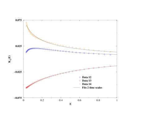
Figure 6: Typical cross-influence kernels $K_{ij}(E)$ for three pairs of stocks, and fit with the Laplace transforms of the sum of two exponentials. Note that the influence amplitudes have different signs, even for the same pair of stock, depending on the time scale.

Coming back to the observation that the correlation matrix is frequency dependent, one should note that the scale dependent correlation matrix $C_{ij}(\tau)$ is related to ${\cal C}_{ij}(\omega)$ by:

$$C_{ij}(\tau)=\langle r_{i,\tau}r_{j,\tau}\rangle_{c}=\int\ d\omega\ S^{2}(\omega\tau){\cal C}_{ij}(\omega)$$ (56)

where $S(.)$ is the form factor (i.e. Fourier transform of the window used to define returns on scale $\tau$, for example a flat window in the simplest case). Therefore, for $\tau$ small one finds that residuals are uncorrelated (i.e. the correlation matrix has no structure beyond the market mode):

$$C_{ij}(\tau\to 0)\approx D_{i}\delta_{ij},$$ (57)

whereas on long time scales the full correlation develops as:

$$C_{ij}(\tau\to\infty)\approx D_{i}\delta_{ij}+\int_{0}^{\infty}{\rm d}\tau\left[D_{j}K_{ij}(\tau)+D_{i}K_{ji}(\tau)\right].$$ (58)

The emergence of correlation structure therefore reveals the lagged cross-influences in the market. Note that on long time scales, small $K^{0}$’s can be counterbalanced by large synchronisation times $\Gamma^{-1}$, and lead to significant correlations between ‘weakly coupled’ stocks.

We believe that a more systematic empirical study of the influence matrix $K_{ij}$ and the way it should be cleaned, in the spirit of the discussion in section II, is worth investigating in details.

We want to thank Pedro Fonseca and Boris Schlittgen for many discussions on the issues addressed in sections IV and V, and Szilard Pafka and Imre Kondor for sharing the results on the EWMA matrices given in section III. We also thank Gérard Ben Arous and Jack Silverstein for several clarifying discussions. We also thank the organisers of the meeting in Cracow for inviting us and for making the conference a success.

References

- (1) L. Laloux, P. Cizeau, J.-P. Bouchaud and M. Potters, Phys. Rev. Lett. 83, 1467 (1999); L. Laloux, P. Cizeau, J.-P. Bouchaud and M. Potters, Risk 12, No. 3, 69 (1999).
- (2) J.-P. Bouchaud and M. Potters, Theory of Financial Risk and Derivative Pricing (Cambridge University Press, 2003).
- (3) S. Pafka, I. Kondor, Physica A319 487 (2003) and cond-mat/0305475
- (4) L. Laloux, P. Cizeau, J.-P. Bouchaud and M. Potters, Int. J. Theor. Appl. Finance 3, 391 (2000).
- (5) V. A. Marčenko and L. A. Pastur, Math. USSR-Sb, 1, 457-483 (1967).
- (6) J. W. Silverstein and Z. D. Bai, Journal of Multivariate Analysis, 54 175 (1995).
- (7) A. N. Sengupta and P. Mitra, Phys. Rev. E 80, 3389 (1999).
- (8) Z. Burda, A. Görlich, A. Jarosz and J. Jurkiewicz, Physica A, 343, 295-310 (2004).
- (9) J. Wishart, Biometrika, A20 32 (1928).
- (10) V. Plerou, P. Gopikrishnan, B. Rosenow, L. N. Amaral, H. E. Stanley, Phys. Rev. Lett. 83, 1471 (1999).
- (11) D. V. Voiculescu, K. J. Dykema, A. Nica, Free Random Variables, AMS, Providence, RI (1992).
- (12) A. Zee, Nuclear Physics B 474, 726 (1996)
- (13) J. Baik, G. Ben Arous, and S. Peche, Phase transition of the largest eigenvalue for non-null complex sample covariance matrices, http://xxx.lanl.gov/abs/math.PR/0403022, to appear in Ann. Prob, and these proceedings
- (14) T. Guhr, B. Kalber, J. Phys. A 36, 3009 (2003), and these proceedings.
- (15) F. Lillo, R. Mantegna, Cluster analysis for portfolio optimisation, these proceedings, and physics/0507006.
- (16) M. Potters, J. P. Bouchaud, Embedded sector ansatz for the true correlation matrix in stock markets, in preparation.
- (17) S. Pafka, I. Kondor, M. Potters, Exponential weighting and Random Matrix Theory based filtering of financial covariance matrices, cond-mat/0402573, to appear in Quantitative Finance.
- (18) T. Epps, Comovement of stock prices in the very short run, J. Am. Stat. Assoc. 74, 291 (1979)
- (19) R. Reno, Int. Journ. Th. Appl. Fin, 6, 87 (2003)
- (20) O. Precup, G. Iori, A comparison of high frequency cross correlation measures, preprint.
- (21) G. Bonanno, N. Vandewalle and R. N. Mantegna, Physical Review E62 R7615-R7618 (2001)
- (22) L. Kullman, J. Kertesz, T. Kaski, Phys. Rev. E66 026125 (2002)