Production networks and failure avalanches

Abstract

Although standard economics textbooks are seldom interested in production networks, modern economies are more and more based upon suppliers/customers interactions. One can consider entire sectors of the economy as generalised supply chains. We will take this view in the present paper and study under which conditions local failures to produce or simply to deliver can result in avalanches of shortage and bankruptcies across the network. We will show that a large class of models exhibit scale free distributions of production and wealth among firms and that metastable regions of high production are highly localised.

1 Networks of firms

Firms are not simply independent agents competing for customers on markets. Their activity involves many interactions, and some of them even involve some kind of cooperation. Interactions among firms might include:

• information exchange[3][4],[5];

• loans[7],[8];

• common endeavours[9];

• partial ownership[6];

• and of course economic transactions allowing production[10] (the present paper).

Economic activity can be seen as occurring on an economic network (“le tissu économique”): firms are represented by vertices and their interactions by edges. The edges are most often asymmetric (think for instance of providers/customers interactions). The availability of empirical data has provoked research on the structure of these networks: many papers discuss their “small world properties”[1] and frequently report scale free distribution[2] of the connections among firms.

The long term interest of economic network research is rather the dynamics creating or occurring on these nets: how are connections evolving, what are the fluxes of information, decisions[4],[5], economic transactions etc … But dynamic studies lag behind statistical approaches because of conceptual difficulties and because time series of individual transactions are harder to obtain than time aggregated statistics.

The recent cascade of bankruptcies that occurred in Eastern Asia in 1997, provoked some research on the influence of the loans network structure on the propagation of “bad debts” and resulting avalanches of bankruptcies ([7],[8]) . One of the most early papers on avalanche distribution in economic networks is due to Bak et al [10]. It concerns production networks: edges represent suppliers/customers connections among firms engaged in batch production activity. The authors describe the distribution of production avalanches triggered by random independent demand events at the output boundary of the production network.

These papers ([7],[8] and[10]) are not based on any empirical description of the network structure, but assume a very simple interaction structure: star structure in the first case[7],[8], periodic lattice in Bak et al paper[10]. They neither take into account price dynamics.

The present paper is along these lines: we start from a very simple lattice structure and we study the consequences of simple local processes of orders/production (with or without failure)/delivery/ profit/investment on the global dynamics: evolution of global production and wealth in connection to their distribution and local patterns. In the spirit of complex systems analysis, our aim is not to present specific economic prediction, but primarily to concentrate on the generic properties (dynamical regimes, transitions, scaling laws) common to a large class of models of production networks.

A minimal model of a production network will first be introduced in section 2. Simulation results are presented in section 3. Section 4 is a discussion of the genericity of the obtained results: reference is made to comparable soluble models. We also summarise the results of several variants of the simplest model. The conclusion is a discussion of possible applications to geographical economics.

2 A simple model of a production network

We can schematise the suppliers/customers interactions among firms by a production network, where firms are located at the vertices and directed edges represent the delivery of products from one firm to its customers (see figure 1).

Independent local failures to produce (or to deliver) by a firm might give rise to the propagation of shortage across the production network.

Figure 1: Firms are located at the nodes of the lattice. Production ($Y^{D}$) flows from the resource input layer ($k=l)$ to the output layer ($k=0$), orders ($Y$) flow backward.

We have chosen a simple periodic lattice with three input connections of equal importance and three output per firm. The network is oriented from an input layer (say natural resources) towards an output layer (say the shelves of supermarkets). The transverse axis can be thought as representing either geographical position or some product space while the longitudinal axis relates to production. We here use a one dimensional transverse space to facilitate the representation of the dynamics by two-dimensional patterns, but there is no reason to suppose geographical or product space to be one-dimensional in the real world.

In real economies, the network structure is more heterogenous with firms of unequal importance and connectivity. Furthermore some delivery connections go backwards. Most often these backward connections concern equipment goods; neglecting them as we do here implies considering equipment goods dynamics as much slower than consumption goods dynamics. Anyway, since these backward connections enter positive feedback loops, we have no reason to suppose that they would qualitatively disrupt the dynamics that we further describe.

At each time step two opposite flows get across the lattice: orders are first transmitted upstream from the output layer; production is then transmitted downstream from the input layer to the output layer.

• Orders at the output layer

  We suppose that orders are only limited by the production capacity $A_{0i}$ of the firm in position ${0,i}$, where $0$ indicates the output layer, and $i$ the transverse position in the layer.

  $$Y_{0i} = q\cdot A_{0i}$$ (1)

  $Y_{0i}$ is the order in production units, and $q$ a technological proportionality coefficient relating the quantity of product $Y$ to the production capacity $A$, combining the effect of capital and labor. $q$ is further taken equal to 1 without loss of generality.

• Orders

  Firms at each layer $k$, including the output layer, transfer orders upstream to get products from layer $k+1$ allowing them to produce. These orders are evenly distributed across their 3 suppliers upstream. But any firm can only produce according to its own production capacity $A_{ki}$. The planned production $Y_{ki}$ is then a minimum between production capacity and orders coming from downstream:

  $$Y_{ki} = min(q\cdot A_{ki},\sum_{v}\frac{Y_{(k-1)i}}{3})$$ (2)

  $v$ stands for the supplied neighborhood, here supposed to be the three firms served by firm $k,i$ (see figure 1).

  We suppose that resources at the input layer are always in excess and here too, production is limited only by orders and production capacity.

• Production downstream

  Starting from the input layer, each firm then starts producing according to inputs and to its production capacity; but production itself is random, depending upon alea. We suppose that at each time step some catastrophic event might occur with constant probability $\mathcal{P}$ and completely destroy production. Failures result in canceling production at the firm where they occur, but also reduce production downstream, since firms downstream have to reduce their own production by lack of input. These failures to produce are uncorrelated in time and location on the grid. Delivered production $Y^{d}_{ki}$ by firm $k,i$ then depends upon the production delivered upstream from its delivering neighborhood $v^{\prime}_{i}$ at level $k+1$:

  $$Y^{d}_{ki} = (\sum_{i^{\prime}\in v^{\prime}_{i}}Y^{d}_{(k+1)i^{\prime}}\cdot\frac{Y_{ki}}{\sum_{i^{\prime\prime}\in v_{i^{\prime}}}Y_{ki^{\prime\prime}}})\cdot\epsilon(t)$$ (3)

  • Whenever any of the firms $i^{\prime}\in v^{\prime}_{i}$ at level $k+1$ is not able to deliver according to the order it received, it delivers downstream at level $k$ to its delivery neighbourhood $v_{i^{\prime}}$ in proportion of the initial orders it received, which corresponds to the fraction term;

  • $\epsilon(t)$ is a random term equals to 0 with probability $\mathcal{P}$ and 1 with probability $1-\mathcal{P}$.

  The propagation of production deficit due to local independent catastrophic event is the collective phenomenon we are interested in.

• Profits and production capacity increase

  Production delivery results into payments without failure. For each firm, profits are the difference between the valued quantity of delivered products and production costs, minus capital decay. Profits $\Pi_{ki}$ are then written:

  $$\Pi_{ki} = p\cdot Y^{d}_{ki}-c\cdot Y^{d}_{ki}-\lambda A_{ki}$$ (4)

  where $p$ is the unit sale price, $c$ is the unit cost of production, and $\lambda$ is the capital decay constant due to interest rates and material degradation. We suppose that all profits are re-invested into production. Production capacities of all firms are thus upgraded (or downgraded in case of negative profits) according to:

  $$A_{ki}(t+1)=A_{ki}(t)+\Pi_{ki}(t)$$ (5)

• Bankruptcy and re-birth.

  We suppose that firms which capital becomes negative go into bankruptcy. Their production capacity goes to zero and they neither produce nor deliver. In fact we even destroy firms which capital is under a minimum fraction of the average firm (typically 1/500). A re-birth process occurs for the corresponding vertex after a latency period: re-birth is due to the creation of new firms which use the business opportunity to produce for the downstream neighborhood of the previously bankrupted firm. New firms are created at a unique capital, a small fraction of the average firm capital (typically 1/250)..

The dynamical system that we defined here belongs to a large class of non linear systems called reaction-diffusion systems (see e.g. [18]) from chemical physics. The reaction part here is the autocatalytic loop of production and capital growth coupled with capital decay and death processes. The diffusion part is the diffusion of orders and production across the lattice. We can a priori expect a dynamical behaviour with spatio-temporal patterns, well characterised dynamical regimes separated in the parameter space by transitions or crossovers, and scale free distributions since the dynamics is essentially multiplicative and noisy. These expectations guided our choices of quantities to monitor during simulations.

3 Simulation results

3.1 Methods and parameter choice

Unless otherwise stated, the following results were obtained for a production network with 1200 nodes and ten layers between the input and the output.

Initial wealth is uniformly and randomly distributed among firms:

$$A_{ki}\in[1.0,1.1]$$ (6)

One time step correspond to the double sweep of orders and production across the network, plus updating capital according to profits. The simulations were run for typically 5000 time steps.

The figures further displayed correspond to:

• a capital threshold for bankruptcy of $<A>/500$;

• an initial capital level of new firms of $<A>/250$;

Production costs $c$ were 0.8 and capital decay rate $\lambda=0.2$. In the absence of failures, stability of the economy would be ensured by sales prices $p=1.0$. In fact, only the relative difference between these parameters influences stability. But their relative magnitude with respect to the inverse delay between bankruptcy and creation of new firm also qualitatively influence the dynamics.

In the limits of low probability of failures, when bankruptcies are absent, the linear relation between failure probability $\mathcal{P}$ and equilibrium price $p$ is written:

$$p=c+\lambda+\frac{l}{2}\cdot\mathcal{P}$$ (7)

where $l$ is the total number of layers. The $\frac{l}{2}$ comes from the fact that the integrated damage due to an isolated failure is proportional to the average number of downstream layers. The slopes at the origin of the breakeven lines of figure 2 verify this equation.

Most simulations were monitored online: we directly observed the evolution of the local patterns of wealth and production which our choice of a lattice topology made possible. Most of our understanding comes from these direct observations. But we can only display global dynamics or static patterns in this manuscript.

3.2 Monitoring global economic performance

The performance of the economic system under failures can be tested by checking which prices correspond to breakeven: the capital dynamics being essentially exponential, the parameter space is divided in two regions, where economic growth or collapse are observed. Drawing the breakeven manifolds for instance in the failure probability $\mathcal{P}$ and sale price $p$ plane allows to compare the influence of other parameters . The growth regime is observed in the low $\mathcal{P}$ and high $p$ region, the collapse regime in the high $\mathcal{P}$ and low $p$ region.

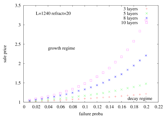
Figure 2: Regime diagram in the sale price versus probability of failure plane. The time lag between bakruptcy and re-birth is 20. Two regions of growth and economical collapse at large times are separated by lines which position are fixed by simulation parameters. We here varied the production network depth: The red ’+’ line was obtained for a 3 layers net, the green ’x’ line for a 5 layers net, the blue ’*’ line for an 8 layers net, and pink square line for a 10 layers net.

Figure 2 displays four breakeven manifolds corresponding to different lattice depths.

At low failure probability, the breakeven lines follow equation 7. At higher values of $\mathcal{P}$, interactions among firms failures are important, hence the non linear increase of compensating prices.

Breakeven manifold are a simple test of the economic performances of the network: when performances are poor, the compensating sales price has to be larger. We checked for instance that increasing the bankruptcy threshold and new firms initial capital increase global economic performance. On the other hand, increasing the time lag between bankruptcy and the apparition of new firms increase breakeven sale prices in the non-linear region.

Among other systematic tests, we checked parent models with more realistic representations of production costs such as:

• Influence of capital inertia; production costs don’t instantly readjust to orders: capital and labour have some inertia which we modeled by writing that productions costs are a maximum function of actual costs and costs at the previous period.

• Influence of the cost of credit: production failures increase credit rates.

Both variants of course yield higher breakeven sale prices; nevertheless these variants display the same generic properties that we will discuss in the next sections.

Most further results, dynamical and statistical, are based on runs close to the breakeven price in order to avoid systematic drifts and recalibrations.

3.3 Time evolution

The simplest way to monitor the evolution of the system is to display the time variations of some of its global performance. Figure 3 displays the time variations of total delivered production $Y^{d}$, total wealth $A$, total undelivered production due to failures and the fraction of active firms for a 1200x10 lattice, with a probability of failure of 0.05 and a compensation sale price of 1.185. Time lag between bankruptcy and and new firm creation is either 1 (for the left diagram) or 5 (for the right digram).

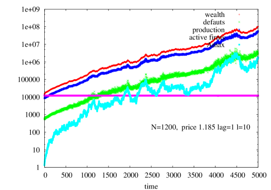
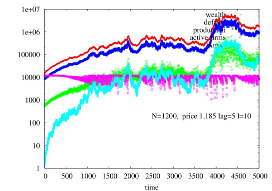
Figure 3: Time evolution of wealth (red ’+’), production (blue ’*’), destroyed production (green ’x’), active firms (magenta empty squares) and production by the largest firm (cyan hollow squares). The network has 10 layers, 200 firms per layer, $\mathcal{P}=0.05$ (the failure probability). The left diagram corresponds to a small time lag (1) between bankruptcy and firm re-birth, right diagram corresponds to a larger time lag (5). Vertical scale is logarithmic, which permits to have the four quantities displayed on the same time plot but reduces the apparent amplitude of fluctuations occurring when time is larger than 1000.

The features that we here report are generic to most simulation at breakeven prices. During the initial steps of the simulation, here say 1000, the wealth distribution widens due to the influences of failures. Bankruptcies cascades do not occur as observed by checking the number of active firms, until the lowest wealth values reach the bankruptcy threshold. All quantities have smooth variations. Later, for $t>1000$ one observes large production and wealth fluctuations characteristic of critical systems.

At larger time lag (5) between bankruptcy and firm re-birth, when bankruptcies become frequent, they can cascade across the lattice and propagate in both network directions as seen on the right diagram of figure 3. A surprising feature of the dynamics is that avalanches of bankruptcies are not correlated with production level. Even when only one tenth of the firms are active, the total production is still high. In fact, in this model, most of the total production is dominated by large firms, and avalanches which concern mostly small firms are of little consequence for the global economy.

Battiston etal study more thoroughly the time dynamics of a related model (large sale price fluctuations possibly inducing bankruptcies and lack of payment) in [11] .

3.4 Wealth and production patterns

Like most reaction-diffusion systems, the dynamics is not uniform in space and display patterns. The wealth and production patterns displayed after 5000 time steps on figure 4 and 5 were obtained for $\mathcal{P}=0.05$ . They reflect wide distributions and spatial organisation. In these diagrams, production flows upward. The upper diagram displays wealth $A$ and the lower one production $Y_{d}$. The intermediate bar is the colour scale, black=0, violet is the maximum wealth or production. (We in fact displayed square roots of $A$ and $Y_{d}$ in order to increase the visual dynamics of the displays; otherwise large regions of the patterns would have been red because of the scale free distributions of $A$ and $Y_{d}$, see further).

The important result is that although production has random fluctuations and diffuses across the lattice, the inherent multiplicative (or autocatalytic) process of production + re-investment coupled with local diffusion results in a strong metastable local organisation: the dynamics clusters rich and productive firms in ”active regions” separated by ”poor regions” (in red or black).

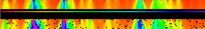
Figure 4: Patterns of wealth(upper pattern) and production (lower pattern) after 5000 iterations steps with the parameter set-up of figure 3 (left) (time lag =1), for a 200x10 lattice. . For both patterns the output layer is the last one above. The intermediate line is the colour code, with minimal amplitude at the extreme left. We observe alternance of highly productive regions (in pink, blue and green colour), with less active regions (in red). Local production failures represented by black dots are randomly distributed across the production pattern. Only one bankrupted firm is observed on the wealth pattern.

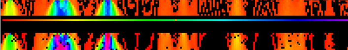
Figure 5: Patterns of wealth(upper pattern) and production (lower pattern) after 5000 iterations steps with the parameter set-up of figure 3 (right) (time lag is 5). The same alternance of active and less active regions is observed, but with a larger time lag (5), we also get large zones of bankrupted firms in black.

Figure 6: Successive patterns of wealth after 250, 750, 1250, 1750 and 2250 time steps with the parameter set-up of figure 3 (right, time lag = 5) for a 1200x10 lattice.

These patterns are evolving in time, but are metastable on a long time scale, say of the order of several 100 time steps as seen on the succession of production patterns at different steps of the simulation as one can observe on figure 6: successive patterns at time 1250, 1750 and 2250.

The relative importance of active (and richer) regions can be checked by a Zipf plot[12]. We first isolate active regions by ”clipping” the dowstream (along $k$ axis) integrated wealth at a level of one thousandth of the total production.

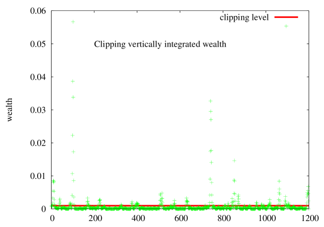
Figure 7: Separating richer regions. Downstream integrated wealth levels (green ’+’) are plotted as a function of their transverse position. The clipping level indicated by the red line isolates richer regions (those wealth peaks above the red line).

We then transversally (along $i$ axis) integrate the wealth of active regions and order these regional wealths to get the Zipf plots.

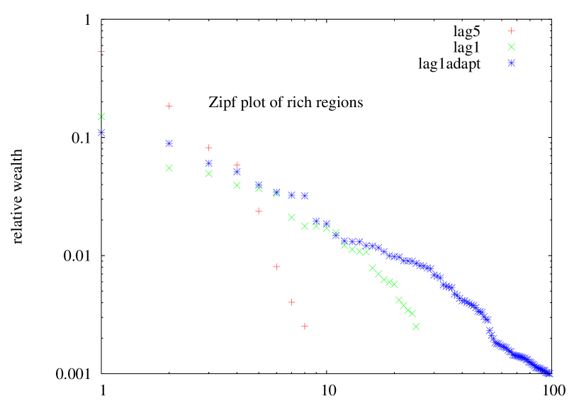
Figure 8: Zipf plot of wealth of the most active regions for the standard and adaptive firms models (cf. section 4.2). The vertical axis display the production relative to the total production. The red ’+’ correspond to the standard model with time lag = 5, green ’x’ to time lag = 1, and blue ’*’ to the adaptive firms model with time lag = 1.

All 3 Zipf plots display some resemblance with standard Zipf[12] plots of individual wealth, firm size and city size. For the model discussed here, the size decrease following approximately a power law. The apparent exponent is one when the time lag is 1. It is much higher when the time lag is 5.

Zipf plots of output active regions (not shown here) display the same characteristics.

When the time lag is 5, the most productive region accounts for more than 50 perc. of total production. The figure is 18 perc. for the second peak. The distribution typically is ”winner takes all”. The equivalent figures when the time lag is 1 are 10 and 8.5 perc..

In conclusion, the patterns clearly display some intermediate scale organisation in active and less active zones: strongly correlated active regions are responsible for most part of the production. The relative importance of these regions obeys a Zipf distribution.

3.5 Wealth and production histograms

The multiplicative random dynamics of capital and the direct observation of wealth and production would lead us to predict a scale free distribution of wealth and production.

The cumulative distribution functions (cdf) of wealth and production observed on figure 8 are indeed wide range and do not display any characteristic scale: The data wealth and production were taken for the same conditions as the previous figures at the end of the simulation, i.e. after 5000 time steps. The medium range of the cdf when time lag is 1 (figure 8a) extends on one and a half decade with an apparent slope of $1\pm 0.05$ in log-log scale.

This observed dependence of the wealth cdf, log normal at lower $A$ values followed by power law at intermediate $A$ values, is consistent with expressions derived for pdf in the literature on coupled differential equations with multiplicative noise. Bouchaud and Mézard[14] e.g. obtained:

$$P(w)=Z\frac{exp-\frac{1-\mu}{w}}{w^{1+\mu}}$$ (8)

(where $w$ stands for the wealth relative to average wealth $\bar{A}$), from the differential system:

$$\frac{dA_{i}}{dt}=\eta_{i}(t)\cdot A_{i}+J\cdot(\bar{A}-A_{i}).$$ (9)

where $\eta_{i}(t)$ is a random multiplicative noise, with variance $\sigma^{2}$; $\mu=1+\frac{J}{\sigma^{2}}$.

At higher wealth, the straight line giggles and drops much faster: this is because of the underlying region structure. The last 80 perc. of the wealth is concentrated in two rich regions and its distribution is dominated by local diffusion phenomena in these regions.

The departure form the standard (equ.8) distribution is even more noticeable when avalanches are present. The large wealth shoulder is bigger (95 perc. of production) and the first point at zero wealth stands well above the rest of the distribution: it corresponds to those 50 perc. of the firms which are momentarily bankrupted. The fraction of bankrupted firms fluctuates in time and so does the slope of the linear segment.

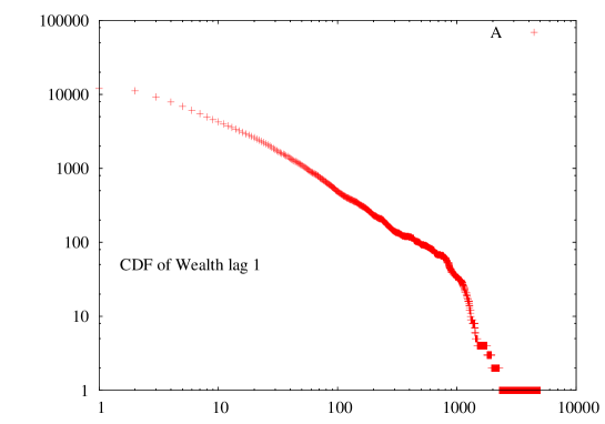
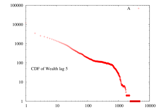
Figure 9: Cumulative distribution of wealth (red ’+’) after 5000 iteration steps. Parameter choices are the same as the previous figures.

In conclusion, the observed statistics largely reflect the underlying region structure: at intermediate levels of wealth, the different wealth peaks overlap (in wealth, not in space!): we then observed a smooth cdf obeying equation 8. At the large wealth extreme the fine structure of peaks is revealed.

4 Conclusions

The simple model of production networks that we proposed presents some remarkable properties:

• Scale free distributions of wealth and production.

• Large spatial distribution of wealth and production.

• A few active regions are responsible for most production.

• Avalanches of bankruptcies occur for larger values of the time lag between bankruptcy and firm re-birth. But even when most firms are bankrupted, the global economy is little perturbed.

Are these properties generic to a large class of models? we will first briefly report on equations which display similar behaviour and then examine the results which we obtained with variants of the model.

4.1 Formal approaches of similar dynamics

A number of models which display equivalent phenomena have been proposed and formally solved. We kept our own notation to display similarities:

• Growth by deposition on surfaces[15], Edwards/Wilkinson:

  $$\frac{dA}{dt}=D\cdot\Delta A+\eta(x,t)$$ (10)

  $A$ stands for the distance to the interface. $D$ is the surface diffusion constant of the deposited material and $\eta_{i}(t)$ is an addititive noise. Other models were proposed by Karkar/Parisi/Zhang, Derrida/Spohn[15], etc.

• Generalised Volterra-Lotka from econophysics: (Bouchaud[14], Cont, Mezard, Sornette, Solomon[16] etc.)

  $$\frac{dA_{i}}{dt}=A_{i}\cdot\eta_{i}(t)+\sum_{j}J_{ij}A_{j}-\sum_{j}J_{ji}A_{i}$$ (11)

  $A$ stands for individual wealth of agents and $\eta_{i}(t)$ is a multiplicative noise. Agents are involved in binary transactions of ”intensity” $J_{ij}$. Mean field formal solutions displays scale free distribution of wealth. Simulations display patterns on lattice structures (Souma etal[17]).

• Solomon etal[18]. Reaction-Diffusion AB models.

  $$\frac{dA}{dt}=k\cdot A\cdot\eta(x,t)+D\cdot\Delta A$$ (12)

  $A$ is the chemical concentration of a product involved in an auto-catalytic chemical reaction, $D$ is its diffusion constant. Simulations and formal derivations yield spatio-temporal patterns similar to ours.

4.2 Variants of the original model

We started checking three variants, with for instance more realistic production costs taking into account:

• Influence of capital inertia: production costs don’t instantly readjust to orders; capital and labour have some inertia which we modeled by writing that productions costs are a maximum function of actual costs and costs at the previous period.

• Influence of the cost of credit: production failures increase credit rates.

The preliminary simulations confirm the genericity of our results.

The third variant is a model with ”adaptive firms”. The lattice connection structure supposes a passive reactive behaviour of firms. But if a firm is consistently delivering less than the orders it receives, its customers should order less from it and look for alternative suppliers. Such adaptive behaviour leading to an evolutive connection structure would be more realistic.

We then also checked an adaptive version of the model by writing that orders of firm $i$ are proportional to the production capacity $A$ of the upstream firms connected to firm $i$. Simulations gave qualitative results similar to those obtained with fixed structures.

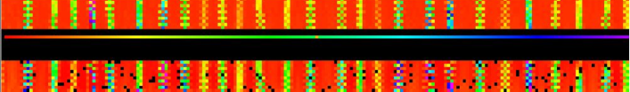
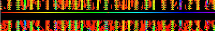
Figure 10: Wealth and production patterns for a network of ”adaptive” firms. The conventions and parameters are the same as for figures 3, 4 and 5, for a 200x10 lattice. Time lag is 1, the two upper patterns correspond to $t=1500$, the lower ones were taken when $t=1998$.

We observe that adaptation strongly re-enforce the local structure of the economy. The general picture is the same scale free distribution of production and wealth with metastable patterns. Due to the strong local character of the economy:

• Avalanches of production are observed (see figure 9), even when time lag is short (time lag of 1).

• The spatial periodicity of the active zones is increased (see figure 9 with larger density of smaller zones). But again the activity distribution among zones is like ”winner takes all” (figure 7).

4.3 Checking stylised facts

Even though the present model is quite primitive it is still tempting to draw some conclusions that could apply to real economies. The most striking result to our mind is the strong and relatively stable spatial disparities that it yields. Let us compare this prediction to the economic situation of developing countries: large and persistent disparities in wealth and production level as compared to developed countries. We can even go further and raise questions about the influence of the depth of the production network or the kind of investment needed:

• One generally agrees that disparities between developing and developed countries increased since industrial revolution. This is also a period during which production became more specialised, which translates in our model as increasing the network depth: for instance a shoemaker would in the past make and sell a pair of shoes from leather obtained from a cattle breeder. Nowadays the shoe production and delivery process involve many more stages. Our simulations have shown that increasing depth increases the fragility of economies to failures and bankruptcies. The new industrial organisation may have detrimental effects on developing economies.

• Obviously investment policies in developing countries yield some coordination across the whole production chain. Bad economic results might be due to very local conditions but can also reflect the lack of suppliers/producers connections.

The above remarks are not counter-intuitive and these conclusions could have been reached by verbal analysis. What is brought by the model is the dramatic and persistent consequences of such apparently trivial details.

Acknowledgments: We thank Bernard Derrida and Sorin Solomon for illuminating discussions and the participants to CHIEF Ancona Thematic Institute, especially Mauro Gallegati. CHIEF was supported by EXYSTENCE network of excellence, EC grant FET IST-2001-32802. This research was also supported by COSIN FET IST-2001-33555, E2C2 NEST 012975 and CO3 NEST 012410 EC grants.

References

- [1] D. J. Watts and S. H. Strogatz, Collective dynamics of small-world networks, Nature 393, 440 442 (1998).
- [2] R. Albert and A.L. Barabási, Rev. Mod. Phys. 74,(2002), 47.
- [3] Davis, G.F. and Greve, H.R., Corporate elite networks and governance changes in the 1980s, Am. J. of Sociology, 103, 1-37 (1996).
- [4] Battiston, S., Bonabeau, E., Weisbuch G., Decision making dynamics in corporate boards, Physica A, 322, 567 (2003).
- [5] Battiston, S., Weisbuch G., Bonabeau, E., Decision spread in the corporate board network, 2003, to appear on Adv.Compl.Syst.
- [6] ”Battiston, S., Caldarelli G., Garlaschelli D., The hidden topology of shareholding networks, 2003, submitted.
- [7] “Towards a New Paradigm in Monetary Economics” (Raffaele Mattioli Lectures) by Joseph Stiglitz, Bruce Greenwald, Cambridge ch 7
- [8] ”A new approach to business fluctuations: heterogeneus interacting agents, scaling laws and financial fragility” D. Delli Gatti, C. Di Guilmi, E. Gaffeo, G. Giulioni, M. Gallegati and A. Palestrini, Journal of Economic Behavior & Organization, 2004.
- [9] Powell, W. W.; Koput, K. W.; Smith-Doerr, L. ”Interorganizational Collaboration and the Locus of Innovation: Networks of Learning in Biotechnology. ” Administrative Science Quarterly, 1996, Vol. 41 Issue 1, p116,
- [10] Bak P., Chen K., Scheinkman J. and M. Woodford (1993), ”Aggregate Fluctuations from Independent Sectoral Shocks: Self-Organized Criticality in a Model of Production and Inventory Dynamics”, Ricerche Economiche, 47:3-30.
- [11] Battiston S., Delli Gatti D., Gallegati M., Greenwald B., Stiglitz J.E.,(2005) ”Credit Chains and Bankruptcies Avalanches in Supply Networks”, submitted.
- [12] Zipf, G.K., 1949. ”Human behavior and the principle of least effort” -Hafner. Benoit B. Mandelbrot 1951. ”Adaptation d’un message sur la ligne de transmission. I Quanta d’information.”, Comptes rendus (Paris): 232, 1638-1740.
- [13] Kesten, H. (1973) ”Random difference equations and renewal theory for products of random matrices”. Acta Math. 131, pp. 207-248.
- [14] JP Bouchaud, M Mezard ”Wealth condensation in a simple model of economy” Arxiv preprint cond-mat/0002374, 2000 - arxiv.org
- [15] T. Halpin-Healey and Y.-C. Zhang, Phys. Rep. 254, 215 (1995). M. Kardar, G. Parisi, and Y.-C. Zhang, Phys. Rev. Lett. 56 (1986), 889. B Derrida, H Spohn, ”Polymers on disordered trees, spin glasses, and traveling waves” J. Stat. Phys, 51, P. 817, (1988).
- [16] Solomon, S. Generalized Lotka-Volterra (GLV) Models http://xxx.lanl.gov/pdf/cond-mat/9901250 in Applications of simulation to social sciences, Ballot and Weisbuch ed., Hermes, Paris (2000). D Sornette, R Cont, ”Convergent multiplicative processes repelled from zero: power laws and truncated power laws” Arxiv preprint cond-mat/9609074, 1996 - arxiv.org .
- [17] W Souma, Y Fujiwara, H Aoyama ”Small-World Effects in Wealth Distribution” Arxiv preprint cond-mat/0108482, 2001 - arxiv.org
- [18] Shnerb N. M., Louzoun Y.,Bettelheim E., Solomon S. (1999) ”The importance of being discrete - life always wins on the surface” http://xxx.lanl.gov/pdf/adap-org/9912005