Criterion for traffic phases in single vehicle data and empirical test of a microscopic three-phase traffic theory

Abstract

A microscopic criterion for distinguishing synchronized flow and wide moving jam phases in single vehicle data measured at a single freeway location is presented. Empirical local congested traffic states in single vehicle data measured on different days are classified into synchronized flow states and states consisting of synchronized flow and wide moving jam(s). Then empirical microscopic characteristics for these different local congested traffic states are studied. Using these characteristics and empirical spatiotemporal macroscopic traffic phenomena, an empirical test of a microscopic three-phase traffic flow theory is performed. In accordance with real traffic, a model of an $``$open” road is applied; traffic demand at model boundaries is taken from empirical data. Spatiotemporal congested model patterns emerge, develop, and dissolve due to self-organization effects. In accordance with the microscopic criterion for the traffic phases, the synchronized flow and wide moving jam phases are found in single vehicle model data associated with different locations within the spatiotemporal congested model patterns. Simulations show that the microscopic criterion and macroscopic spatiotemporal objective criteria lead to the same identification of the synchronized flow and wide moving jam phases in congested traffic. It is found that microscopic three-phase traffic models can explain both microscopic and macroscopic empirical congested pattern features. It is obtained that microscopic frequency distributions for vehicle speed difference as well as fundamental diagrams and speed correlation functions can depend on the spatial co-ordinate considerably. It turns out that microscopic optimal velocity (OV) functions and time headway distributions are not necessarily qualitatively different, even if local congested traffic states are qualitatively different. The reason for this is that important spatiotemporal features of congested traffic patterns are lost in these as well as in many other macroscopic and microscopic traffic characteristics, which are widely used as the empirical basis for a test of traffic flow models, specifically, cellular automata traffic flow models.

I Introduction

Freeway traffic is a complex dynamic process, which unfolds in space and time. Specifically, in initial free flow complex spatiotemporal congested patterns are observed. Therefore, for an adequate comparison with reality a model should exhibit features of the onset of congestion and of empirical spatiotemporal congested traffic patterns. To observe these patterns, measurements of traffic variables (e.g., flow rate and vehicle speed) as functions of time at many different freeway locations should simultaneously be made on a long enough freeway section. From spatiotemporal analysis of such data measured over many days and years on various freeways in different countries, it has been found that there are two different phases in congested traffic, synchronized flow and wide moving jam (see references in the book KernerBook ). Thus, there are three-traffic phases: 1. Free flow. 2. Synchronized flow. 3. Wide moving jam.

The fundamental difference between synchronized flow and wide moving jam is determined by the following macroscopic spatiotemporal objective (empirical) criteria KernerBook . The wide moving jam exhibits the characteristic, i.e., unique, and coherent feature to maintain the mean velocity of the downstream jam front, even when the jam propagates through any other traffic states or freeway bottlenecks. In contrast, synchronized flow does not exhibit this characteristic feature, in particular, the downstream front of synchronized flow is often fixed at a freeway bottleneck.

Congested traffic occurs mostly at freeway bottlenecks. Just as defects and impurities are important for phase transitions in physical systems, so are bottlenecks in traffic flow. In empirical observations, the following fundamental spatiotemporal features of phase transitions and congested patterns have been found KernerBook :

(1) The onset of congestion at a bottleneck is associated with a local phase transition from free flow to synchronized flow. This F$\rightarrow$S transition exhibits probabilistic nature. In particular, the F$\rightarrow$S transition can be induced by a short-time disturbance that plays the role of a critical nuclei for the phase transition.

(2) There can be spontaneous and induced F$\rightarrow$S transitions at a freeway bottleneck.

(3) Wide moving jams can emerge spontaneously only in synchronized flow, i.e., due to F$\rightarrow$S$\rightarrow$J transitions.

(4) There are two main types of congested patterns at an isolated bottleneck: A synchronized flow pattern (SP) and a general pattern (GP). An SP consists of synchronized flow only, i.e., no wide moving jams emerge in the SP. An GP is a congested pattern, which consists of synchronized flow upstream of the bottleneck and wide moving jams that emerge spontaneously in this synchronized flow.

To explain the complex dynamic process of freeway traffic, a huge number of traffic flow models have been introduced. The last few years have seen a rapid development of traffic flow physics in relation to new modeling approaches (see the reviews Gartner ; Wolf ; Sch ; Helbing2001 ; Nagatani_R ; Nagel2003A ; MahnkeRev , the book KernerBook , and the conference proceedings Lesort ; Ceder ; Taylor ; SW1 ; SW2 ; SW3 ; SW4 ; SW5 ).

Past traffic flow theories and models reviewed in Gartner ; Wolf ; Sch ; Helbing2001 ; Nagatani_R ; Nagel2003A cannot explain and predict the spatiotemporal features of traffic mentioned in item (1)–(4) above. The only one exception is the characteristic features of wide moving jam propagation that can be shown in some of these models KernerBook . To explain empirical results of item (1)–(4), Kerner introduced three-phase traffic theory Kerner1998B ; Kerner2002B . The hypotheses of this theory are the basis of a microscopic three-phase traffic theory KKl ; KKW ; KKl2003A ; KKl2004AA . Recently, some new microscopic models in the context of three-phase traffic theory have been suggested Davis2003B ; Lee_Sch2004A ; Jiang2004A .

Microscopic three-phase traffic theory of Ref. KKl ; KKW ; KKl2003A ; KKl2004AA can explain macroscopic spatiotemporal congested pattern phenomena KernerBook . Macroscopic traffic flow characteristics can depend strongly on the pattern type and on the freeway location within the pattern. Thus, we can expect that this conclusion is also valid for single vehicle (i.e., microscopic) traffic flow characteristics. However, single vehicle data measured at many different freeway locations, which can be sufficient for a reliable spatiotemporal analysis of the whole congested pattern structure, are not available up to now.

In this paper, a microscopic empirical criterion for the synchronized flow and wide moving jam phases in congested traffic is found. This criterion enables us to distinguish the phases in empirical single vehicle data measured at a single freeway location, i.e., even without a spatiotemporal congested pattern analysis required for application of the macroscopic spatiotemporal objective criteria for the traffic phases. Based on the associated empirical single vehicle data analysis, an empirical test of a microscopic three-phase traffic theory of Ref. KKl ; KKW ; KKl2003A ; KKl2004AA is performed.

The article is organized as follows. Empirical findings are considered in Sect. II. Firstly, a microscopic empirical criterion for the phases in congested traffic is suggested and used for an empirical single vehicle data analysis (Sect. II.2). Based on this analysis, empirical microscopic characteristics of local congested states are found (Sect. II.3). Finally, some of the fundamental empirical macroscopic spatiotemporal pattern features are briefly discussed (Sect. II.4). In Sect. III, microscopic and macroscopic congested model patterns and their characteristics are compared with empirical results. Firstly, model spatiotemporal congested pattern evolution under time-dependence of traffic demand taken from empirical results is studied and compared with the empirical macroscopic spatiotemporal patterns of Sect. II.4. Then these spatiotemporal congested patterns are used to find model microscopic characteristics from single vehicle data associated with different locations within the patterns. Finally, a proof of the microscopic criterion for the phases in congested traffic as well as a comparison of empirical and microscopic traffic model characteristics are presented.

II Empirical Results

II.1 Congested States in Single Vehicle Data

Single vehicle characteristics are usually obtained either in driver experiments or through the use of detectors (e.g., Neubert ; Knospe2002 ; Knospe2004 ; Cowan ; Koshi ; Luttinen ; Bovy ; Tilch2000 ; Banks ; Gurusinghe2003A ). In the latter case, data from a single freeway location or aggregated data measured at different locations are used Aggregated . For empirical tests of traffic flow models time headway distributions (probability density for different time headways) and optimal velocity (OV) functions (the mean speed as a function of space gap between vehicles at a given density) are often used (e.g., Knospe2004 ).

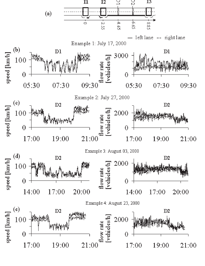
Figure 1: Macroscopic characteristics of empirical single vehicle data: (a) – Sketch of detector arrangement. (b) – Local traffic dynamics (one-minute average data) of the speed (left) and flow rate (right) on four different days in both freeway lanes.

Single vehicle data have been measured from June 01, 2000 till September, 30, 2000 on a two-lane section of the freeway A92-West with two sets of double induction loop detectors (D1 and D2) between intersections $``$AS Freising Süd” (I2) and $``$AK Neufahm” (I3) near Münich Airport in Germany (intersection I1: $``$AS Flughafen” in Fig.  1 (a)). Each detector set consists of two detectors for the left (passing) and right lanes. A detector registers a vehicle by producing a current electric pulse whose duration $\Delta t_{i}$ is related to the time taken by the vehicle to traverse the induction loop. This enables us to calculate the gross time gap between two vehicles $i$ and $i+1$ that have passed the loop one after the other $\tau^{\rm(gross)}_{i,i+1}$. There are two detector loops in each detector. The distance between these loops is constant. This enables us to calculate the individual vehicle speed $v_{i}$, the vehicle length $d_{i}=v_{i}\Delta t_{i}$, as well as the net time gap (time headway) between the vehicles $i$ and $i+1$: $\tau_{i,i+1}=\tau^{\rm(gross)}_{i,i+1}-\Delta t_{i}$.

Local dynamics of the average speed and flow rate (one-minute average data) for four typical days at which congested traffic have been observed are shown in Fig.  1 (b). The local congested traffic dynamics from July 17, 2000 is designated below as $``$example 1”, whereas the dynamics from July 27, August 03, and 27, 2000 are designated as $``$examples 2–4”, respectively.

From consideration of the flow rate for the examples 1–4, it can be seen that even if within the local dynamics for the examples 2–4 there are moving jams, then these jams should mostly be narrow moving jams, i.e., these examples should correspond to the synchronized flow phase. Indeed, there are no drops in the flow rate, which are typical for wide moving jams KernerBook , during the whole time of congested traffic existence in the examples 2–4. In contrast, in the example 1 there are short-time drops both in the average speed and flow rate within the local congested dynamics (example 1, left in Fig.  1 (b)). Such drops are usually typical for wide moving jams MovingJams . However, from these macroscopic data (example 1, Fig.  1 (b)) measured at a single location only we cannot make a conclusion with certainty whether these drops are associated with the wide moving jam phase or not. Nevertheless, this conclusion can be made, if a microscopic criterion for the traffic phases presented below is applied.

II.2 Traffic Flow Interruption Effect as Microscopic Criterion for Wide Moving Jam

The characteristic wide moving jam feature to propagate through a bottleneck while maintaining the downstream jam velocity, which distinguishes the wide moving jam from synchronized flow (in accordance with the macroscopic spatiotemporal objective criteria for the traffic phases in congested traffic), can be explained by a traffic flow discontinuity within a wide moving jam. Traffic flow is interrupted by the wide moving jam: There is no influence of the inflow into the jam on the jam outflow. For this reason, the mean downstream jam front velocity and the jam outflow exhibit fundamental characteristic features, which do not depend on the jam inflow KernerBook . A difference between the jam inflow and the jam outflow changes the jam width only. This traffic flow interruption effect is a general effect for each wide moving jam.

The jam outflow becomes independent of the jam inflow, when the traffic flow interruption effect within a moving jam occurs. This is realized, when due to a very low vehicle speed or a vehicle standstill the maximum gross time headway $\tau^{\rm(gross)}_{\rm max}$ between two vehicles within the jam is considerably longer than the mean time delay $\tau^{\rm(ac)}_{\rm del}$ in vehicle acceleration at the downstream jam front from a standstill state LongVehicles :

$$\tau^{\rm(gross)}_{\rm max}\gg\tau^{\rm(ac)}_{\rm del}.$$ (1)

Indeed, the time delay $\tau^{\rm(ac)}_{\rm del}$ determines the jam outflow TimeDelay . Under the condition (1), there are at least several vehicles within the jam that are in a standstill or if they are still moving, it is only with a negligible low speed in comparison with the speed in the jam inflow and outflow. These vehicles separate vehicles accelerating at the downstream jam front from vehicles decelerating at the upstream jam front: The inflow into the jam has no influence on the jam outflow. Then the jam outflow is fully determined by vehicles accelerating at the downstream jam front. As a result, the mean downstream jam front velocity is equal to $v_{\rm g}=-1/(\tau^{\rm(ac)}_{\rm del}\rho_{\rm max})$ KernerBook ($\rho_{\rm max}$ is the density within the jam) regardless of whether there are bottlenecks or other complex traffic states on the freeway. In other words, this jam propagates through a bottleneck while maintaining the mean downstream jam front velocity $v_{\rm g}$, i.e., in accordance with the macroscopic objective spatiotemporal criteria for the traffic phases in congested traffic (Sect. I) this jam is a wide moving jam.

Thus, the traffic flow interruption effect can be used as a criterion to distinguish between the synchronized flow and wide moving jam phases in single vehicle data. This is possible even if data is measured at a single freeway location. This enables us to find dependence of single vehicle characteristics on different local microscopic congested pattern features (Sect. II.3).

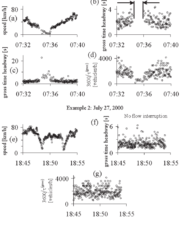
Figure 2: Microscopic criterion for wide moving jam: (a–d) – Empirical single vehicle data for speed within a wide moving jam in the left lane (a) and the associated time distributions of gross time headways $\tau^{\rm(gross)}$ for different scales of the time headways (b, c) and of the value $3600/\tau^{\rm(gross)}$ (d) related to the example 1 in Fig. 1 (b). (e–g) – Empirical single vehicle data for speed within a sequence of two narrow moving jams in the left lane (e) and the associated time distributions of $\tau^{\rm(gross)}$ (f) and of $3600/\tau^{\rm(gross)}$ (g) related to the example 2 in Fig. 1 (b).

The interruption of traffic flow within a moving jam shown in Fig. 2 (a) is clearly seen in the time-dependences of gross time headways $\tau^{\rm(gross)}$ (Fig. 2 (b, c)) and of the value $3600/\tau^{\rm(gross)}$ (Fig. 2 (d)). Before and after the jam has passed the detector D1 (due to the jam upstream propagation MovingJams ) there are many vehicles that traverse the induction loop of the detector. Within the jam, there are no vehicles traversing the detector with synchronized flow gross time headways $<4$ sec during a time interval (this time interval is labeled $``$flow interruption” in Fig. 2 (b)), when the speed within the jam is approximately zero (Fig. 2 (a)). This means that traffic flow is discontinuous within the moving jam, i.e., this moving jam is associated with the wide moving jam phase. If all gross time headways for the time interval are considered (Fig. 2 (c)), then it can be seen that the $``$real” duration of flow interruption within the wide moving jam, i.e., when vehicles do not move through the detector at all, is equal to approximately 20 sec: There is a vehicle with the gross time headway $\approx$ 20 sec. Later, some vehicles, which are within the jam, exhibit gross time headways about 5 sec or longer. The latter can be explained by moving blanks within the jam (see Sect.11.2.4 in KernerBook ). This is correlated with the result that only after the jam (at $t>$ 7:36) has passed the detector, synchronized flow gross time headways (1–4 sec) are observed (Fig. 2 (c)). Similar results are found for other moving jams in single vehicle data.

In examples 2–4 (Fig.  1 (b)), there also are many moving jams during the time intervals of congested traffic. For example, the speed within two moving jams in Fig. 2 (e) (the example 2) is also very low. Nevertheless, in contrast with the wide moving jam in Fig. 2 (a) rather than wide moving jams these moving jams should be classified as narrow moving jams KernerBook . This is because there are no traffic flow interruptions within these moving jams (Fig. 2 (f, g)). Indeed, upstream, downstream of the jams, and within the jams there are many vehicles that traverse the induction loop of the detector: There is no qualitative difference in the time-dependences of gross time headways for different time intervals associated with these narrow jams and in traffic flow upstream or downstream of the jams (Fig. 2 (f)).

This can be explained if it is assumed that each vehicle, which meets a narrow moving jam, must decelerate down to a very low speed within the jam, can nevertheless accelerate later almost without any time delay within the jam: The narrow moving jam consists of upstream and downstream jam fronts only. Within the upstream front vehicles must decelerate. However, they then can accelerate almost immediately at the downstream jam front. These assumptions are confirmed by single vehicle data shown in Fig. 2 (f, g), in which time intervals between different measurements of gross time headways and for the value $3600/\tau^{\rm(gross)}$ for different vehicles exhibit the same behavior away and within the jams. Thus, regardless of these narrow moving jams traffic flow is not discontinuous, i.e., the narrow moving jams belong indeed to the synchronized flow traffic phase.

This single vehicle analysis enables us to conclude that congested traffic in the example 1 is associated with a sequence of wide moving jams propagating in synchronized flow. In contrast, congested traffic in the examples 2–4 is mostly associated with different states of the synchronized flow phase.

II.3 Dependence of Single Vehicle Characteristics on Local Congested Pattern Features

II.3.1 Time Headway Distributions

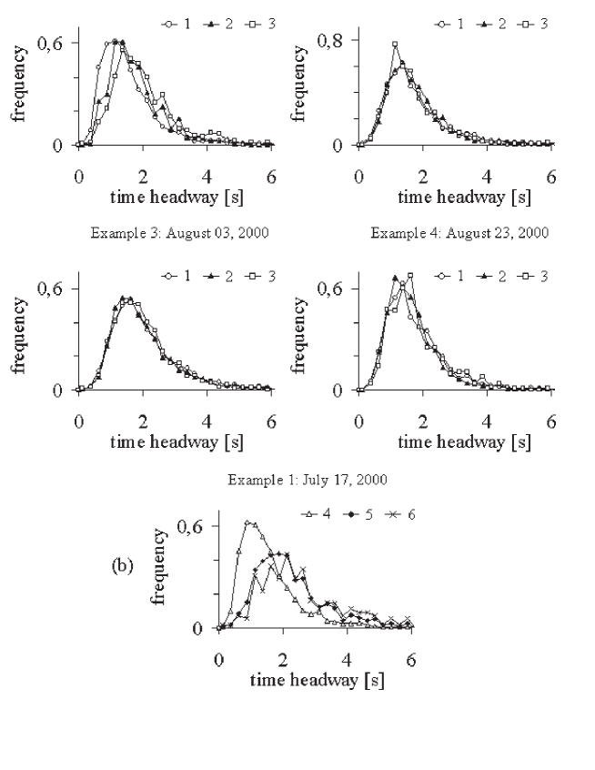
Figure 3: Empirical time headway distributions: (a) – For the examples 1–4 in Fig. 1 (b) for different density ranges: curve 1 – 20 $<\rho<$ 30, curve 2 – 30 $<\rho<$ 40, curve 3 – 40 $<\rho<$ 50 vehicles/km. (b) – Time headway distributions associated with the example 1 for different speed ranges: curve 4 – $v>$ 50, curve 5 – $v<$ 30, curve 6 – $v<$ 20 km/h. Left lane.

Although local traffic dynamics in the example 1 is qualitatively different from the examples 2–4, the related time headway distributions found for different density ranges are qualitatively the same (Fig. 3 (a)). Moreover, the distributions are both qualitatively and even approximately quantitatively the same as those found for congested traffic on different freeways in various countries (e.g. Bovy ; Neubert ; Tilch2000 ; Knospe2002 ). Thus, based only on these time headway distributions it is not possible to distinguish different synchronized flow local dynamics in the examples 2–4 one from another and also from the example 1 with wide moving jams.

However, the time headway distributions for the example 1 with wide moving jams exhibit some peculiarities: If time headway distributions for vehicles whose speed $v>$ 50 km/h, $v<$ 30 km/h, and $v<$ 20 km/h are drawn separately, then it turns out that the lower the speed, the more shifted become the time headway distributions to longer time headways (Fig. 3 (b)). As should be expected, the time headway distributions for the vehicles away from the jams (with $v>$ 50 km/h) are almost the same as those for synchronized flow without a wide moving jam sequence (examples 2–4). In contrast, vehicles within wide moving jams exhibit appreciable longer time headways, which are the longer, the lower the speed. As a data analysis shows, these time headways are mostly associated with moving blanks within the jams. However, even these differences in the time headway distributions say nothing about jam duration, speed distributions between the jams, and many other spatiotemporal congested traffic characteristics.

We can conclude that the microscopic characteristic of congested traffic $``$time headway distribution” cannot be used for clear distinguishing spatiotemporal congested pattern features. This is because within time headway distributions most of spatiotemporal traffic characteristics are averaged. Because the sum of wide moving jam duration in the example 1 is shorter than the synchronized flow duration, it is almost impossible to distinguish much longer time headways associated with moving blanks within the jams. Only when the share of the jams in the time headway distribution increases (Fig. 3 (b), $v<$ 20 km/h), the effect of moving blanks can be identified.

II.3.2 Optimal Velocity (OV) Functions

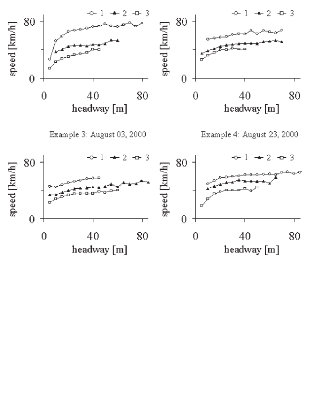
Figure 4: Empirical OV functions for the examples 1–4 in Fig. 1 (b) for different density ranges: Curves 1 – $20<\rho<30$, curves 2 – $30<\rho<40$, curves 3 – $40<\rho<50$ vehicles/km. Left lane.

OV functions are space gap (headway) dependencies of the mean vehicle speed calculated for different given density ranges Neubert . The OV functions found do not exhibit some qualitative differences for the different examples 1–4 of local congested traffic dynamics (Fig. 4). They are qualitatively the same as the OV functions first derived for aggregated single vehicle data in Neubert : At smaller headways the speed increases with headways considerably, whereas for larger headways there is a saturation effect for the speed growth.

We can conclude that microscopic OV functions cannot also be used for clear distinguishing spatiotemporal congested pattern features. This is because within OV functions many of the spatiotemporal traffic characteristics are averaged.

II.4 Spatiotemporal Macroscopic Congested Patterns

In Sects. II.4 and II.5, a brief discussion of empirical macroscopic spatiotemporal traffic features considered in Kerner2002B ; KernerBook is made that is necessary for the empirical test of a microscopic three-phase traffic theory.

Results of empirical investigations reviewed in the book KernerBook enable us to conclude that there are a huge number of different congested traffic patterns, whose spatiotemporal structure depends on type, feature, and location of a freeway bottleneck(s), on other peculiarities of a freeway network, as well as on traffic demand, weather, and other traffic conditions. At first glance all these look like very different patterns, however, it turns out they exhibit clear common features and characteristics KernerBook . Empirical investigations of data measured over many days and years on freeways in various countries show that common traffic phenomena and characteristics of congested patterns, which are most frequent observed, are as follows. (i) GP emergence and evolution that occur at an on-ramp bottleneck (Sect. II.4.1). (ii) Complex congested pattern emergence and transformation that occur at two adjacent off- and on-ramp bottlenecks (Sect. II.4.2).

II.4.1 General Pattern at On-Ramp Bottleneck

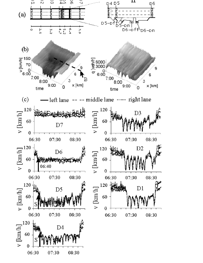
Figure 5: GP upstream of the bottleneck at the effectual on-ramp D6 on a section of the freeway A5-South: (a) – Sketch of the freeway section (left) with detector arrangement within the intersection $I1$ (right). (b) – Vehicle speed averaged across all lanes (left) and total flow rate across the freeway (right) in space and time. (c) – Vehicle speed in different freeway lanes within the GP at different detectors. Data from April 15, 1996. Explanation of the section and the on-ramp bottleneck at D6 see in KernerBook .

In Fig. 5, general pattern (GP) formation at an on-ramp bottleneck is shown KernerBook . Firstly, an F$\rightarrow$S transition occurs at the bottleneck (up-arrow at detector D6). Synchronized flow propagates upstream (up-arrows $S$ at detectors D5–D4), whereas free flow remains downstream (detector D7): The downstream front of synchronized flow is fixed at the bottleneck.

Upstream of the bottleneck the pinch effect in synchronized flow is realized: The speed decreases (detector D5) and density increases. Narrow moving jams emerge spontaneously in the pinch region in synchronized flow (detectors D5–D4). These jams propagate upstream. Some of the jams transform into wide moving jams: The region of wide moving jams propagating upstream is formed (detectors D3–D1).

II.4.2 Complex Pattern Emergence and Transformation on Freeways with two Different Adjacent Bottlenecks

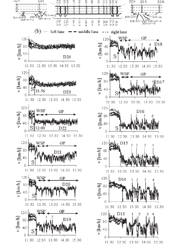
Figure 6: Congested pattern evolution on a section on the freeway A5-North with off-ramp (at D25-off) and on-ramp (at D16) bottlenecks: (a) – Sketch of the section (middle) with detector arrangement within the intersection $I3$ (left) and $I4$ (right). (b) – Vehicle speed over time shown at different detectors. Explanation of the section and the on-ramp and off-ramp bottlenecks see in KernerBook .

Characteristic features of complex pattern emergence and transformation are often observed at a freeway section with two adjacent bottlenecks: An off-ramp bottleneck that is downstream and an on-ramp bottleneck that is upstream KernerBook . In the example in Fig. 6, firstly a widening SP (WSP) at the off-ramp bottleneck emerges. Moreover, an expanded pattern (EP) appears, in which synchronized flow affects both bottlenecks. The EP appears after synchronized flow of the initial WSP covers the on-ramp bottleneck. Secondly, the WSP transforms into an GP at the off-ramp bottleneck.

After the synchronized flow covers the on-ramp bottleneck, wide moving jams begin to emerge downstream of the on-ramp bottleneck within the initial WSP: Rather than the WSP remaining, an GP appears at the off-ramp bottleneck, i.e., congestion emergence at the upstream bottleneck leads to intensification of congestion at the downstream bottleneck. Wide moving jams (labeled 1–4 in Fig. 6 (b)) that emerge within the GP, i.e., between the off-ramp and on-ramp bottlenecks, propagate through the on-ramp bottleneck while maintaining the mean velocity of the jam downstream front.

II.5 Spatial Dependence of Empirical Macroscopic Traffic Flow Characteristics

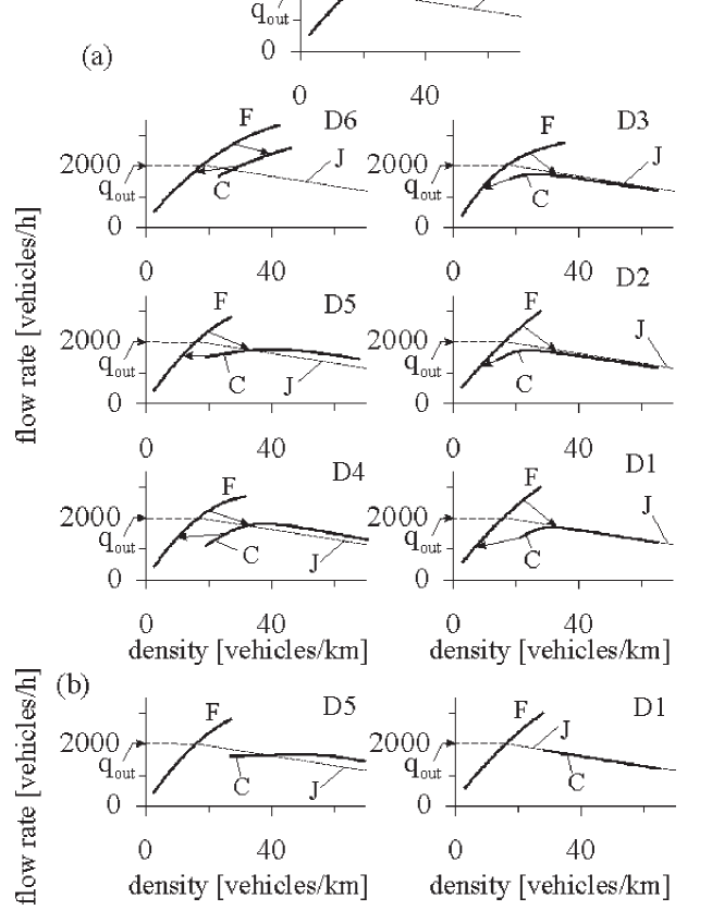
Figure 7: Empirical fundamental diagram at different freeway locations for the left freeway lane related to the GP in Fig. 5: (a) – All data is used KernerBook . (b) – Only data before 8:00 is used. Dotted line shows the line $J$, which represents the upstream propagation of the wide moving jam downstream front; $q_{\rm out}$ is the flow rate in free flow formed by the wide moving jam outflow.

Because a qualitative behavior of the congested traffic dynamics strongly depends on a chosen detector location within a pattern, local pattern characteristics are functions on the spatial co-ordinate. In particular, the fundamental diagram depends both on the pattern type and on a location within a congested pattern at which the flow rate and speed are measured. The fundamental diagram consists of the branches for free flow (curves $F$) and congested traffic (curves $C$ in Fig. 7).

In the case of the GP at the on-ramp bottleneck (Fig. 5 (b, c)), at the locations D6 and D5 the braches $C$ for congested traffic are associated with synchronized flow only. In synchronized flow at D6, the branch $C$ has a positive slope in the flow–density plane. This behavior is changed for the pinch region of synchronized flow (D5). Due to narrow moving jam emergence in the pinch region at greater densities the branch $C$ has a slightly negative slope, whereas at smaller densities of synchronized flow it has a slightly positive slope, i.e., there is a maximum on the branch $C$. However, this maximum is very weak: The flow rate does not approximately depend on density within the pinch region of the GP.

This is explained in Fig. 7 (b), in which empirical data from the time interval 06:45—8:00 of the strong congestion condition are used only. In this case, in the pinch region (at D5) the part on the curve $C$ with the positive slope disappears and the flow rate is almost independent on density (only at greater density there is a slight decrease in flow rate due to narrow moving jam emergence in the pinch region). This also means that the part of the curve $C$ with the positive slope at D5 is associated with the time interval after 8:00, when strong congestion changes to weak congestion.

At the locations D4 and D3, wide moving jams begin to form. For this reason, the branch $C$ asymptotically approaches the line $J$ with greater density KernerBook . In the region of wide moving jams (D2, D1), the branch $C$ lies on the line $J$ with greater densities associated with the outflow from wide moving jams. The positive slope of the branch $C$ at D4–D1 (as at the location D5) at smaller densities is associated with the time interval after 8:00 when the flow rate upstream of the on-ramp bottleneck $q_{\rm in}$ and the flow rate to the on-ramp $q_{\rm on}$ decrease appreciably and synchronized flow is formed in which the flow rate is an increasing density function. If data related to this time interval is not taken into account, then for the region of wide moving jams the whole branch for congested traffic $C$ lies on the line $J$ only Wide_J .

Because the empirical fundamental diagram for congested traffic depends considerably on the spatial location within the pattern, some $``$global”, aggregated, and other averaged fundamental diagrams, which are often used for an empirical test of traffic flow models (e.g., Knospe2004 ), cannot answer the question whether a model can show and predict spatiotemporal traffic phenomena.

Another important macroscopic empirical characteristic whose spatial dependence should be shown by a traffic flow model is the speed correlation function (see Fig. 12.8 in KernerBook associated with Fig. 5 (a)). The period of the speed correlation function $T_{\rm c}$ has a minimum value (about 5 min for the GP) within the pinch region. Propagating upstream some of these jams disappear and other transform into wide moving jams. As a result, $T_{\rm c}$ increases in the upstream direction reaching the maximum value (about 10 min for the GP), when the region of wide moving jams is formed completely.

III Microscopic and macroscopic traffic model characteristics

In numerical simulations of a microscopic three-phase traffic theory presented below, single vehicle model data, which should be compared with empirical microscopic traffic characteristics of Sects. II.2 and II.3, are related to spatiotemporal congested model patterns. In turn, these patterns as well as their features should correspond to empirical observations. For this reason, before we compare microscopic model and empirical results, it is necessary to prove whether macroscopic features of these spatiotemporal congested model patterns are associated with empirical congested patterns of Sect. II.4.

To reach this goal, firstly empirical time-dependence of traffic demand and drivers’ destinations (whether a vehicle leaves the main road to an off-ramp or it further follows the main road) associated with these empirical macroscopic patterns are used in model simulations at the upstream model boundaries of the main road and of an on-ramp. At downstream model boundary conditions for vehicle freely leaving a modeling freeway section(s) are given, which are not associated with congested traffic propagating upstream. Then spatiotemporal congested model patterns emerge, develop, and dissolve in this open freeway model with the same types of bottlenecks as those in empirical observations (Sect. III.1). Finally, single vehicle model data are analysed for different locations within these patterns (Sects. III.2 and III.3).

Note that a study of statistical features of free flow satisfactory investigated both empirically and theoretically in many previous works (see references in e.g., Sch ; Helbing2001 ) is beyond the scope of the article. Because the aim of the paper is to study congested pattern features, we can use the models of Ref. KKl2003A ; KKW ; KKl2004AA in which a very simplified model of free flow is used.

We use models of bottlenecks and model parameters of Ref. KKl2003A ; KKW ; KKl2004AA (see a detailed consideration of the models, their physics and parameters in Sects. 16.2, 16.3, and 20.2 of the book KernerBook ). When some other model parameters are used, they will be given in figure captions.

III.1 Macroscopic Spatiotemporal Features of Congested Pattern Evolution

III.1.1 Occurrence and Evolution of General Pattern under Strong Congestion

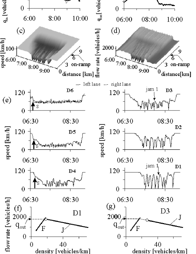
Figure 8: Simulation of GP evolution: (a, b) – Time dependences of flow rates $q_{\rm in}$ (a) and $q_{\rm on}$ (b). (c, d) – Speed (c) and flow rate (d) averaged across the road in space and time for spontaneous GP emergence and evolution. (e) – Speed at different detectors as a function of time for the GP. (f) – The line $J$ when free flow (left) and synchronized flow (right) is formed in the wide moving jam outflow for the wide moving jam labeled $``$jam 1” within the GP in (e). $q_{\rm out}$ is the flow rate in free flow formed by the wide moving jam outflow.

For numerical simulation of empirical GP occurrence and evolution at an on-ramp bottleneck (Fig. 5 (b, c)), a model of two-lane freeway with an on-ramp bottleneck is used (Sect. 16.2 in KernerBook ). At the upstream boundary of the main road, the time-dependence of the flow rate $q_{\rm in}(t)$ associated with empirical data measured at the detector D1 has been applied (Fig. 8 (a, b)). Empirical detector measurements (Fig. 5 (b, c)) are compared with simulated results at the same virtual detector locations D1–D6 as those in empirical data. As wide moving jams are observed during the time interval 7:15–9:00 at the farthest available upstream detector D1, the flow rate $q_{\rm in}(t)$ is approximated by a line. The flow rate to the on-ramp $q_{\rm on}(t)$ used in the simulations is taken from measurements in the on-ramp lane.

In simulations, GP emergence and evolution (Fig. 8 (c, d)) are qualitatively and quantitatively the same as those in empirical observations (Fig. 5). In particular, in accordance with the empirical study, the following main effects are found:

(i) A local first-order F$\rightarrow$S transition at the bottleneck (labeled $S$ at D6, Fig. 8 (e)). Over time traffic demand ($q_{\rm on}(t)$ and $q_{\rm in}(t)$) in an initial free flow at the on-ramp bottleneck increases. Whereas at D7 just downstream of the bottleneck and just upstream of the bottleneck at D5 free flow remains, at D6 within the merging region of the on-ramp an abrupt decrease in speed is observed.

(ii) A probabilistic nature of the F$\rightarrow$S transition: In different realizations performed at the same $q_{\rm on}(t)$ and $q_{\rm in}(t)$, an F$\rightarrow$S transition can occur at different flow rates at the bottleneck.

(iii) Upstream propagation of a wave of induced F$\rightarrow$S transitions. Whereas free flow further remains at D7 downstream of the bottleneck, F$\rightarrow$S transitions are induced by upstream propagation of the upstream front of synchronized flow (labeled $S$ in Fig. 8 (e), D5 and D4).

(iv) Pinch region formation with narrow moving jam emergence within synchronized flow. A self-compression of synchronized flow upstream of the bottleneck (D5, D4) is observed: Average speed decreases and density increases. In this pinch region, narrow moving jams emerge and grow in amplitude propagating upstream.

(v) Formation of wide moving jams. Some of narrow moving jams transform into wide moving jams (D3). As a result, a region of wide moving jams upstream of the pinch region is formed (D3–D1). Wide moving jams propagate upstream while maintaining the mean velocity of their downstream front. In the wide moving jam outflow either free flow or synchronized flow can occur. In the first case, in the flow–density plane the line $J$ reaches free flow region (Fig. 8 (f)). In the second case, the left co-ordinates of the line $J$ are related to the average speed and flow rate in synchronized flow (Fig. 8 (g)).

(vi) Strong congestion conditions. During the time before $t\approx$ 8:00, strong congestion conditions are realized in the pinch region. The average flow rate (10 min averaging time interval) displays only minor changes in the vicinity of the limit (minimum) flow rate $q^{\rm(pinch)}_{\rm lim}$, which does not depend on traffic demand, specifically when the flow rates $q_{\rm on}(t)$ and $q_{\rm in}(t)$) increase; the frequency of narrow moving jam emergence reaches the maximum possible value for chosen model parameters.

(vii) GP evolution. When the flow rates $q_{\rm on}(t)$ and $q_{\rm in}(t)$ begin to decrease, the initial GP under the strong congestion condition transforms into an GP under the weak congestion condition. In this case, the average speed in the pinch region increases and the average flow rate ceases to be a self-sustaining value that is close to $q^{\rm(pinch)}_{\rm lim}$; the frequency of narrow moving jam emergence in the pinch region decreases.

(viii) Return S$\rightarrow$F transitions. When the flow rates $q_{\rm on}(t)$ and $q_{\rm in}(t)$ further decrease, return S$\rightarrow$F transitions firstly occur upstream of the bottleneck and later at the bottleneck. As a result, the congested pattern dissolves and free flow returns at the bottleneck.

(ix) Hysteresis Effects. At each detector location F$\rightarrow$S and return S$\rightarrow$F transitions cause hysteresis effects in the flow–density plane Hysteresis .

III.1.2 WSP Emergence and its Transformation into GP and EP

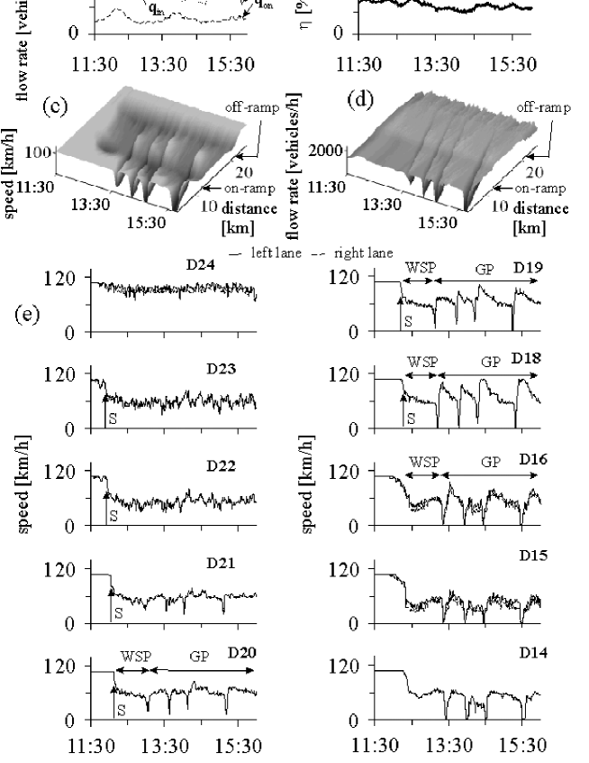
Figure 9: Simulations of congested pattern evolution at two adjacent bottlenecks: (a, b) – Time dependences of flow rates $q_{\rm in}$, $q_{\rm on}$ (a) and the percentage of vehicles $\eta$ that leave the main road to the off-ramp (b). (c, d) – Speed (c) and flow rate (d) averaged across the road in space and time. (e) – Speed at different detectors as a function of time. $v_{\rm free\ off}=$ 65 km/h.

For numerical simulation of WSP emergence at an off-ramp bottleneck and the subsequent WSP transformation into an EP and an GP at an on-ramp bottleneck (Fig. 6), the same model as in Sect. III.1.1, however, with an off-ramp bottleneck downstream and an on-ramp bottleneck upstream is used. At the road upstream boundary, the time-dependence of the flow rate $q_{\rm in}(t)$ associated with empirical data measured at the detector D8 (see Fig. 2.2 in KernerBook ) has been applied. During the time interval, when wide moving jams are observed, $q_{\rm in}(t)$ is approximated by a line (Fig. 9 (a)) as in Sect. III.1.1. The flow rate to the on-ramp $q_{\rm on}(t)$ is taken from measurements in the on-ramp lane. The empirical flow rate to the off-ramp $q_{\rm off}(t)$ is used to calculate the percentage of vehicles $\eta(t)$ in the flow rates $q_{\rm in}(t)$ and $q_{\rm on}(t)$, which leave the main road to the off-ramp (Fig. 9 (b)).

In simulations, congested pattern emergence and evolution (Fig. 9) are qualitatively the same as those in empirical observations (Fig. 6). In particular, in accordance with the empirical study (Fig. 6), the following main effects are found:

(i) A local first-order F$\rightarrow$S transition occurs at some distance upstream of the off-ramp bottleneck (D23, labeled $S$ in Fig. 9 (e)). A wave of induced F$\rightarrow$S transitions propagates upstream (labeled $S$ in Fig. 9 (e), at D22–D18). A widening synchronized flow pattern (WSP) is formed due to these F$\rightarrow$S transitions.

(ii) Transformation of the WSP into an expanded pattern (EP). After the upstream front of the WSP reaches the upstream bottleneck (on-ramp bottleneck), this front induces an F$\rightarrow$S transition at the on-ramp bottleneck (D16 in Fig. 9 (e)). Due to subsequent propagation of this synchronized flow front upstream of the on-ramp bottleneck, the EP occurs in which synchronized flow affects both downstream and upstream bottlenecks.

(iii) Intensification of downstream congestion due to upstream congestion. After the EP has appeared, wide moving jams begin to form downstream of the on-ramp bottleneck within synchronized flow of the initial WSP: The initial WSP transforms into an GP between the off-ramp and on-ramp bottlenecks. This intensification of downstream congestion (congestion formation upstream of the off-ramp bottleneck) due to upstream congestion (congestion upstream of the on-ramp bottleneck) exhibits the same features as those in empirical data (Sect. II.4.2).

(iv) Hysteresis Effect of Pattern Existence. At $t>$13:30 the flow rates $q_{\rm on}(t)$ and $q_{\rm in}(t)$ become appreciably smaller than at the time of the F$\rightarrow$S transition at the off-ramp bottleneck. Nevertheless, due to the hysteresis effect of congested pattern existence the EP persists during a very long time affecting both bottlenecks.

III.1.3 Spatial Dependence of Macroscopic Congested Traffic Pattern Characteristics

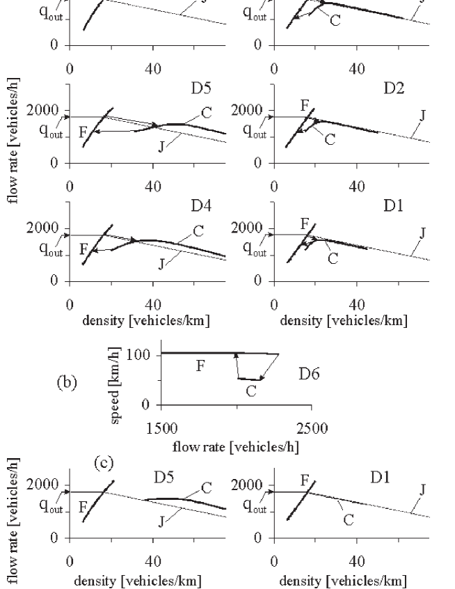
Figure 10: Fundamental diagrams and Z-characteristic: (a, b) – Theoretical spatial dependence of the fundamental diagram (a) and the Z-characteristic for the F$\rightarrow$S transition at the bottleneck (D6) (b) for the GP shown in Fig. 8. (c) – Theoretical fundamental diagrams for GP under strong congestion. Arrows in (a, b) show F$\rightarrow$S transitions (from the branch $F$ to the branch $C$) and S$\rightarrow$F transitions (from the branch $C$ to the branch $F$) at the related detectors.

Spatial theoretical dependences of the fundamental diagrams and speed correlation functions are qualitatively the same (Figs. 10 and 11) as those characteristics in empirical investigations (Fig. 7 and Fig. 12.8 in KernerBook ), respectively.

At the on-ramp bottleneck (D6), the fundamental diagram (Fig. 10 (a)) is associated with the Z-shaped speed–flow rate characteristic (Fig. 10 (b)) that is usual for a first-order F$\rightarrow$S transition KernerBook ; Z_Hom ; on the branch for synchronized flow (branch $C$) the flow rate is an increasing density function. In the pinch region of the GP (D5), the fundamental diagram exhibits a maximum point: At greater densities the flow rate slightly decreases with density, whereas at smaller densities the flow rate is a weak increasing density function. At greater densities associated with the strong congestion condition, the branch $C$ lies above the line $J$. This is related to growing character of narrow moving jams in the pinch region. If only the time interval for the strong congestion condition within the pinch region of the GP is considered, the flow rate is approximately constant: It is only a very weak density function (D5, Fig. 10 (c)). Upstream of the pinch region, the greater the distance a freeway location from the pinch region, the closer the branch $C$ to the line $J$ at greater densities. Within the completely formed region of wide moving jams (D2, D1), the branch $C$ lies on the line $J$ at greater densities. If the time interval in which only wide moving jams are observed is considered, the branch $C$ lies on the line $J$ for all densities (D1, Fig. 10 (c)) Wide_J .

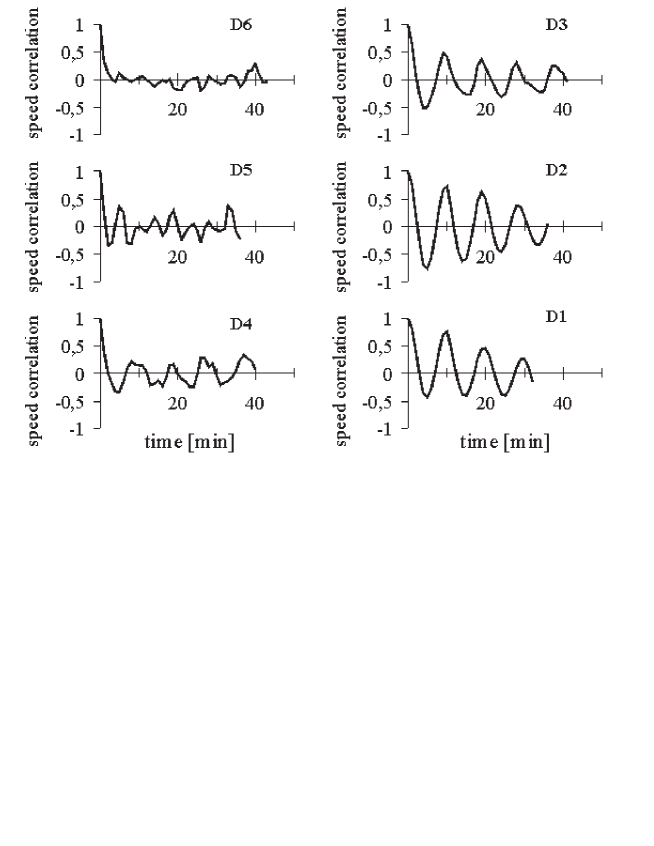
Figure 11: Simulated speed correlation functions at different detectors for the GP in Fig. 8.

The speed correlation function for the GP (Fig. 11) exhibits the same features as those in empirical results.

III.2 Simulations of Microscopic Criterion for Wide Moving Jam

Simulations show that the microscopic criterion for wide moving jam phase presented in Sect. II.2 enable us to distinguish clearly between the wide moving jam and synchronized flow phases in local microscopic (single vehicle) congested traffic states.

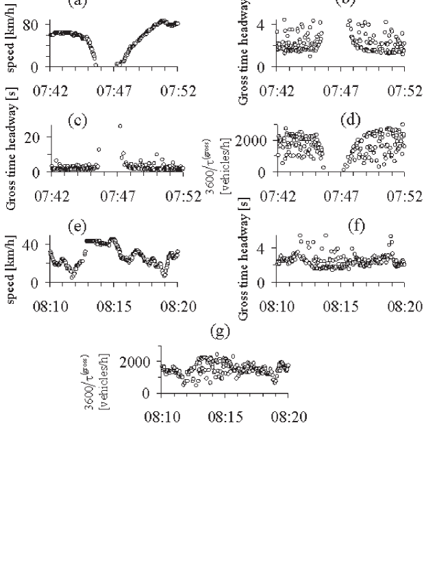
Figure 12: Simulations of microscopic criterion for traffic phase identification in different local microscopic congested traffic states related to different locations within the GP shown in Fig. 8 (c–e): (a–d) – Single vehicle model data related to the location D2 for speed within a wide moving jam in the left lane (a) and the associated time distributions of gross time headways $\tau^{\rm(gross)}$ for different scales of the headways (b, c) and of the value $3600/\tau^{\rm(gross)}$ (d). (e–g) – Single vehicle model data related to the location D4 for speed within a sequence of two narrow moving jams in the left lane (e) and the associated time distributions of $\tau^{\rm(gross)}$ (f) and of $3600/\tau^{\rm(gross)}$ (g).

Indeed, in Fig. 12 the same dependences and characteristics as those in empirical results (Fig. 2) are presented for a wide moving jam (Fig. 12 (a–d)) and two narrow moving jams (Fig. 12 (e–g)) associated with two different local microscopic congested traffic states related to two different locations within the GP in Fig. 8 (c–e). A comparison of the empirical (Fig. 2) with related simulated results (Fig. 12) fully confirms all conclusions about the traffic phase identification in congested traffic formulated in Sect. II.2. In addition, within model wide moving jams there are often gross time headways between vehicles that are about 4–7 sec. As found, they are related to moving blanks within the jams. This confirms the assumption made in Sect. II.2 that such gross time headways within empirical wide moving jams are explained by moving blanks.

If the microscopic criterion is applied for the moving jams, which propagate through the on-ramp bottleneck in Fig. 9 (e), then we find that within each of these jams traffic interruption occurs, i.e., the condition (1) is satisfied. This means that corresponding to the microscopic criterion these moving jams are wide moving jams. The same conclusion is made from the macroscopic spatiotemporal objective criteria for traffic phases in congested traffic. Indeed, these jams propagate through the bottleneck while maintaining the mean jam downstream front velocity. Thus, the microscopic criterion and macroscopic objective spatiotemporal criteria for the traffic phases lead to the same result by phase identification in congested traffic.

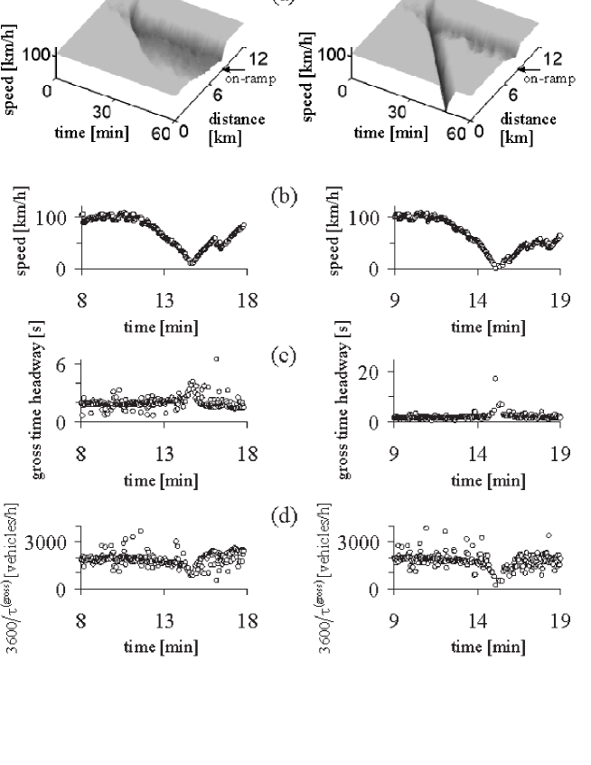
Figure 13: Comparison of microscopic criterion with macroscopic spatiotemporal objective criteria for the phases in congested traffic. Figures left are related to a narrow moving jam, figures right are related to a wide moving jam: (a) – The catch effect of a narrow moving jam at an on-ramp bottleneck with subsequent LSP formation at the bottleneck (left) and wide moving jam propagation through the bottleneck with LSP formation at the bottleneck (right). Average vehicle speed (one-minute data) in space and time. (b) – Single vehicle model data for vehicle speed. (c, d) – gross time headways (c) and the value $3600/\tau^{\rm(gross})$ (d) related to (b). $q_{\rm in}=$ 1830, $q_{\rm on}=$ 270, $q_{\rm out}=$ 1810 vehicles/h/lane.

To prove the latter conclusion, a numerical experiment is performed additionly (Fig. 13). In this numerical experiment, metastable free flow is realized at an on-ramp bottleneck. Firstly, a narrow moving jam is induced downstream of the on-ramp bottleneck (Fig. 13 (a), left). Indeed, an application of the microscopic criterion to this moving jam shows (Fig. 13 (b–d), left) that there is no traffic interruption within the jam. In this case, we find $\tau^{\rm(gross)}_{\rm max}/\tau^{\rm(ac)}_{\rm del}\approx$ 2 (model time delay $\tau^{\rm(ac)}_{\rm del}\approx$ 1.74 sec). Rather than the jam propagating through the on-ramp bottleneck, the moving jam is pinned at the bottleneck leading to an F$\rightarrow$S transition with subsequent localized SP (LSP) formation upstream of the bottleneck (Fig. 13 (a), left). Secondly, another moving jam is induced at the same location downstream of the bottleneck (Fig. 13 (a), right). However, there is flow interruption within this jam (Fig. 13 (b–d), right). Accordingly to the microscopic criterion for the phases in congested traffic, this jam is a wide moving jam. In this case, we find $\tau^{\rm(gross)}_{\rm max}/\tau^{\rm(ac)}_{\rm del}\approx$ 10. In contrast with former narrow moving jam, this jam propagates through the bottleneck while maintaning the mean downstream jam front velocity (Fig. 13 (a), right). As in empirical observations KernerBook , wide moving jam propagation through metastable free flow state at the bottleneck leads to LSP formation as in the case of the former narrow moving jam. In contrast with the narrow moving jam, synchronized flow within the LSP has no influence on wide moving jam propagation (Fig. 13 (a), right). It is found that to identify a moving jam as a wide moving jam based on the microscopic criterion with certainty the following numerical relation should be satisfied $\tau^{\rm(gross)}_{\rm max}/\tau^{\rm(ac)}_{\rm del}>$ 5.

The relative large number 5 found for this criterion is associated with fluctuations. We have found that in some of different realizations made at the same flow rates and initial conditions for jam excitation, when 3 $<\tau^{\rm(gross)}_{\rm max}/\tau^{\rm(ac)}_{\rm del}<$ 5, a moving jam is a wide moving jam (it propagates through the bottleneck while maintaining the mean velocity of the jam downstream front), but in the other realizations the jam is a narrow moving jam (it is pinned at the bottleneck causing an F$\rightarrow$S transition at the bottleneck). This is because of fluctuations of vehicle motion within the jam, in the jam inflow and outflow, as well as fluctuations through random vehicle lane changing. In particular, it can turn out that within a moving jam a vehicle changes lane before it passes the detector. Then a time headway measured by the detector increases. This random lane changing has obviously no relation to flow interruption within a moving jam. A more detailed study of fluctuations is beyond the scope of this article.

III.3 Spatial Dependence of Single Vehicle Model Characteristics

Here, single vehicle model characteristics associated with the GP at the on-ramp bottleneck are compared with empirical results. However, the GP in Fig. 8 exists about two hours only. In order to make more reliable statistical characteristics from single vehicle model data, after the flow rates $q_{\rm on}(t)$ and $q_{\rm in}(t)$ taken from measurements reach their maximum values, these flow rates do not change in simulations any more. Then an GP that occurs at the bottleneck does not dissolve over time at all. The characteristics of this GP are the same as those for the GP in Fig. 8 (c–e) before 8:00.

III.3.1 Model Time Headway Distributions and OV Functions

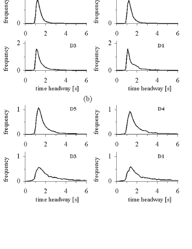
Figure 14: Model time headway distributions at different detectors within general patterns: (a) – Simulations of the model of identical vehicles related to Fig. 8 (e). (b) – Simulations of the model for heterogeneous flow with various driver and vehicle characteristics of Sect. 20.2 in KernerBook with 30$\%$ of fast, 35$\%$ of slow, and 35$\%$ of long vehicles; $v^{(1)}_{\rm free}=$ 120 km/h; other parameters for fast vehicles are the same as those for identical vehicles in Sect. 16.3 of Ref. KernerBook ; $\tau^{\rm(a,\ j)}_{\rm del}(v)=\tau/p^{(j)}_{0}(v)$, $p^{(j)}_{0}(v)=(a^{(j)}+b^{(j)}\min(1,\ v/10))$, $j=2,3$; $a^{(2)}=0.42,\ b^{(2)}=0.13$ for slow vehicles ($j=$ 2) and $a^{(2)}=0.3,\ b^{(2)}=0.18$ for long vehicles ($j=3$).

Time headway distributions related to synchronized flow (D5, D4, Fig. 14 (a)) are qualitatively the same as empirical ones (Fig. 3). In the model, time intervals between wide moving jams at D3–D1 (Fig. 8 (e)) are considerably shorter than in the empirical example 1 (Fig. 1 (b)). For this reason, longer time headways associated with moving blanks within wide moving jams can be seen in the model time headway distributions (D1, Fig. 14 (a)) even without speed separation of time headways made in Fig. 3 (b).

Quantitative differences between empirical and model results (Figs. 3 and 14 (a)) at small time headways are explained by model time step that is equal to 1 sec, i.e., considerably shorter time headways cannot be observed.

There are very different vehicles and drivers in real traffic, specifically aggressive and timid driver behavior are related to shorter and longer drivers’ time delays, respectively. In the model of identical vehicles and drivers used above, chosen driver time delays are more close to aggressive drivers rather than to timid ones. This explains why longer time headways do not appear in the model time headway distributions in Fig. 14 (a). If the microscopic model with various drivers (Sect. 20.2 in KernerBook ) is used, then a quantitative correspondence with any known empirical result of time headway distributions through the appropriate choice of the percentage of slow (timid) drivers and their characteristics is possible (Fig. 14 (b)). It is important that in this case the fundamental spatiotemporal features of congested patterns discussed above do not change, as this has been found in KKl2004AA .

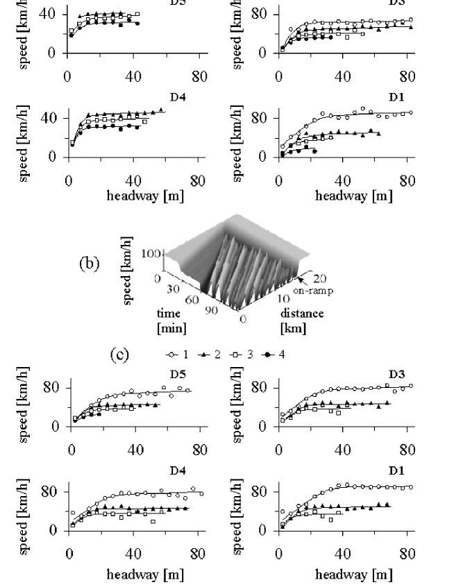
Figure 15: Model OV functions at different detectors within general patterns: (a) – Simulations of the model of identical vehicles related to Fig. 8 (e). (b, c) – Simulations of an GP (b) and associated OV functions (c) for the KKW CA model (Sect. 20.2 in KernerBook ). Curves 1–4: $\rho=$ 20–30, $\rho=$ 30–40, $\rho=$ 40–50, and $\rho=$ 50–60 vehicles/km, respectively.

Model OV functions (Fig. 15 (a)) show the same characteristics as those for the empirical OV functions (Fig. 4). This is true for the models with identical vehicles and with various drivers’ and vehicles’ characteristics. The same conclusion can be drawn for the KKW CA model (Fig. 15 (b, c)), in which under the same conditions as those in Fig. 8 an GP, which is qualitatively the same, occurs at the on-ramp bottleneck (Fig. 15 (b)) KKW_model .

III.3.2 Speed Adaptation Functions

Analyzing single vehicle data, in Ref. Wagner_Lub_2003A it has been found that in congested traffic a distribution $p_{\delta v}(\delta v)$ for vehicle speed difference $\delta v=v_{i+1}-v_{i}$ associated with two vehicles $i$ and $i+1$, which are registered at a detector location one after another, have a very sharp maximum at $\delta v=0$: There is an attraction of vehicles to a region with a very small speed difference in congested traffic.

This behavior has been explained by the speed adaptation effect KKl2004AA ; KernerBook : If a vehicle cannot overtake the preceding vehicle, then within a synchronization distance the vehicle tends to adapt the vehicle speed to the speed of the preceding vehicle, i.e., the speed difference $\delta v\rightarrow 0$. The less the probability of overtaken, the more vehicles due to the speed adaptation effect should move with small speed difference $\delta v$ to each other. The probability of overtaken is a decreasing function of the speed. The decrease of probability of overtaken becomes appreciable already at higher densities in free flow. When synchronized flow occurs, probability of overtaken drops abruptly. Specifically, there is a strong attraction of vehicles in synchronized flow to a region with small speed difference associated with the speed adaptation effect within the synchronization distance. As a result, the function $p_{\delta v}(\delta v)$ has a very sharp maximum in synchronized flow.

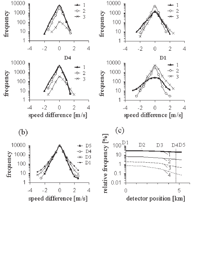
Figure 16: Simulations of speed adaptation effect at different detector locations within the GP in Fig. 8 (e): (a) – Frequency $p_{\delta v}$ as a function of $\delta v$ for different ranges of the space headway : curves 1 – 0–12.5 m, curves 2 – 12.5–25 m, curves 3 – $>$ 25 m (densities $\rho>$ 50 vehicles/km, $30<\rho<50$, and $\rho<$ 30 vehicles/km, respectively). (b) – Frequency $p_{\delta v}$ as a function of $\delta v$ at different detectors regardless of space headways. (c) – Spatial dependence of relative frequency $p_{\delta v}/p_{0}$ at different given values of the speed difference $\delta v$: curve 1 – $\delta v=\pm$ 0.5 m/s, curve 2 – $\delta v=\pm$ 1 m/s, curve 3 – $\delta v=\pm$ 1.5 m/s, curve 4 – $\delta v=\pm$ 2.0 m/s. $p_{0}=p_{\delta v}\mid_{\delta v=0}$.

This effect is found in numerical simulations at locations D6 and D5 at which synchronized flow without wide moving jams occurs (Fig. 16 (a)). However, when wide moving jams appear (D3–D1), then at a given vehicle space headway range the width of frequency distribution $p_{\delta v}(\delta v)$ increases. This means that the frequency distribution $p_{\delta v}(\delta v)$ in congested traffic is a function of the spatial co-ordinate and of local dynamics within a congested pattern (Fig. 16 (b, c)): At freeway locations within the pattern in which many wide moving jams propagate (D1, D2, Fig. 8 (e)), the distribution $p_{\delta v}(\delta v)$ at a given $\delta v$ becomes greater than at the locations at which synchronized flow without wide moving jams is realized (D5).

IV Discussion

Based on empirical and model results presented, the following conclusions can be made:

(i) A microscopic criterion for the wide moving jam phase in single vehicle data presented in the article enables us to identify qualitatively different local microscopic congested traffic states in both empirical and single vehicle model data measured at a single freeway location.

(ii) A comparison of empirical and simulated freeway traffic phenomena shows that a microscopic three-phase traffic theory of Ref. KKl ; KKW ; KKl2003A ; KKl2004AA can explain both microscopic and macroscopic empirical congested pattern features.

(iii) Empirical microscopic (single vehicle) time headway distributions and OV functions found in the article for qualitatively different empirical local microscopic congested traffic states can been reproduced in the microscopic theory for the associated different congested states satisfactorily.

(iv) Time headway distributions, and distributions for vehicle speed difference can depend on the spatial co-ordinate considerably. However, the significance of these spatial changes of the traffic characteristics depends on the congested pattern type. In particular, if wide moving jam duration is small in comparison with synchronized flow duration, then time headway distributions and frequency distributions for vehicle speed difference do not depend on the freeway location appreciably.

(v) If time-dependencies of traffic demand and drivers’ destinations related to macroscopic empirical data are given at the upstream model boundaries of the main road and an on-ramp, then simulated spatiotemporal congested patterns emerge, develop, and dissolve due to self-organization effects in traffic flow in accordance with empirical observations.

In general, main features of empirical OV functions and time headway distributions are not necessarily qualitatively different, even if local traffic dynamic characteristics within congested patterns are qualitatively different. Therefore, these and many other empirical traffic flow characteristics (e.g., global and aggregated fundamental diagrams, hysteresis effects, etc.) could be considered secondary ones in comparison to spatiotemporal traffic pattern features (item (1)–(4) in Sect. I).

This is because important spatiotemporal features of phase transitions and congested patterns (item (1)–(4) in Sect. I) are lost in these and many other macroscopic and microscopic traffic characteristics, which are widely used as the empirical basis for tests of traffic flow models. Thus, it is not justified to use these macroscopic and microscopic characteristics as the solely empirical basis for a decision whether a traffic flow model can describe real traffic flow or not NS_TEst .

Firstly, a comparison of empirical features of phase transitions in traffic flow and spatiotemporal congested patterns with associated model solutions for a model of freeway with those freeway bottlenecks, which affect the empirical patterns, has to be performed. Then microscopic model characteristics of single vehicle model data associated with different locations within the patterns are studied. Finally, these microscopic model characteristics are compared with empirical microscopic characteristics of single vehicle data. This data should be related to qualitatively the same empirical local congested model states as those in the model states.

References

- (1) B.S. Kerner. The Physics of Traffic (Springer, Berlin, New York 2004).
- (2) N.H. Gartner, C.J. Messer, A. Rathi (eds.). Special Report 165: Revised Monograph on Traffic Flow Theory (Transportation Research Board, Washington, D.C. 1997).
- (3) D.E. Wolf. Physica A 263, 438 (1999).
- (4) D. Chowdhury, L. Santen, A. Schadschneider. Physics Reports 329, 199 (2000).
- (5) D. Helbing. Rev. Mod. Phys. 73, 1067–1141 (2001).
- (6) T. Nagatani. Rep. Prog. Phys. 65, 1331–1386 (2002).
- (7) K. Nagel, P. Wagner, R. Woesler. Operation Res. 51, 681–716 (2003).
- (8) R. Mahnke, J. Kaupužs, I. Lubashevsky, Phys. Rep. 408, 1-130 (2005).
- (9) J.-B. Lesort (editor). Transportation and Traffic Theory, Proceedings of the 13th International Symposium on Transportation and Traffic Theory (Elsevier Science Ltd, Oxford 1996)
- (10) A. Ceder (editor). Transportation and Traffic Theory, Proceedings of the 14th International Symposium on Transportation and Traffic Theory (Elsevier Science Ltd, Oxford 1999)
- (11) M.A.P. Taylor (editor). Transportation and Traffic Theory in the 21st Century, Proceedings of the 15th International Symposium on Transportation and Traffic Theory (Elsevier Science Ltd, Amsterdam 2002)
- (12) D.E. Wolf, M. Schreckenberg, A. Bachem (editors). Traffic and Granular Flow, Proceedings of the International Workshop on Traffic and Granular Flow, October 1995 (World Scientific, Singapore 1995)
- (13) M. Schreckenberg, D.E. Wolf (editors). Traffic and Granular Flow’ 97, Proceedings of the International Workshop on Traffic and Granular Flow, October 1997 (Springer, Singapore 1998)
- (14) D. Helbing, H.J. Herrmann, M. Schreckenberg, D.E. Wolf (editors). Traffic and Granular Flow’ 99, Proceedings of the International Workshop on Traffic and Granular Flow, October 1999, (Springer, Heidelberg 2000)
- (15) M. Fukui, Y. Sugiyama, M. Schreckenberg, D.E. Wolf (editors). Traffic and Granular Flow’ 01, Proceedings of the International Workshop on Traffic and Granular Flow, October 2001, (Springer, Heidelberg 2003)
- (16) S.P. Hoogendoorn, P.H.L. Bovy, M. Schreckenberg, D.E. Wolf (editors). Traffic and Granular Flow’ 03, Proceedings of the International Workshop on Traffic and Granular Flow, October 2003, (Springer, Heidelberg 2005) (in press).
- (17) B. S. Kerner. Phys. Rev. Lett. 81, 3797 (1998).
- (18) B. S. Kerner, Phys. Rev. E 65, 046138 (2002).
- (19) B.S. Kerner, S.L. Klenov: J. Phys. A: Math. Gen. 35, L31 (2002)
- (20) B.S. Kerner, S.L. Klenov, D.E. Wolf, J. Phys. A: Math. Gen. 35 9971–10013 (2002).
- (21) B.S. Kerner, S.L. Klenov, Phys. Rev. 68 036130 (2003)
- (22) B.S. Kerner, S.L. Klenov, J. Phys. A: Math. Gen. 37 8753–8788 (2004).
- (23) L.C. Davis, Phys. Rev. E 69 016108 (2004).
- (24) H.K. Lee, R. Barlović, M. Schreckenberg, D. Kim, Phys. Rev. Let. 92, 238702 (2004).
- (25) R. Jiang, Q.S. Wu, J. Phys. A: Math. Gen. 37, 8197–8213 (2004).
- (26) L. Neubert, L. Santen, A. Schadschneider, M. Schreckenberg. Phys. Rev. E 60, 6480 (1999).
- (27) W. Knospe, L. Santen, A. Schadschneider, M. Schreckenberg. Phys. Rev. E 65, 056133 (2002).
- (28) W. Knospe, L. Santen, A. Schadschneider, M. Schreckenberg. Phys. Rev. E 70, 016115 (2004).
- (29) R. J. Cowan. Trans. Rec. 9, 371–375 (1976).
- (30) M. Koshi, M. Iwasaki, I. Ohkura. Some Findings and an Overview on Vehicular Flow Characteristics’. In: Procs. 8th International Symposium on Transportation and Traffic Theory ed. V. F. Hurdle, et al (University of Toronto Press, Toronto, Ontario 1983) pp. 403.
- (31) T. Luttinen. Transportation Res. Rec. 1365 (1992).
- (32) P.H.L. Bovy (editor). Motorway Analysis: New Methodologies and Recent Empirical Findings (Delft University Press, Delft 1998).
- (33) B. Tilch, D. Helbing, in: SW3 , p.333.
- (34) J. Banks. Trans. Rec. B 37, 539–554 (2004).
- (35) G.S. Gurusinghe, T. Nakatsuji, Y. Azuta, P. Ranjitkar, Y. Tanaboriboon. Multiple Car-Following Data Using Real-Time Kinematic Global Positioning System’. In: Preprints of the 82nd TRB Annual Meeting TRB Paper No.: 03-4137 (TRB, Washington D.C. 2003).
- (36) Sometimes for better statistical conclusions, traffic variables obtained from various days or/and many different locations are aggregated to a data set; this data base of aggregated data is further used for calculation of traffic flow characteristics.
- (37) Below the condition (1) is applied for vehicles in the left (passing) freeway line in which person vehicles move mostly. When there are many long vehicles in traffic flow, rather than the maximum gross time headway, the maximum time headway should be used in the condition (1) for flow interruption within a moving jam, i.e., this condition should be replaced by . This is because at a low speed of a very long vehicle within a moving jam, the condition (1) can sometimes be satisfied, if the jam is still a narrow one.
- (38) Corresponding to empirical results sec KernerBook .
- (39) A model fundamental diagram, which consists of a branch for free flow and a branch for congested traffic that entirely coincides with the line , has first been found in the Kerner-Konhäuser theory of wide moving jam propagation KK1994 (see Fig. 12 (a) in KK1994 ). The branch for congested traffic in this global fundamental diagram is related to a sequence of free flow and wide moving jam(s) on a homogeneous circular road: When the whole number of vehicles on the road increases (density averaged over the whole road increases), then the total jam width(s) on the road increases and the total width of free flow regions between the jam(s) decreases. As a result, the average flow rate decreases in accordance with the line . A free flow state, at which the braches for free flow and congested traffic merge on the fundamental diagram, corresponds to the wide moving jam outflow. The flow rate in this wide moving jam outflow is smaller than the maximum flow rate in free flow at which moving jams emerge spontaneously in free flow. Thus, this fundamental diagram has a reversed--form. Later, the same results have been found in many other traffic flow models (see references in the review Helbing2001 ). In contrast with these model results, in real traffic, when the branch for congested traffic coincides with the line (D1, Fig. 7 (b)), then this branch is related to synchronized flow states associated with the outflows from different wide moving jams. This is because in empirical investigations a variety of different synchronized flow states, all of them belong to the line , are formed in the jam outflows. This is in accordance with results of three-phase traffic theory KernerBook . In contrast, two-phase traffic theories KK1994 ; Helbing2001 can explain only two points on the empirical branch for congested traffic: The point associated with the flow rate in the jam outflow at which the braches for free flow and congested traffic merge on the fundamental diagram and the point within the jam KernerBook .
- (40) B.S. Kerner, P. Konhäuser. Phys. Rev. E 50, 54–83 (1994).
- (41) From a comparison of a local traffic dynamics measured at D2 (not shown) with the dynamics at D1 in Fig. 1 (b) (example 1) has been found that the moving jams propagate upstream with the mean velocity of the downstream jam fronts 15.8 km/h.
- (42) It must be noted that during these FSF hysteresis effects traffic flow is not interrupted. This is qualitatively different from FJF, SJS, SJF, and FJS hysteresis effects” in the flow–density plane caused by wide moving jam propagation through a detector location. In the latter cases, there is flow interruption within the jam (Sect. II.2): The jam inflow is independent of the jam outflow (, if free flow is formed in the jam outflow). When , i.e., the jam width increases over time, the flow rate measured at the detector becomes smaller after wide moving jam propagation through the detector location. In contrast, when , i.e., the jam width decreases over time, the flow rate becomes greater after wide moving jam propagation. Thus, a very complex hysteresis effects” in the flow–density plane are possible. For their understanding, a spatiotemporal analysis of traffic pattern emergence and evolution is necessary.
- (43) Our investigations show that the theoretical fundamental diagram, which follows from a Z-dependence for an FS transition on a homogeneous road KKl2003A (see Fig. 17.3 (a) in KernerBook ), is also qualitatively the same as those for empirical synchronized flow within a moving SP that emerges away from bottlenecks KernerBook (see Fig. 10.13 (a) in KernerBook ).
- (44) As follows from Fig. 15 (b, c), OV functions presented in Ref. Knospe2004 with the reference to the KKW CA model are not associated with the KKW CA model. Thus, conclusions about microscopic features of the KKW CA model made in Ref. Knospe2004 are incorrect.
- (45) P. Wagner, I. Lubashevsky. cond-mat/0311192 (2003).
- (46) In particular, the analysis made explains why the Nagel-Schreckenberg CA model and its variants NS , which in accordance with KKW cannot show and predict the main empirical spatiotemporal features of traffic flow (item (1)–(4) in Sect. I), even though the models show the global empirical fundamental diagram, empirical OV functions and time headway distributions satisfactory, as found in the empirical test of these models Knospe2004 .
- (47) K. Nagel, M. Schreckenberg: J Phys. (France) I 2, 2221 (1992); K. Nagel, M. Paczuski. Phys. Rev. E 51, 2909 (1995); M. Schreckenberg, A. Schadschneider, K. Nagel, N. Ito. Phys. Rev. E 51, 2939 (1995); R. Barlović, L. Santen, A. Schadschneider, M. Schreckenberg. Eur. Phys. J. B. 5, 793 (1998); W. Knospe, L. Santen, A. Schadschneider, M. Schreckenberg. J. Phys. A 33, L477 (2000).