On the origin of the gravitational quantization: The Titius–Bode Law

Abstract.

Action at distance in Newtonian physics is replaced by finite propagation speeds in classical post–Newtonian physics. As a result, the differential equations of motion in Newtonian physics are replaced by functional differential equations, where the delay associated with the finite propagation speed is taken into account. Newtonian equations of motion, with post–Newtonian corrections, are often used to approximate the functional differential equations. In [8] a simple atomic model based on a functional differential equation which reproduces the quantized Bohr atomic model was presented. The unique assumption was that the electrodynamic interaction has finite propagation speed. Are the finite propagation speeds also the origin of the gravitational quantization? In this work a simple gravitational model based on a functional differential equation gives an explanation of the modified Titius–Bode law.

1. Introduction

In the last two centuries several attempts were made to express and explain the distribution of the planetary orbits and other relevant quantities using integer numbers. Titius (1772) and Bode (1776) (see for instance [12, 22]) proposed the law describing the mean distances of planets from the Sun of the general form

$$r_{n}=a+b\,c^{n},$$

where $r_{n}$ means distance characterized by an integer number $n$. The constants $a$, $b$ and $c$ have no convincing physical meaning, neither have the empirical correlations with definite parameters for a given system. Therefore, this law has raised many discussions. Nevertheless, it played a positive role not only in predicting unknown planets, but also in stimulating many researches to further work in this direction. In [11] and [20] there are some reviews about the attempts to test and to explain the Titius-Bode law.

As a precursor of the modified Titius-Bode law, Gulak [9] proposed that the orbital distances are given by $r_{n}=(n+1/2)r_{0}$ or $r_{n}=nr_{0}$, where $r_{0}$ is a characteristic of a given system. Here $n$ needs not to increase by 1 in going from one planet or satellite to another one. Gulak [10] found a theoretical support to his previous results by constructing an equation of the Schrödinger type. In this way, he tried to introduce the macroquantization of orbits in a gravitational field.

In the last years the idea that of a quantization of the gravitational field has been constated. In words of Halton Arp (see [2]): An unexpected property of astronomical objects (and therefore an ignored and suppressed subject) is that their properties are quantized, for instance the redshifts of galaxies. The most astonishing result was then pointed to by Jess Artem, that the same quantization ratio that appeared in quasar redshifts appeared in the orbital parameters of the planets in the solar system. Shortly, afterward Oliveira Neto et al. [16], Agnese and Festa [1], L. Nottale et al. [14, 15] and A. and J. Rubčić [20, 21] independently in Brazil, Italy, France and Croatia began pointing out similarities to the Bohr atom in the orbital placement of the planets. Different variations of the Bohr-like $r_{n}=n^{2}$ or $r_{n}=n^{2}+n/2$ fit the planetary semimajor axes extremely well with rather low ”quantum” numbers $n$. It is clear that the properties of the planets are not random and that they are in some way connected to quantum mechanical parameters both of which are connected to cosmological properties.

Action at distance in Newtonian physics is replaced by finite propagation speeds in classical post–Newtonian physics. As a result, the differential equations of motion in Newtonian physics are replaced by functional differential equations, where the delay associated with the finite propagation speed is taken into account. Newtonian equations of motion, with post–Newtonian corrections, are often used to approximate the functional differential equations, see, for instance, [3, 4, 5, 6, 7, 18, 19]. In [8] a simple atomic model based on a functional differential equation which reproduces the quantized Bohr atomic model was presented. The unique assumption was that the electrodynamic interaction has finite propagation speed, which is a consequence of the Relativity theory. An straightforward consequence of the theory developed in [8], and taking into account that gravitational interaction has also a finite propagation speed, is that the same model is applicable to the gravitational 2-body problem. In the following section we present a simple gravitational model based on a functional differential equation which gives an explanation of the modified Titius–Bode law.

2. The retarded gravitational 2-body problem

We consider two particles of masses $m$ and $M$, with $m\ll M$, interacting through the retarded inverse square force. The force on the mass $m$ exerted by the mass $M$ is given by

(1) $${\bf F}=G\frac{M\,m}{r^{3}}\ {\bf r}.$$

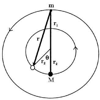
Figure 1. The retarded gravitational 2-body problem.

The force acts in the direction of the 3–vector ${\bf r}$, along which the mass $M$ is ”last seen” by the mass $m$. The 3–vector ${\bf r}$ may be represented by

$${\bf r}={\bf r}_{M}(t-\tau)-{\bf r}_{m}(t),$$

where ${\bf r}_{M}(t)$ and ${\bf r}_{m}(t)$ denote respectively the instantaneous position vectors of the mass $M$ and the mass $m$, respectively, at time $t$, and $\tau$ is the delay, so that ${\bf r}_{M}(t-\tau)$ is the ”last seen” position of the mass $M$. Assuming that the two bodies are in rigid rotation with constant angular velocity $\omega$, and referring back to Fig. 1, we have, in 3–vector notation,

$${\bf r}_{m}=r_{1}[\cos\omega t\ {\bf\hat{\i}}+\sin\omega t\ {\bf\hat{\j}}],$$

and

$${\bf r}_{M}=-r_{2}[\cos\omega(t-\tau)\ {\bf\hat{\i}}+\sin\omega(t-\tau)\ {\bf\hat{\j}}].$$

Hence, the 3–vector ${\bf r}$ is given by

$${\bf r}=[-r_{2}\cos\omega(t-\tau)-r_{1}\cos\omega t]\ {\bf\hat{\i}}+[-r_{2}\sin\omega(t-\tau)-r_{1}\sin\omega t]\ {\bf\hat{\j}},$$

Now, we introduce the polar coordinates $(r,\theta)$ and define the unitary vectors ${\bf l}=\cos\theta\ \hat{\i}+\sin\theta\ \hat{\j}$ and ${\bf n}=-\sin\theta\ \hat{\i}+\cos\theta\ \hat{\j}$. By straightforward calculations it is easy to see that the components of the force (1) in the polar coordinates are

$$F_{r}=G\frac{M\,m}{r^{3}}{\bf r}\cdot{\bf l}=(-r_{2}\cos(\omega\tau)-r_{1})G\frac{M\,m}{r^{3}}\,$$

and

$$F_{\theta}=G\frac{M\,m}{r^{3}}{\bf r}\cdot{\bf n}=r_{2}\sin(\omega\tau)G\frac{M\,m}{r^{3}}\,$$

The equations of the movement are

(2) $$m\ddot{r}-mr\dot{\theta}^{2}=F_{r},$$

(3) $$mr\ddot{\theta}+2m\dot{r}\dot{\theta}=F_{\theta}.$$

The second equation (3) can be written in the form

(4) $$\frac{1}{r}\frac{dL}{dt}=\frac{1}{r}\frac{d}{dt}(mr^{2}\dot{\theta})=F_{\theta}=r_{2}\sin(\omega\tau)G\frac{M\,m}{r^{3}}.$$

If we accurately study equation (4) we see that the analytic function $\sin(\omega\tau)$ has a numerable number of zeros given by

(5) $$\omega\tau=k\pi\,,$$

with $k\in\mathbb{Z}$, which are stationary orbits of the system of equations (2) and (3). When $\omega\tau\neq k\pi$ we have a torque which conduces the mass $m$ to the stationary orbits without torque, that is, with $\omega\tau=k\pi$. In fact the stationary orbits are limit cycles in the sense of the qualitative theory developed by Poincaré, see [17].

This is a new form of treating the gravitational 2-body problem from a dynamic point of view instead of from a static point of view, as it has been made up to now. Moreover, in this model the delay $\tau$ is not small, in fact

$$\tau=\frac{k\pi}{\omega}=\frac{k\pi}{2\pi/T}=\frac{kT}{2}\,,$$

where $T$ is the time taken by the mass $m$ to complete its orbit, i.e., the period of revolution. Therefore, the delay is a multiple of the half–period $T/2$.

On the other hand, in a first approximation, the delay $\tau$ can be equal to $r/c$ (the time that the field uses to goes from the mass $M$ to the mass $m$ at the speed of the light). In this case, from equation (5) we have

(6) $$\tau=\frac{k\pi}{\omega}=\frac{r}{c}\,.$$

Taking into account that $\omega=v_{\theta}/r$, from (6) we have $v_{\theta}/c=k\pi$. However, from the Relativity theory we know that $v_{\theta}/c<1$, then we must introduce a new constant $g$ in the delay. Hence, $\tau=g\,r/c$ and the new equation (6) is

(7) $$\tau=\frac{k\pi}{\omega}=\frac{g\,r}{c}\,,$$

and now $v_{\theta}/c=k\pi/g$, i.e. $v_{\theta}=k\pi c/g$ and from (7) we also have $r=k\pi c/(g\omega)$. In our model case of a classical rigid rotation we have $\theta=\omega t$ with $\omega>0$. Therefore, $\dot{\theta}=\omega$ and $\ddot{\theta}=0$. Hence, equation (3) for $\omega\tau=k\pi$ is

$$2m\dot{r}\omega=0,$$

which implies $\dot{r}=0$ and $r=r_{k}$ where $r_{k}$ is a constant for each $k$. On the other hand, equation (2) for $\omega\tau=k\pi$ takes the form:

(8) $$-mr\dot{\theta}^{2}=-m\frac{v_{\theta}^{2}}{r}=(-r_{2}(-1)^{n}-r_{1})G\frac{M\,m}{r^{3}}\approx-r\ G\frac{M\,m}{r^{3}},$$

assuming that $r\sim r_{1}$ due to $r_{2}\ll r_{1}$ in the case that $m\ll M$.

From the definition of angular momentum $L=mr^{2}\dot{\theta}=mr^{2}\omega=mrv_{\theta}$ we have that $v_{\theta}=L/(mr)$. Substituting this value of $v_{\theta}$ into equation (8) we obtain $r=L^{2}/(GM\,m^{2})$. The energy of the mass $m$ (substituting the values of $v_{\theta}$ and $r$) is given by

(9) $$E=\frac{mv_{\theta}^{2}}{2}-G\frac{M\,m}{r}=-\frac{G^{2}M^{2}\,m^{3}}{2\,L^{2}}.$$

The angular momentum for $\omega\tau=k\pi$ is

(10) $$L=mv_{\theta}r=m\frac{k\pi c}{g}\frac{L^{2}}{GM\,m^{2}},$$

which is an equation for the angular momentum. Isolating the value of $L$ we obtain $L=(GM\,m\,g)/(k\pi c)$. If we introduce this value of the angular momentum in the expression of the energy (9) we have

(11) $$E=-\frac{m\pi^{2}c^{2}}{2g^{2}}k^{2}.$$

The adimensional constant $g$ cannot be unambiguously determined, and it must be computed according with the experimental data. However, one may speculate by considering the similarity between the gravitational constant force $F_{g}$ and the electrodynamic force $F_{e}$. The absolute ratio of the forces is

$$\frac{F_{g}}{F_{e}}=\frac{GM\,m}{e^{2}/4\pi\varepsilon_{0}},$$

where $\varepsilon_{0}$ is the electric permittivity constant of vacuum. By introducing the well-known fine structure constant $\alpha$ defined by

$$\alpha=\frac{e^{2}}{4\pi\varepsilon_{0}\hbar c},$$

the ratio may be expressed by

$$\frac{F_{g}}{F_{e}}=\frac{1}{\alpha}\left(\frac{GM\,m}{\hbar c}\right)=\frac{\alpha_{g}}{\alpha},$$

where $\alpha_{g}$ is the adimensional gravitational fine structure constant, see [13]. However, this value of the adimensional gravitational fine structure constant does not agree with the experimental data given in the works [1, 14, 15, 16, 20, 21]. If we recall the expression of the energy levels for the electrostatic interaction given by Bohr in 1913

$$E=-\frac{1}{2}\,m\,(\alpha c)^{2}\frac{1}{n^{2}},$$

a straightforward generalization gives us that the expression of the energy levels for the gravitational interaction

(12) $$E=-\frac{1}{2}\,m\,(\alpha_{g}c)^{2}\frac{1}{n^{2}}.$$

Therefore, comparing with (11) (identifying $n=|k|$) we must impose that the constant $g=k^{2}g_{1}$ where $g_{1}=\pi/\alpha_{g}$ and then the energy takes the form (12). Therefore we have found the value of the adimensional constant $g_{1}$ and consequently the expression of the delay $\tau$ which is

(13) $$\tau=\frac{g\,r}{c}=k^{2}\,\frac{g_{1}r}{c}=k^{2}\,\frac{\pi r}{\alpha_{g}c}.$$

In fact, we generalize the expression of the delay for the electrodynamic interaction given in [8]. From the found value of the angular momentum and the value of $v_{\theta}=\alpha_{g}c/k$ we have

(14) $$L=\frac{G\,M\,m\,g}{k\pi c}=\frac{G\,M\,m\,k}{\alpha_{g}\,c}=mv_{\theta}r=m\frac{\alpha_{g}\,c}{k}r.$$

Isolating the value of $r$ from equation (14) and identifying $n=|k|$, we arrive to the radii of the stationary orbits

(15) $$r=\frac{G\,M\,n^{2}}{\alpha_{g}^{2}\,c^{2}},$$

which depends on $M$. Equation (15) agrees with the experimental data given in the works [1, 14, 15, 16, 20, 21], where $\alpha_{g}$ is empirically determined. One of the most important differences between the electrodynamic interaction and the gravitational interaction is that the unit of mass starts from zero but the basic unit of charge never changes. For this reason it was difficult to detect the gravitational quantization. The dependence of the stationary orbits on $M$ and the possible dependence of $\alpha_{g}$ on the masses $M$ and $m$ makes it difficult to find a unique law for the distribution of planets in the solar system. This is the reason that implies the using, in some models, different expressions for the interior planets and the exterior planets, see [20, 21]. If all the planets had the same mass $m$ it would be easy to find a general law of distribution similar to the quantization given in atomic models.

As a consequence of the values of $v_{\theta}$ and $r_{n}$ we have that the period $T$ of revolution of the planets is proportional to $n^{3}$ because

$$T_{n}=\frac{2\pi r}{v_{\theta}}=\frac{2\pi\frac{G\,M\,k^{2}}{\alpha_{g}^{2}\,c^{2}}}{\frac{\alpha_{g}\,c}{k}}=\frac{2\pi G\,M\,k^{3}}{\alpha_{g}^{3}c^{3}}=\frac{2\pi G\,M\,n^{3}}{\alpha_{g}^{3}c^{3}}.$$

Therefore, as it must happen, it is satisfied the third Kepler’s law, i.e., the ratio $r_{n}^{3}/T_{n}^{2}$ does not depend on $n$.

Summarizing, with the found delay definition (13), the model presented in this work explains the modified Titius–Bode law faithfully. The gravitational quantization is, in fact, the first approximation in the value $v/c$ of the delay in the gravitational interaction. This first approach to the macroquantization of orbits is confirmed by the observed data analyzed in Oliveira Neto et al. [16], Agnese and Festa [1], L. Nottale et al. [14, 15] and A. and J. Rubčić [20, 21]. In these works different values of $\alpha_{g}$ are found. For instance, in [20, 21] the value of the gravitational fine structure constant is $\alpha_{g}=\alpha/(2\pi f)$, where $\alpha$ is the electrodynamic fine structure constant, and $f$ is an adimensional constant determined for each planet. In [1] the value of the gravitational fine structure constant determined according with the experimental data is $\alpha_{g}=1/2086$, which explains the distribution of all the planets in the solar system. An open important problem is the determination of $\alpha_{g}$ in function of both masses $M$ and $m$ and other universal constants.

3. Concluding remarks

In [8] the atomic Bohr model is completely described by means of functional differential equations. It is important to stand out that what we will carry out in the following section is not a post–Newtonian approach in which $\tau$ is small. This is what has been made up to now and in the mentioned works [3, 4, 5, 6]. In this work, we will accept that the laws governing the movement have a delay (a delay that does not need to be small) and we will find a solution of the functional differential equation in a very simple case. In this work we have obtained the Newtonian approximation of the gravitational field taking into account that the gravitational interaction has finite propagation speed, which is a consequence of the Relativity theory. This Newtonian approximation is a reminiscent of quantization of the gravitational field. The quantization of the gravitational field must be obtained using the Einstein’s field equation and the delay, which must appear in a natural way in this equation.

Acknowledgements:

The author would like to thank Prof. M. Grau from Universitat de Lleida for several useful conversations and remarks.

References

- [1] A.G. Agnese and R.Festa, Discretization on the cosmic scale inspired from the Old Quantum Mechanics, Hadronic J. 21 (1998), 237–253.
- [2] H. Arp, http://www.haltonarp.com/?Page=Abstracts&ArticleId=2
- [3] C. Chicone, What are the equations of motion of classical physics?, Can. Appl. Math. Q. 10 (2002), no. 1, 15–32.
- [4] C. Chicone, S.M. Kopeikin, B. Mashhoon and D. Retzloff, Delay equations and radiation damping, Phys. Letters A 285 (2000), 17–16.
- [5] C. Chicone, Inertial and slow manifolds for delay equations with small delays, J. Differential Equations 190 (2003), no. 2, 364–406.
- [6] C. Chicone, Inertial flows, slow flows, and combinatorial identities for delay equations, J. Dynam. Differential Equations 16 (2004), no. 3, 805–831.
- [7] J. Giné, On the classical descriptions of the quantum phenomena in the harmonic oscillator and in a charged particle under the coulomb force, Chaos Solitons Fractals 26 (2005), 1259–1266.
- [8] J. Giné, On the origin of quantum mechanics, physics/0505181, preprint, Universitat de Lleida, 2005.
- [9] Yu. K. Gulak, Astrometria i Astrofizika 16 (1972), 92 (in russian).
- [10] Yu. K. Gulak, Astron. Zhurn. 57 (1980), 142 (in russian).
- [11] W. Hayes and S. Tremaine, Fitting selected random planetary systems to Titius–Bode laws, Icarus 135 (1998), 549–557.
- [12] J. Llibre and C. Piñol, A gravitational approach to the Titius-Bode law, Astronomical Journal 93 (1987), 1272–1279.
- [13] C.W. Misner, K.S. Thorne and J.A. Wheeler, Gravitation, Freeman and Comp., San Francisco, 1973, p. 412.
- [14] L. Nottale, Scale relativity and quantization of extra-solar planetary systems, Astron. Astrophys. Lett. 315 (1996), L09–L12.
- [15] L. Nottale, G. Schumacher and J. Gay, Scale relativity and quantization of the Solar System, Astron. Astrophys. 322 (1997), 1018–1025.
- [16] M. de Oliveira Neto, L. A. Maia and S. Carneiro, An alternative theoretical approach to describe planetary systems through a Schrodinger-type diffusion equation, Chaos, Solitons Fractals 21 (2004), 21–28.
- [17] H. Poincaré, Mémoire sur les courbes définies par les équations différentielles. Journal de Mathématiques 37 (1881), 375-422; 8 (1882), 251-296; Oeuvres de Henri Poincaré, vol. I, Gauthier-Villars, Paris, (1951), pp. 3-84.
- [18] C.K. Raju, The electrodymamic 2-body problem and the origin of quantum mechanics, Foundations of Physics 34 (2004), 937–962.
- [19] C.K. Raju, Time: towards a consistent theory, Kluwer academic, Dordrecht, 1994.
- [20] A. Rubčić and J. Rubčić, Stability of gravitational-bound many-boy systems, Fizika B (Zagreb) 4 (1995), 11–28.
- [21] A. Rubčić and J. Rubčić, Square law for orbits in extra–solar planetary systems, Fizika A (Zagreb) 8 (1999), 45–50.
- [22] L.J. Tomley, Bode’s law and the ”missing moons” of Saturn, Am. J. Phys 47 (1979), 396–398.