Three dimensional super-resolution in metamaterial slab lenses

Abstract

This letter presents a theoretical and experimental study on the viability of obtaining three dimensional super-resolution (i.e. resolution overcoming the diffraction limit for all directions in space) by means of metamaterial slab lenses. Although the source field cannot be actually reproduced at the back side of the lens with super-resolution in all space directions, the matching capabilities of metamaterial slabs does make it possible the detection of images with three-dimensional super-resolution. This imaging takes place because of the coupling between the evanescent space harmonic components of the field generated at both the source and the detector.

It is well known from the early works of Veselago Veselago1 that a slab made of a left-handed medium will focus the electromagnetic energy coming from a point source to another point located at the opposite side of the slab. An experimental confirmation of this focusing of energy has been reported in Houck . Subsequent works Pendry ; Grbic ; Lagarkov have shown that, under some circumstances, metamaterial lenses can produce images at certain planes with a resolution beyond the classical diffraction limit, or “super resolution imaging” (SRI). This SRI has been attributed to an amplification, inside the lens, of the evanescent Space Fourier Harmonics (SFHs) coming from the source Pendry . In Fang it has been also discussed that this process gives rise to fields that decay exponentially from the lens towards the image, which causes super-resolution to take place only in planes parallel to the slab interfaces. In the direction perpendicular to the lens, a strong decay of the field is observed, and thus a three dimensional (3D) picture of the source cannot be obtained from the field pattern at the back side of the lens. In other words, super-resolution in the transverse directions is obtained at the price of a drastic loss of resolution in the longitudinal direction. This fact has been corroborated by the field measurements recently reported in Grbic , where the field growth from the image plane to the “super lens” can be clearly appreciated. Other experimental results also lead to the same conclussion, showing that images “of finite depth” Lagarkov cannot be directly obtained from field measurements in SRI experiments. Although the above facts seem to be well stablished, new experimental results recently reported by some of the authors Freire have suggested the possibility of also obtaining super-resolution in the longitudinal direction or, in other words, three-dimensional super-resolution imaging (3D-SRI). In these experiments, a 3D map of a point-like source (i.e. a source of sub-wavelength size) was obtained at the image side of the lens. The aim of the present letter is then to provide the general theory underlying this 3D-SRI. It will be shown that 3D-SRI of point-like sources is actually a general property of metamaterial slabs when the appropriate detection procedure is followed.

The main difference between SRI and more conventional imaging processes is that, in the former one, the information for the image formation is carried out by evanescent SFHs Pendry whereas in conventional imaging the information is carried out by the propagative SFHs. Since evanescent fields cannot carry power, and any image measurement requires some power transmission, it is apparent that the dectection of a super-resolution image should substantially affect the fields around the detector. This intrinsic perturbation of the fields in a super-resolution image detection resembles the problem of the tunneling effect. As is well known, tunneling of power is due to the excitation of a pair of evanescent electromagnetic waves, whose interference gives rise to a non-vanishing flux of power. “Perfect tunneling” of power in a waveguide filled by a metamaterial has been recently reported by some of the authors in Baena . In this work it is shown that maximum tunneling of power in a setup with identical input and output waveguides is achieved when the output is placed at a distance from the input equal to that from the source to the image in a metamaterial super-lens. This suggests that a similar effect could take place in a metamaterial super-lens, provided that a detector identical to the source is used for the measurements. In the following it will be shown how we can take advantage of such effect in order to obtain 3D-SRI with metamaterial slabs.

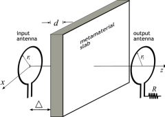
Figure 1: Geometry of a metamaterial lens. The source is a loop antenna located at $z=0$. The detector is also an identical loop antenna. The lens is formed either by a left-handed metamaterial slab or by another planar device that produces SRI through amplification of evanescent harmonics. The output antenna can eventually be loaded with microwave resistors in order to minimize field perturbation.

The present study starts with the canonical problem of the formation of images by a left-handed slab of thickness $d$ characterized by $\epsilon/\epsilon_{0}=\mu/\mu_{0}=-1+i\delta$, where $\delta\ll 1$ accounts for the necessary losses factor to avoid the divergence of field integrals Garcia ; SmithAPL03 ; MarquesMOTL . In our study, and following an usual procedure in microwave SRI experiments, the source will be an antenna (specifically, a loop antenna) whose plane is located parallel to the slab interfaces, as is shown in Fig. 1. The field beyond the lens will be scanned by an output antenna that plays the role of detector. The source here employed is equivalent to an homogeneous surface distribution of magnetic dipoles inside the loop given by $M_{s}=I_{0}\mathrm{e}^{-i\omega t}$, where $I$ denotes the amplitude of the imposed time-harmonic current in the loop. The computation of the longitudinal magnetic field, $H_{z}$, at the image side of the slab ($z>\Delta+d$) can be carried out by means of the following double inverse Fourier transform:

$$H_{z}(x,y,z)=\dfrac{1}{4\pi^{2}}\iint\mathrm{d}k_{x}\mathrm{d}k_{y}\\ \widetilde{G}(k_{x},k_{y};z)\tilde{M}_{s}(k_{x},k_{y})\,\mathrm{e}^{i(k_{x}x+k_{y}y)}\;,$$ (1)

where $\widetilde{G}(k_{x},k_{y};z)$ and $\widetilde{M}_{s}(k_{x},k_{y};z)$ are respectively the Fourier transforms of the Green’s function of the structure under study and of the spatial surface distribution of magnetic dipoles. After applying the duality principle to expression (6) in MarquesMOTL and taking $\Delta=d/2$, the Fourier-transform of the Green’s function is found to be

$$\widetilde{G}(k_{x},k_{y};z)=\dfrac{-k_{t}^{2}2\beta\mathrm{e}^{-i\beta_{0}(z+d)}}{\omega\left\{(\beta\mu_{0}-\beta_{0}\mu)^{2}\mathrm{e}^{i\beta d}-(\beta\mu_{0}+\beta_{0}\mu)^{2}\mathrm{e}^{-i\beta d}\right\}}\;,$$ (2)

with $k_{t}^{2}=(k_{x}^{2}+k_{y}^{2})$ and $\beta=\sqrt{\omega^{2}\varepsilon\mu-k_{t}^{2}}$, $\beta_{0}=\sqrt{\omega^{2}\varepsilon_{0}\mu_{0}-k_{t}^{2}}$. Since $E_{z}=0$ in the present case, the remaining field components can be all deduced from $H_{z}$ MarquesMOTL .

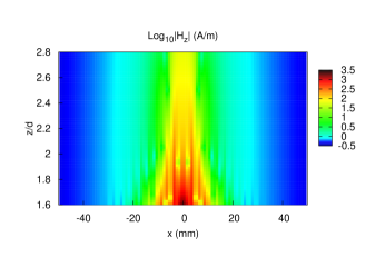
Figure 2: Map of $\log_{10}|H_{z}|$ corresponding to the field generated at the back side of the lens by a source loop antenna shown in Fig. 1. The slab is made of a left-handed medium of thickness $d=4\,$mm with $\epsilon/\epsilon_{0}=\mu/\mu_{0}=-1+i0.001$, and is separated a distance $\Delta=d/2$ from the source. The source is considered, for simplicity, a circular loop antenna of radius $r_{1}=5\,$mm,. The wire radius is of $0.2\,$mm. The operation frequency is 3 GHz.

The numerical computation of (1) provides the map depicted in Fig. 2 for the magnitude of $H_{z}$ in the $(x-z)$ plane at the back side of the lens. It should be noted that, given that the operation frequency is 3 GHz ($\lambda_{0}=100\,$mm) and $d$ and $\Delta$ are taken much less than the free-space wavelength, the ray model approximation cannot be here employed to obtain the fields in the considered region (in other words, we are dealing with near fields and therefore in a SRI situation). According to previous discussions, Fig. 2 shows that the field magnitude has a strong decay along the $z$ direction, so that no information about the location of the source in this direction can be extracted from the field pattern. A more detailed picture of the field distribution at two planes $z=(2\pm\delta)d$ is depicted in Fig. 3 (with $\delta$ set to 0.3), and compared with the field amplitude near the source at $z=\pm\delta d$ (both results are identical).

Figure 3: Plot of the $\log_{10}|H_{z}|$ at different $z$-planes of Fig.1. The slab and the source loop antenna is as in Fig. 2.

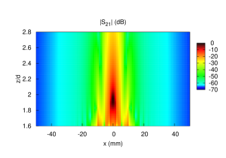
Figure 4: Map of the magnitude in decibels of the transmission coefficient, $|S_{21}|$, between the input and output antennas of Fig. 1. The structural parameters are as in Fig. 2. The output antenna is identical to the input one.

As is expected from the properties of the metamaterial slab, the field distribution at the $z=(2+\delta)d$ plane is almost identical to that at the $z=\delta d$ plane, thus confirming that the $z=\delta d$ and the $z=(2+\delta)d$ planes are in fact conjugate planes. On the contrary, the field distribution at the $z=(2-\delta)d$ plane substantially differs in magnitude from the field distribution at the $z=-\delta$ plane, near the source. These facts corroborate the aforementioned discussions: the super-resolution in the transverse directions (the lateral dimensions of the source and the image are of about one tenth of the wavelength) is compensated by an almost complete loss of resolution in the longitudinal direction.

Next, the problem of the measurement of the image in this SRI experiment will be considered. In the microwave range, the image detection is performed by measuring the transmission coefficient between a source antenna and a receiving antenna, which is scanned in the image side of the lens Houck ; Grbic ; Lagarkov . For simplicity the receiving (or output) antenna will be assumed to be identical to the input antenna employed as source. The transmission coefficient is measured by connecting the input antenna to a wave generator via a waveguide, and the output one to a detector through another identical waveguide (more details of this measurement setup are reported in Freire ). In this approach, the metamaterial slab should be viewed as a matching device Veselago , whose transmission coefficient, $t$ (or $S_{21}$ in the usual microwave terminology), is given by Pozar

$$t=\frac{2Z_{12}Z_{0}}{(Z_{11}+Z_{0})(Z_{22}+Z_{0})-Z_{12}^{2}}\;,$$ (3)

where $Z_{ij}$ are the elements of the impedance matrix for the system formed by the two antennas and the left-handed slab, and $Z_{0}$ is the characteristic impedance of the input/output waveguide. In order to measure a super-resolution image, the size of the loop antennas has to be smaller than the free space wavelength, which additionally would make the real part of $Z_{ij}$ (the radiation resistance Pozar ) be negligible with respect to its imaginary part; namely, $Z_{ij}\simeq-i\omega L_{ij}$, where $L_{ij}$ is the inductance matrix of the system. The diagonal terms of the inductance matrix correspond to the inductances of a single loop antenna faced to the left-handed slab. However, in the “perfect lens” configuration here considered, the slab does not affect the fields around the source Pendry and, therefore, $L_{11}=L_{22}\equiv L$, where $L$ is the self-inductance of the loops in free space. The non-diagonal terms of the inductance matrix account for the mutual inductance of the loop antennas in the presence of the slab, namely $L_{12}=L_{21}\equiv M$. Assuming that the waveguides have a low impedance (typically this impedance is $Z_{0}=50\,\Omega$ for microwave measurements), it will be found that $|Z_{ii}|>Z_{0}$. Thus, neglecting second order terms in $Z_{ii}/Z_{0}$, the transmission coefficient in (3) can be approximated as

$$t\approx\frac{2i\omega MZ_{0}}{\omega^{2}(L^{2}-M^{2})+2i\omega L}\;.$$ (4)

Note that the only spatial dependence in (4) comes from $M$ (since $L$ does not change with the position of the antennas), which causes that the transmission coefficient reaches its maximum ($|t|=1$) at those points where $M\to L$. Since both the input and output antennas are identical, and the field at the source plane is reproduced at the image plane (see Fig. 3), the condition $M\to L$ is expected to be satisfied around the point $(x,y,z)=(0,0,2d)$. In consequence, a maximum of the transmitted power should be detected at this particular point, which thus appears as an “effective focusing point” of the perfect lens.

In order to show the above expected effects in a practical situation, the magnitude of the transmission coefficient has been numerically computed for the configuration under study. The impedance matrix has been calculated by imposing known currents, $I_{i}=1,0\,$A, in the loops, and then computing the corresponding self and mutual inductances. The computation of the self inductance is an standard electromagnetic problem, and the mutual inductance is obtained after computing the flux of the magnetic field given by (1) across the surface of the output antenna. The transmission coefficient is finally determined from (3), assuming $Z_{0}=50\,\Omega$. In Fig. 4 it is shown a map of the computed transmission coefficient for a system composed of two identical lossless loop antennas. It can be observed that this figure substantially differs from Fig. 2; in particular, a clear maximum of $|t|$ can be observed in Fig. 4 in the neighborhood of the image at $(0,0,2d)$. These results clearly show the difference between the transmitted power and the field distribution in the absence of the output antenna, and also how 3D-SRI can be obtained when the appropriate detector is used.

Let us now consider the measurement of the unperturbed field. For this purpose, the detector should be designed to affect the field distribution as less as possible. It could be closely achieved by loading the output antenna with an additional high resistance, which will significantly reduce the current induced at the output antenna, as well as its generated field. In Fig. 5

Figure 5: Magnitude of the computed transmission coefficient along the $Z$ axis between the input and output antennas of Fig. 1 for different resistances loading the output antenna. The structural parameters are as in Fig. 2.

the computed values of the transmission coefficient along the $z$-axis of Fig. 1 are shown for different resistances, $R$, loading the output antenna. As is expected, the curve for $R=0$ shows a maximum near the location of the image, which thus appears as a “focusing point” of the lens, at $z=2d$. (The small difference between the actual location of this maximum and $z=2d$ can be attributed to the non negligible values of the ratio $|Z_{ii}/Z_{0}|\approx 8$ in the problem under study). As is expected, the curves for the highest values of $R$ resemble the behavior of $|H_{z}|$ in Fig. 2 for the unperturbed configuration.

Let us now re-examine the experimental demonstration of 3D-SRI, recently reported in Freire at the light of the above considerations. Although the underlying physics of the device analyzed in Freire is not exactly the same as that of the left-handed perfect lens, both systems show the same process of amplification of evanescent modes and are equivalent in practice for the present purposes. Fig. 6 shows the location of the maximum of the transmission coefficient along the $z$ axis of the magnetoinductive lens reported in Freire , for different values of the resistance loading the output loop. The experimental setup used to obtain these results is described in detail in Freire . The only difference is that, for obtaining the results shown in Fig. 6, the output antenna was loaded by different microwave resistors. A behavior similar to that of Fig. 5 can be observed, thus confirming the proposed theory.

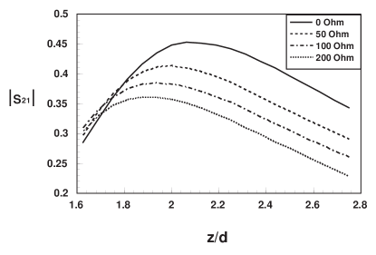
Figure 6: Plots of the measured magnitude of the transmission coefficient between the input and output antennas of Fig. 1 when the slab is substituted by the magneto inductive lens reported in Freire . (Freq=3GHz).

In summary, SRI in metamaterial super-lenses has been investigated. As is well known this imaging is primarily due to the amplification of evanescent modes inside the lens. As a consequence, super-resolution in the planes parallel to the slab is unavoidably compensated by a drastic loss of resolution in the direction perpendicular to the slab. However, since evanescent modes do not carry power, any physical detection (namely, a measurement) of the image at the back side of the lens will require the existence of some amount of transmitted power from the source to the detector, which can significantly affect the field distribution. If this last effect is taken into account, the secondary fields generated by the presence of the detector should be considered. Following this approach, it has been shown that the transmission coefficient between the source and the detector can be made very high. Provided that the appropriate detector is employed (typically a lossless output antenna identical to the input antenna), this maximum will occur in a neighborhood of the image, thus resulting in super-resolution imaging also in the direction perpendicular to the slab. However, it should be emphasized that, to obtain this 3D-SRI some previous knowledge of the source is necessary in order to properly design the detector. Thus, a general conclusion arises from the analysis: Super-resolution in metamaterial super-lenses is always incomplete: if the distance from the source to the lens is known, the shape and characteristics of the source can be recovered without uncertainty from the analysis of the field at the image side of the lens. Conversely, if the shape and characteristics of the source are known, it is possible to design an appropriate detector in order to determine, without uncertainty, the source location in three dimensional space from the transmission coefficient between the source and the detector. However, it is impossible to determine simultaneously, by means of a metamaterial superlens, both the locations and the shape and characteristics of an unknown source wit a resolution overcoming the diffraction limit. We feel that the reported analysis and experiments, as well as the conclusions arising from them, will be of importance in the design of metamaterial super-resolution devices.

References

- (1) V. G. Veselago, Sov. Phys. USPEKHI 10, 509 (1968).
- (2) A.A. Houck, J.B. Brock, I.L. Chuang, Phys. Rev. Lett. 90, 137401 (2003).
- (3) J. B. Pendry, Phys. Rev. Lett. 85, 3966 (2000).
- (4) A. Grbic, G. V. Eleftheriades, Phys. Rev. Lett. 92, 117403 (2004).
- (5) A. N. Lagarkov, V. N. Kissel, Phys. Rev. Lett. 92, 077401 (2004).
- (6) N. Fang, X. Zhang, App. Phys. Lett. 82, 161 (2003).
- (7) M. Freire, R. Marqués, App. Phys. Lett. 86, 182505 (2005).
- (8) J.D. Baena, L. Jelinek, F. Marqués, F. Medina, Phys. Rev. B (accepted)
- (9) N. García, M. Nieto-Vesperinas, Phys. Rev. Lett. 88, 207403 (2002).
- (10) D. R. Smith, D. Schurig, M. Rosenbluth, S. Schultz, S. Anantha Ramakrishna, J. B. Pendry, App. Phys. Lett. 82, 1506 (2003).
- (11) R. Marqués, J. Baena, Microwave and Opt. Tech. Lett. 41, 290 (2004).
- (12) V. G. Veselago, http://xxx.lanl.gov/ftp/cond-mat/papers/0501/0501438.pdf
- (13) D. M. Pozar, Microwave Engineering (J.Wiley & Sons, N.York, 1998), 2nd ed.