Heat transport by turbulent Rayleigh-Bénard Convection in cylindrical samples with aspect ratio one and larger
Abstract
We present high-precision measurements of the Nusselt number as a function of the Rayleigh number for cylindrical samples of water (Prandtl number ) with diameters and 9.2 cm, all with aspect ratio ( is the sample height). In addition, we present data for and and 6. For each sample the data cover a range of a little over a decade of . For they jointly span the range . Where needed, the data were corrected for the influence of the finite conductivity of the top and bottom plates and of the side walls on the heat transport in the fluid to obtain estimates of for plates with infinite conductivity and sidewalls of zero conductivity. For the effective exponent of ranges from 0.28 near to 0.333 near . For the results are consistent with the Grossmann-Lohse model. For larger , where the data indicate that , the theory has a smaller than and falls below the data. The data for are only a few percent smaller than the results.
1 Introduction
A central prediction of theoretical models of turbulent Rayleigh-Bénard convection (RBC) in a fluid heated from below [[Kraichnan(1962), Siggia(1994), Kadanoff(2001), Ahlers, Grossmann & Lohse (2002), Grossmann & Lohse (2000)]] is the dependence of the global heat transport on the Rayleigh number
| (1) |
( is the isobaric thermal expension coefficient, the thermal diffusivity, the kinematic viscosity, the acceleration of gravity, the temperature difference, and the sample height) and the Prandtl number . The heat transport is usually expressed in terms of the Nusselt number
| (2) |
were is the heat-current density and is the thermal conductivity of the fluid in the absence of convection. Before a quantitative comparison between theory and experiment can be made, the results for usually must be corrected for the influence of the side wall [[Ahlers(2000), Roche et al.(2001), Niemela & Sreenivasan (2003)]] and the top and bottom plates [[Chaumat et al.(2002), Verzicco(2004), Brown et al. (2005)]] to yield an estimate of the idealized .
A model developed recently by [Grossmann & Lohse (2000)], based on the decomposition of the kinetic and the thermal dissipation into boundary-layer and bulk contributions, provided a good fit to experimental data [[Xu, Bajaj & Ahlers(2000)], [Ahlers & Xu (2001)]] for a cylindrical sample of aspect ratio ( is the diameter) when it was adapted [[Grossmann & Lohse (2001)], GL] to the relatively small Reynolds numbers of the measurements. However, the data were used to determine four adjustable parameters of the model. Thus more stringent tests using measurements for the same but over wider ranges of and are desirable. A success of the model was the agreement with recent results by [Xia, Lam & Zhou(2002)] for much larger Prandtl numbers than those of [Ahlers & Xu (2001)], for and . It is the primary aim of the present paper to extend the range of over which high-precision data, subject to minimal systematic errors, are available for . Our data span the range with and and deviate from the Boussinesq approximation ([Boussinesq (1903)]) by less than a few tenths of a percent. We believe that they can serve as a benchmark for comparison with future experimental and theoretical developments. They agree quite well with the GL model for , but for larger there are deviations.
In addition to the results for we present also some data for larger , up to . We find that there is remarkably little dependence of on . For instance, the data fall only about 4% below the results.
| No | No | |||||||||||
|---|---|---|---|---|---|---|---|---|---|---|---|---|
| 1 | 40.009 | 1.957 | 94.3 | 127.0 | 129.3 | 2 | 40.011 | 3.911 | 188.6 | 157.5 | 161.4 | |
| 3 | 39.984 | 5.917 | 285.0 | 179.4 | 184.8 | 4 | 40.007 | 7.821 | 377.0 | 195.8 | 202.5 | |
| 5 | 40.007 | 9.764 | 470.7 | 210.1 | 218.0 | 6 | 40.022 | 11.676 | 563.1 | 222.3 | 231.3 | |
| 7 | 40.039 | 13.589 | 655.7 | 233.5 | 243.6 | 8 | 39.955 | 15.688 | 754.8 | 243.7 | 254.9 | |
| 9 | 39.901 | 17.729 | 851.4 | 253.4 | 265.6 | 10 | 39.887 | 19.705 | 945.8 | 261.8 | 274.9 | |
| 11 | 40.041 | 6.783 | 327.3 | 187.5 | 193.5 | 12 | 40.062 | 4.791 | 231.4 | 167.9 | 172.5 | |
| 13 | 40.056 | 2.849 | 137.6 | 142.8 | 145.9 | 14 | 39.963 | 2.543 | 122.4 | 137.5 | 140.3 | |
| 15 | 39.944 | 1.595 | 76.7 | 118.5 | 120.4 | 16 | 39.923 | 19.623 | 943.0 | 261.7 | 274.7 | |
| 17 | 39.921 | 19.627 | 943.2 | 261.6 | 274.7 | 18 | 39.929 | 5.048 | 242.7 | 170.6 | 175.4 | |
| 19 | 39.970 | 1.050 | 50.6 | 104.6 | 106.0 | 20 | 39.999 | 9.775 | 471.1 | 210.3 | 218.2 | |
| 21 | 39.998 | 9.782 | 471.4 | 210.3 | 218.3 | 22 | 40.016 | 0.962 | 46.4 | 101.8 | 103.1 | |
| 23 | 40.015 | 0.963 | 46.4 | 101.9 | 103.2 | 24 | 39.904 | 19.666 | 944.5 | 261.7 | 274.8 | |
| 25 | 39.963 | 2.539 | 122.2 | 137.6 | 140.4 | 26 | 40.000 | 1.485 | 71.5 | 116.3 | 118.1 | |
| 27 | 40.011 | 1.954 | 94.2 | 127.0 | 129.2 | 28 | 40.011 | 1.955 | 94.3 | 126.9 | 129.2 | |
| 29 | 40.010 | 1.954 | 94.2 | 126.9 | 129.1 | 30 | 39.993 | 1.005 | 48.4 | 103.1 | 104.4 | |
| 31 | 39.859 | 21.687 | 1040.0 | 269.4 | 283.3 | 32 | 39.971 | 3.988 | 192.0 | 158.4 | 162.4 |
| No | No | |||||||||||
|---|---|---|---|---|---|---|---|---|---|---|---|---|
| 1 | 39.985 | 2.002 | 11.3 | 66.5 | 66.6 | 2 | 40.014 | 2.437 | 13.7 | 70.5 | 70.6 | |
| 3 | 40.003 | 3.147 | 17.7 | 76.0 | 76.2 | 4 | 39.968 | 4.005 | 22.6 | 81.7 | 81.9 | |
| 5 | 39.987 | 4.951 | 27.9 | 87.2 | 87.5 | 6 | 39.973 | 6.202 | 34.9 | 93.3 | 93.7 | |
| 7 | 39.994 | 7.679 | 43.3 | 99.6 | 100.1 | 8 | 39.946 | 9.731 | 54.8 | 107.0 | 107.6 | |
| 9 | 39.956 | 11.862 | 66.8 | 113.7 | 114.5 | 10 | 39.928 | 14.259 | 80.2 | 120.3 | 121.2 | |
| 11 | 39.911 | 16.824 | 94.6 | 126.5 | 127.6 | 12 | 39.865 | 19.836 | 111.3 | 133.1 | 134.5 | |
| 13 | 39.979 | 1.618 | 9.1 | 62.4 | 62.5 | 14 | 39.998 | 1.282 | 7.2 | 58.3 | 58.3 | |
| 15 | 39.970 | 1.041 | 5.9 | 54.8 | 54.9 | 16 | 39.968 | 0.845 | 4.8 | 51.6 | 51.6 | |
| 17 | 39.967 | 0.650 | 3.7 | 47.7 | 47.7 | 18 | 39.989 | 0.507 | 2.9 | 44.4 | 44.5 | |
| 19 | 39.954 | 22.581 | 127.1 | 138.7 | 140.2 | 20 | 39.959 | 23.539 | 132.6 | 140.4 | 142.0 | |
| 21 | 39.948 | 25.499 | 143.5 | 143.9 | 145.6 | 22 | 39.942 | 28.420 | 159.9 | 148.7 | 150.7 | |
| 23 | 39.943 | 31.330 | 176.3 | 153.2 | 155.4 | 24 | 39.936 | 34.193 | 192.4 | 157.4 | 159.7 | |
| 25 | 39.944 | 37.110 | 208.9 | 161.2 | 163.7 | 26 | 39.960 | 39.968 | 225.1 | 164.8 | 167.5 |
| No | No | |||||||||||
|---|---|---|---|---|---|---|---|---|---|---|---|---|
| 1 | 39.995 | 0.571 | 18.46 | 20.68 | 20.33 | 2 | 39.995 | 0.721 | 23.34 | 22.13 | 21.76 | |
| 3 | 39.995 | 0.914 | 29.58 | 23.86 | 23.47 | 4 | 39.995 | 1.160 | 37.53 | 25.51 | 25.11 | |
| 5 | 39.995 | 1.473 | 47.64 | 27.35 | 26.94 | 6 | 39.995 | 1.871 | 60.52 | 29.28 | 28.86 | |
| 7 | 39.995 | 2.378 | 76.92 | 31.31 | 30.91 | 8 | 39.995 | 3.025 | 97.85 | 33.57 | 33.13 | |
| 9 | 39.995 | 3.846 | 124.44 | 35.93 | 35.50 | 10 | 39.996 | 4.894 | 158.35 | 38.44 | 38.00 | |
| 11 | 39.996 | 6.229 | 201.52 | 41.17 | 40.71 | 12 | 39.996 | 7.927 | 256.49 | 44.02 | 43.55 | |
| 13 | 39.998 | 10.092 | 326.53 | 47.08 | 46.60 | 14 | 39.999 | 12.848 | 415.73 | 50.35 | 49.87 | |
| 15 | 39.999 | 16.357 | 529.28 | 53.97 | 53.49 | 16 | 40.002 | 20.823 | 673.87 | 57.80 | 57.30 | |
| 17 | 40.035 | 26.550 | 860.19 | 61.92 | 61.41 | 18 | 40.054 | 33.658 | 1091.23 | 66.23 | 65.71 | |
| 19 | 40.025 | 33.727 | 1092.34 | 66.37 | 65.85 | 20 | 40.021 | 35.710 | 1156.37 | 67.41 | 66.90 | |
| 21 | 40.051 | 37.630 | 1219.84 | 68.45 | 67.93 | 22 | 40.080 | 39.579 | 1284.33 | 69.41 | 68.90 | |
| 1 | 39.996 | 0.636 | 20.58 | 21.23 | 20.88 | 2 | 39.996 | 1.026 | 33.21 | 24.44 | 24.06 | |
| 3 | 39.997 | 1.660 | 53.70 | 28.13 | 27.72 | 4 | 39.999 | 2.691 | 87.08 | 32.23 | 31.81 | |
| 5 | 40.002 | 4.348 | 140.72 | 37.00 | 36.56 | 6 | 40.007 | 7.044 | 227.98 | 42.43 | 41.98 | |
| 7 | 40.008 | 11.433 | 370.05 | 48.69 | 48.19 | 8 | 40.018 | 18.527 | 599.87 | 55.89 | 55.39 | |
| 9 | 40.049 | 30.001 | 972.45 | 64.19 | 63.68 | 10 | 40.065 | 39.567 | 1283.28 | 69.68 | 69.16 |
| No | No | |||||||||||
|---|---|---|---|---|---|---|---|---|---|---|---|---|
| 1 | 39.901 | 17.562 | 233.67 | 164.7 | 172.6 | 2 | 40.012 | 15.429 | 206.09 | 158.5 | 165.7 | |
| 3 | 39.898 | 13.727 | 182.62 | 152.6 | 159.2 | 4 | 39.986 | 11.633 | 155.24 | 145.1 | 151.0 | |
| 5 | 39.956 | 9.763 | 130.14 | 137.4 | 142.6 | 6 | 39.959 | 7.837 | 104.48 | 128.4 | 132.8 | |
| 7 | 40.089 | 5.663 | 75.85 | 116.2 | 119.7 | 8 | 39.984 | 3.928 | 52.42 | 103.6 | 106.2 | |
| 9 | 40.010 | 1.939 | 25.90 | 83.5 | 85.0 | 10 | 39.970 | 1.041 | 13.88 | 69.3 | 70.2 | |
| 11 | 39.959 | 3.006 | 40.08 | 95.4 | 97.5 | 12 | 40.031 | 4.803 | 64.19 | 110.3 | 113.3 | |
| 13 | 40.252 | 6.302 | 84.89 | 120.4 | 124.2 | 14 | 39.905 | 17.563 | 233.71 | 164.6 | 172.4 | |
| 15 | 39.944 | 8.837 | 117.75 | 132.9 | 137.7 | |||||||
| 1 | 39.822 | 19.669 | 260.43 | 170.5 | 179.1 | 2 | 39.827 | 17.730 | 234.80 | 165.3 | 173.3 | |
| 3 | 40.025 | 13.517 | 180.25 | 152.1 | 158.6 | 4 | 41.676 | 12.258 | 172.99 | 150.4 | 156.8 | |
| 5 | 40.083 | 7.623 | 101.86 | 127.5 | 131.8 | 6 | 39.973 | 5.900 | 78.53 | 117.6 | 121.2 | |
| 7 | 40.005 | 3.901 | 51.98 | 103.5 | 106.1 | 8 | 40.008 | 1.948 | 25.96 | 83.6 | 85.1 | |
| 9 | 40.051 | 2.838 | 37.88 | 93.8 | 95.8 |
| No | No | |||||||||||
|---|---|---|---|---|---|---|---|---|---|---|---|---|
| 1 | 40.012 | 1.944 | 1097.6 | 63.86 | 65.06 | 2 | 39.993 | 3.932 | 2218.8 | 79.11 | 81.17 | |
| 3 | 40.104 | 5.660 | 3206.3 | 88.60 | 91.31 | 4 | 39.982 | 7.846 | 4426.2 | 97.92 | 101.37 | |
| 5 | 39.981 | 9.789 | 5521.8 | 104.75 | 108.79 | 6 | 40.034 | 11.626 | 6570.7 | 110.63 | 115.22 | |
| 7 | 39.929 | 13.777 | 7757.4 | 116.43 | 121.58 | 8 | 39.483 | 14.643 | 8116.3 | 117.92 | 123.23 | |
| 9 | 39.977 | 10.767 | 6072.7 | 107.91 | 112.24 | 10 | 40.056 | 6.732 | 3807.7 | 93.38 | 96.47 | |
| 11 | 40.045 | 4.802 | 2715.1 | 84.25 | 86.66 | 12 | 39.966 | 3.011 | 1697.7 | 72.74 | 74.41 | |
| 13 | 39.972 | 1.041 | 587.2 | 52.83 | 53.55 | 14 | 39.961 | 17.593 | 9917.0 | 125.58 | 131.70 |
| No | No | |||||||||||
|---|---|---|---|---|---|---|---|---|---|---|---|---|
| 1 | 39.990 | 17.576 | 2937.8 | 85.32 | 89.59 | 2 | 40.007 | 17.578 | 2939.7 | 85.40 | 89.68 | |
| 3 | 40.100 | 15.454 | 2592.9 | 82.13 | 86.04 | 4 | 39.974 | 13.743 | 2295.8 | 79.17 | 82.76 | |
| 5 | 40.062 | 11.622 | 1947.5 | 75.26 | 78.47 | 6 | 39.978 | 9.839 | 1643.8 | 71.42 | 74.26 | |
| 7 | 40.030 | 5.839 | 977.3 | 60.99 | 62.94 | 8 | 40.002 | 3.928 | 656.9 | 54.02 | 55.48 | |
| 9 | 40.016 | 1.941 | 324.7 | 43.75 | 44.61 | 10 | 39.974 | 1.040 | 173.8 | 36.41 | 36.94 | |
| 11 | 40.063 | 2.830 | 474.2 | 48.99 | 50.14 | 12 | 40.054 | 4.807 | 805.2 | 57.47 | 59.17 | |
| 13 | 40.283 | 6.311 | 1065.7 | 62.65 | 64.74 | 14 | 39.987 | 8.846 | 1478.4 | 69.18 | 71.82 |
| No | No | |||||||||||
|---|---|---|---|---|---|---|---|---|---|---|---|---|
| 1 | 40.000 | 19.734 | 412.4 | 46.09 | 48.62 | 2 | 39.977 | 17.804 | 371.8 | 44.74 | 47.11 | |
| 3 | 39.402 | 16.991 | 347.7 | 43.83 | 46.09 | 4 | 40.134 | 13.567 | 284.9 | 41.32 | 43.31 | |
| 5 | 40.058 | 11.727 | 245.6 | 39.58 | 41.37 | 6 | 40.054 | 9.781 | 204.8 | 37.51 | 39.10 | |
| 7 | 40.137 | 7.637 | 160.4 | 34.95 | 36.30 | 8 | 40.015 | 5.920 | 123.8 | 32.38 | 33.51 | |
| 9 | 40.032 | 3.909 | 81.8 | 28.73 | 29.57 | 10 | 40.019 | 1.944 | 40.7 | 23.62 | 24.14 | |
| 11 | 40.071 | 2.839 | 59.5 | 26.26 | 26.94 | 12 | 40.085 | 4.791 | 100.4 | 30.49 | 31.47 | |
| 13 | 40.070 | 6.800 | 142.5 | 33.72 | 34.96 | 14 | 40.051 | 3.375 | 70.7 | 27.55 | 28.31 |
2 Problems associated with high-precision measurements of
One problem in the measurements of is that data with a precision of 0.1% or so can be obtained in a given sample only over a range of covering a little more than a decade unless the fluid is changed. The reason is that the useful temperature differences with conventional fluids like water are limited at the high end to C by possible contributions from non-Boussinesq effects ([Boussinesq (1903)]) and at the low end to C by thermometer resolution. For this reason we built three apparatus containing samples of diameter and 9.2 cm, all with and known as the large, medium, and small apparatus or sample respectively ([Brown et al. (2005)]). Together the data obtained with these span the range .
A second experimental problem is the influence of the side wall on the heat transport by the fluid ([Ahlers(2000), Roche et al.(2001), Niemela & Sreenivasan (2003)]). Because of the nonlinear temperature profile in the wall adjacent to the thermal boundary layers in the fluid, the heat entering (leaving) the wall at the bottom (top) can be much larger than an estimate based on a constant temperature gradient. In the present work we substantially reduced this problem by choosing a wall of small conductivity (plexiglas or lexan) and a fluid of relatively large conductivity (water). An estimate [model 2 of [Ahlers(2000)]] indicated that the side-wall corrections for the large and medium samples were less than a few tenths of a percent; they were neglected. For the small sample the correction was 1.7% for and smaller at larger , and was made [[Brown et al. (2005)]] using model 2 of [Ahlers(2000)]. We believe that for all the data the systematic errors due to the side-wall correction is significantly less than one percent.
A third problem is the effect of the finite conductivity of the confining top and bottom plates on the heat transport by the fluid [[Chaumat et al.(2002), Verzicco(2004), Chillà et al.(2004a)]]. We investigated this effect experimentally [[Brown et al. (2005)]] by making measurements for samples of different sizes and aspect ratios, each with copper plates ( W/m K) and with aluminum plates ( W/m K). For the large and medium apparatus a small difference between the data sets enabled us to derive a correction factor. When applied to the data taken with the copper plates it yielded an increase of less than 5% for the large and less than 1% for the medium apparatus and gave a good estimate of the idealized . For the small apparatus the results obtained with copper and aluminum plates agreed with each other.
3 Results
3.1 The data
The measurements were made at a mean temperature of 40∘C, where m2/s, m2/s, K-1, and W/m K. We never observed long transients like those reported by [Chillà et al.(2004b)] for (see [Brown et al. (2005)]). On occasion we tilted the apparatus by 2∘, and within our resolution of 0.1% found no effect on .
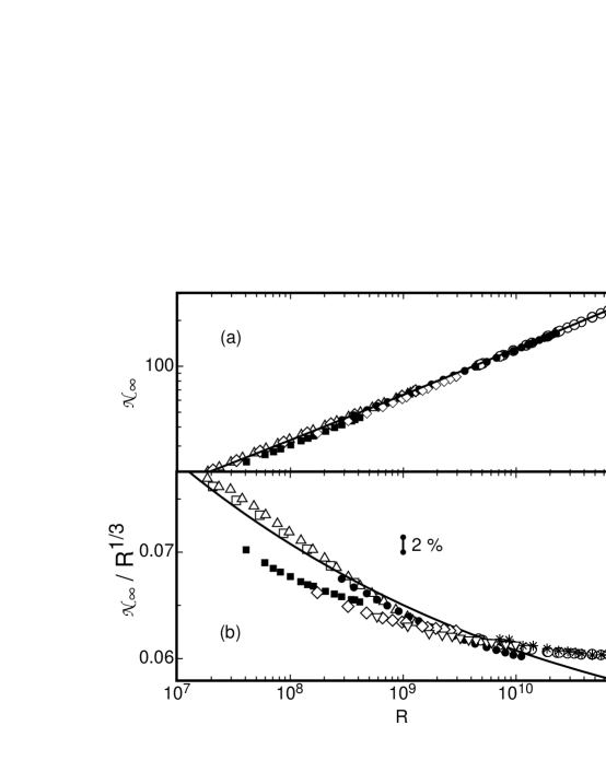
The results for and are given in Tables 1 to 7 and are shown on logarithmic scales in Fig. 1a. With greater resolution they are shown in the compensated form in Fig. 1b. The results for in Table 1 are not the same as those reported previously (run 1, [Nikolaenko et al. (2005)] Table 4; those results for and should be reduced by 0.5% because of an error in the area used in the original data analysis). They were taken in a second experiment (run 2) after the sample had been taken apart and re-assembled. Likewise, there are two separate runs for in the small apparatus (Table 3) and for in the large apparatus (Table 4). Within a given run the measurements were reproducible within one or two tenths of a percent (see, for instance, points 17 and 24 in Table 1). The two runs for (Table 4) agree within their scatter of about 0.1%. On the other hand, the two runs with the large apparatus for (Table 1 and [Nikolaenko et al. (2005)] Table 4), as well as the two runs from the small apparatus (Table 3), differ from each other by a few tenths of a percent, but by no more than expected possible systematic errors.
The results for from the small, medium, and large samples fall on nearly continuous smooth curves, but close inspection shows that there are small systematic offsets. The data lie close to the GL model (solid line). It is remarkable that the data come so close to the results. For instance, the values are only about 4% below the measurements. One assumes that the large- sample had a much more complex large-scale-flow structure than the single circulating roll expected to exist for . Apparently this has only a very modest influence on the heat transport.
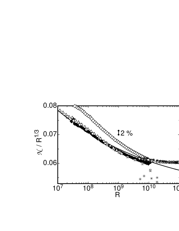
In Fig. 2 we compare the present results with previous measurements for and close to 4. Data for obtained using acetone () are shown as open diamonds [[Xu, Bajaj & Ahlers(2000)]]. The corresponding results obtained after a correction for the side-wall conductance [model 2, [Ahlers(2000)]] are given as solid diamonds. One sees that in this case the wall correction is quite large, reaching about 8 % for (no plate correction was required in this case, see [Brown et al. (2005)]). Nonetheless the corrected data for are in excellent overall agreement with the present results. The open squares with solid dots at their centers represent the results of [Xia, Lam & Zhou(2002)] using water with . Up to they agree extremely well with the present measurements. For larger they are slightly lower, presumably because of the influence of the finite plate conductivity. Also shown are data from [Goldstein & Tokuda (1979)]. When corrections for the finite plate-conductivity (which had not been made) and the difference in are considered, they may be regarded as consistent with the present results.
| 0.0921 | 16.55 | 0.1160 | 17.70 | 0.1464 | 18.95 | 0.1846 | 20.27 | 0.2334 | 21.69 |
| 0.2958 | 23.40 | 0.3753 | 25.04 | 0.4764 | 26.86 | 0.6052 | 28.78 | 0.7692 | 30.79 |
| 0.9785 | 33.04 | 1.2440 | 35.39 | 1.5830 | 37.86 | 2.0150 | 40.59 | 2.5650 | 43.42 |
| 3.2650 | 46.46 | ||||||||
| 0.1285 | 18.63 | 0.2058 | 21.23 | 0.3321 | 24.44 | 0.5370 | 28.13 | 0.8708 | 32.23 |
| 1.4070 | 37.00 | 2.2800 | 42.43 | 3.7010 | 48.69 | ||||
| 2.857 | 44.72 | 3.661 | 48.00 | 4.763 | 51.95 | 5.864 | 55.19 | 7.227 | 58.66 |
| 9.119 | 62.88 | 11.283 | 66.96 | 13.749 | 71.07 | 17.749 | 76.66 | 22.561 | 82.44 |
| 27.906 | 88.01 | 34.944 | 94.29 | 43.297 | 100.67 | 54.777 | 108.30 | 66.792 | 115.21 |
| 66.792 | 115.21 | ||||||||
| 46.36 | 102.79 | 46.42 | 102.90 | 48.42 | 104.11 | 50.55 | 105.63 | 71.55 | 117.77 |
| 76.73 | 120.02 | 94.20 | 128.84 | 94.20 | 128.75 | 94.26 | 128.78 | 94.33 | 128.87 |
| 122.18 | 139.94 | 122.39 | 139.84 | 137.57 | 145.40 | 188.56 | 160.89 | 192.00 | 161.87 |
| 231.37 | 172.01 | 242.66 | 174.83 | 284.99 | 184.23 | 327.32 | 192.89 | 376.98 | 201.89 |
| 470.65 | 217.34 | 471.05 | 217.50 | 471.35 | 217.56 | 563.10 | 230.58 | 655.73 | 242.84 |
| 655.73 | 242.84 |
3.2 Strictly Boussinesq data for
The influence of departures from the Oberbeck-Boussinesq approximation (OBA) [[Boussinesq (1903)]] was considered by various authors. Most recently [Niemela & Sreenivasan (2003)] (NS) examined the issue in considerable detail in terms of various fluid properties. Unfortunately at present we have no theoretical criteria to decide whether a given variation over the applied temperature difference of a given property will affect significantly. Here we provide some insight into this problem from measurements with samples of different sizes but the same .
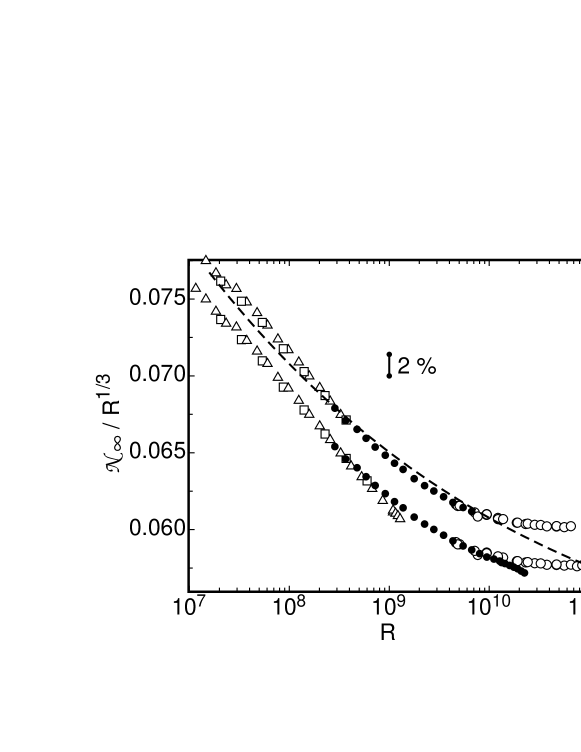
Where they overlap, there is a small systematic offset between the data from the small sample, run 2 on the one hand and the medium-sample on the other. A similar offset exists between the data from the medium sample, and the large sample run 2. These offsets are well within possible experimental systematic errors. In order to obtain a single internally consistent data set spanning the entire range , we shifted the data for from the small sample, run 2 downward by 0.3%. We also shifted the medium-sample data upward by 0.6%, and those from the large sample, run 2 downward by 0.3%. The result is shown by the lower sets of data (displaced downward by 0.0025 for clarity) in Fig. 3. The results from all three samples now merge smoothly into each other. We can then attribute the deviations of the small-sample data at their largest values of from the medium-sample data to deviations from the OBA. A similar situation prevails with respect to the deviations of the medium-sample data from the large-sample results for .
The upper sets of data in Fig. 3 (plotted without any vertical shift) consist only of those points, taken from the lower sets, that fall within approximately 0.2% of a smooth, continuous line through all the results. In Table 8 we give these points in numerical form. We regard these results as conforming “strictly” to the OBA. They are our best estimate of for and , and constitute the primary result of our work.
3.3 The effective exponent of
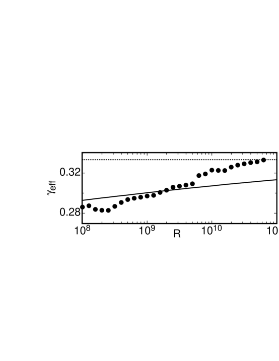
A powerlaw was fit to the data for in the strictly Boussinesq range (Table 8) within a sliding window covering half a decade of . The results for are shown in Fig. 4. Near one sees that has a value close to , the result of early theories (see, for instance, [Siggia(1994)]). With increasing it increases linearly with within experimental error, reaching the large- asymptotic value of the GL model at the finite value . Precision measurements conforming to the OBA for and a wider range of above are needed to determine whether will remain at 1/3.
As was seen in Fig. 3, the GL model is in reasonable agreement with the experimental results for up to . However, for the model increases somewhat more slowly with (solid line in Fig. 4) and reaches 1/3 only in the limit as whereas the experimental becomes equal to 1/3 at the finite .
The result was obtained before by [Goldstein & Tokuda (1979)]. However, they simultaneously fitted all their data, regardless of , over the range to a power law, and found over the entire range. This is not in agreement with our results for which yield an -dependent .
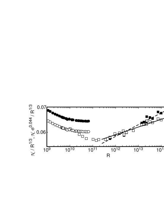
An exponent close to 1/3 was found also by NS in experiments for using helium gas where changed with from about 1 to about 3.8. Those data (open squares) are displayed together with ours (open circles) in Fig. 5. Over the range they can be represented by a powerlaw with (solid line) (when only data for are fitted, one obtains ). The -dependence of at constant is not known very well. For , , and we have [[Nikolaenko et al. (2005)]]. In order to see how much this could possibly influence the -dependence, we also fitted the NS data for (solid squares) and obtained (dashed line). The results by NS, together with ours, suggest that increases beyond 1/3 as grows beyond .
4 Acknowledgment
This work was supported by the US Department of Energy through Grant DE-FG02-03ER46080.
References
- [Ahlers(2000)] Ahlers, G. 2000 Effect of Sidewall Conductance on Heat-Transport Measurements for Turbulent Rayleigh-Benard Convection. Phys. Rev. E 63, 015303-1–4(R).
- [Ahlers, Grossmann & Lohse (2002)] Ahlers, G., Grossmann, S. & Lohse, D. 2002 Hochpräzision im Kochtopf: Neues zur turbulenten Konvektion. Physik Journal 1 (2), 31–37.
- [Ahlers & Xu (2001)] Ahlers, G. & Xu, X. 2001 Prandtl number dependence of heat transport in turbulent Rayleigh-Bénard convection. Phys. Rev. Lett 86, 3320–3323.
- [Boussinesq (1903)] Boussinesq, J. 1903 Théorie Analytique de la Chaleur (Gauthier-Villars, Paris).
- [Brown et al. (2005)] Brown, E., Nikolaenko, A., Funfschilling, D., & Ahlers, G. 2005 Heat transport in turbulent Rayleigh-Bénard convection: Effect of finite top- and bottom-plate conductivity. Submitted to Phys. Fluids.
- [Chaumat et al.(2002)] Chaumat, S., Castaing, B., & Chillà, F. 2002 Rayleigh-Bénard cells: influence of the plates properties Advances in Turbulence IX, Proceedings of the Ninth European Turbulence Conference, edited by I.P. Castro and P.E. Hancock (CIMNE, Barcelona) .
- [Chillà et al.(2004a)] Chillà, F., Rastello, M., Chaumat, S., & Castaing, B. 2004a Ultimate regime in Rayleigh-Bénard convection: The role of the plates. Phys. Fluids 16, 2452–2456.
- [Chillà et al.(2004b)] Chillà, F., Rastello, M., Chaumat, S., & Castaing, B. 2004b Long relaxation times and tilt sensitivity in Rayleigh-Bénard turbulence. Euro. Phys. J. B 40, 223–227.
- [Goldstein & Tokuda (1979)] Goldstein, R.J. & Tokuda, S. 1979 Heat transfer by thermal convection at high Rayleigh numbers. Int. J. Heat Mass Transfer 23, 738–740.
- [Grossmann & Lohse (2000)] Grossmann, S. & Lohse, D. 2000 Scaling in thermal convection: A unifying view. J. Fluid Mech. 407, 27–56.
- [Grossmann & Lohse (2001)] Grossmann, S. & Lohse, D. 2001 Thermal convection for large Prandtl number. Phys. Rev. Lett. 86, 3317–3319.
- [Grossmann & Lohse (2002)] Grossmann, S. & Lohse, D. 2002 Prandtl and Rayleigh number dependence of the Reynolds number in turbulent thermal convection. Phys. Rev. E. 66, 016305.
- [Grossmann & Lohse (2003)] Grossmann, S. & Lohse, D. 2003 On geometry effects in Rayleigh-Bénard convection. J. Fluid Mech. 486, 105–114.
- [Grossmann & Lohse (2004)] Grossmann, S. & Lohse, D. 2004 Fluctuations in turbulent Rayleigh-Bénard convection: the role of plumes. Phys. Fluids 16, 4462–4472.
- [Kadanoff(2001)] Kadanoff, L. P. 2001 Turbulent heat flow: Structures and scaling. Phys. Today 54 (8), 34–39.
- [Kraichnan(1962)] Kraichnan, R. 1962 Turbulent thermal convection at arbitrary Prandtl number. Phys. Fluids 5, 1374–1389.
- [Niemela & Sreenivasan (2003)] Niemela, J. & Sreenivasan, K. R. 2003 Confined turbulent convection. J. Fluid Mech. 481, 355–384.
- [Nikolaenko & Ahlers (2003)] Nikolaenko, A. & Ahlers, G. 2003 Nusselt number measurements for turbulent Rayleigh-Bénard convection. Phys. Rev. Lett 91, 084501-1–4.
- [Nikolaenko et al. (2005)] Nikolaenko, A. , Brown, E., Funfschilling, D., & Ahlers, G. 2005 Heat transport by turbulent Rayleigh-Bénard Convection in cylindrical cells with aspect ratio one and less. J. Fluid Mech. 523, 251–260.
- [Roche et al.(2001)] Roche, P., Castaing, B., Chabaud, B., Hebral, B., & Sommeria, J. 2001 Side wall effects in Rayleigh-Bénard experiments. Europhys. J. B 24, 405–408.
- [Siggia(1994)] Siggia, E. D. 1994 High Rayleigh number convection. Annu. Rev. Fluid Mech. 26, 137–168.
- [Verzicco(2002)] Verzicco, R. 2002 Side wall finite-conductivity effects in confined turbulent thermal convection. J. Fluid Mech. 473, 201–210.
- [Verzicco(2004)] Verzicco, R. 2004 Effects of non-perfect thermal sources in turbulent thermal convection. Phys. Fluids 16, 1965–1979.
- [Verzicco & Camussi(2003)] Verzicco, R. &Camussi, R. 2003 Numerical experiments on strongly turbulent thermal convection in a slender cylindrical cell. J. Fluid Mech. 477, 19–49.
- [Xia, Lam & Zhou(2002)] Xia, K.-Q., Lam, S. & Zhou, S.-Q. 2002 Heat-flux measurements in high-Prandtl-number Rayleigh-Bénard convection. Phys. Rev. Lett. 88, 064501-1–4.
- [Xu, Bajaj & Ahlers(2000)] Xu, X., Bajaj, K. M. S. & Ahlers, G. 2000 Heat transport in turbulent Rayleigh-Bénard convection. Phys. Rev. Lett. 84, 4357–4360.