Improvement of speech recognition by nonlinear noise reduction

Abstract

The success of nonlinear noise reduction applied to a single channel recording of human voice is measured in terms of the recognition rate of a commercial speech recognition program in comparison to the optimal linear filter. The overall performance of the nonlinear method is shown to be superior. We hence demonstrate that an algorithm which has its roots in the theory of nonlinear deterministic dynamics possesses a large potential in a realistic application.

It is a common nuisance that in signal recording, signal transmission, and signal storage, perturbations occur which distort the original signal. In many cases these perturbations are purely additive, so that in principle they could be removed once identified. If these perturbations are sufficiently uncorrelated and appear to be random, they are called noise. Noise reduction is hence an important data processing task. Traditionally, the distinction between signal and noise is done in the frequency domain, where noise contributes with a broad background to a signal which should occupy distinguished frequency bands only. If the signal itself is irregular in time and hence has a broad power spectrum, spectral methods have a poor performance. Nonlinear methods for noise reduction assume and exploit constraints in the clean signal which are beyond second order statistics and hence are most efficiently captured by non-parametric dynamical modelling of the signal. In this paper it is shown that a particular such algorithm is able to denoise a recorded human voice signal so that the recognition rate of a commercial speech recognition program is significantly enhanced. Hence, we have not only a more suitable quantifier for the success of noise reduction on human voice, but we also verify that noise reduction algorithms do what they should do, namely enhance the intelligibility of the signal. This latter aspect is highly non-trivial, since every noise reduction algorithm when removing noise also distorts the signal. Finding merely a positive gain hence does not guarantee that a human (or algorithm) really understands better the meaning of the signal.

I Introduction

Noise reduction and source separation are ubiquitous data analysis and signal processing tasks. In the analysis of chaotic data, noise reduction became a prominent issue about 15 years ago Schreiber1 ; kostelich ; Schreiber2 ; Farmer ; hammel ; davies ; Hsu ; Sauer ; GHKSS . Since the analysis of chaotic data in terms of dimensions, entropies and Lyapunov exponents requires an access to the small length scales (small scale fluctuations of the signal), already a moderate amount of measurement noise on data is known to be destructive. On the other hand, a deterministic source of a signal, albeit potentially chaotic, supplies redundancy which enables one to distinguish between signal and noise and eventually to remove the latter to some extend. Noise reduction schemes which exploit such dynamical constraints were proposed in Schreiber1 ; kostelich ; Schreiber2 ; Farmer ; hammel ; davies ; Hsu ; Sauer ; GHKSS and where tested on many data sets. Since such algorithms were designed to treat chaotic data, they do not make use of spectral properties of data and can, in principle, even remove in-band noise, which is noise whose high frequency spectrum is identical to the spectrum of the signal.

Human voice is a typical non-stationary signal, where noise reduction is a relevant issue. In telecommunication, in the development of hearing aids, and in automatic speech recognition, noise contamination of the speech signal poses severe problems. In multiple simultaneous recordings, noise reduction is also known as blind source separation. However, most often a single recording only is available. In a previous study kantzhuman ; IEEE we demonstrated that nonlinear noise reduction can cope with noise on human speech data and has a performance, which is comparable to advanced spectral adaptive filter banks. The main differences in concepts of linear and nonlinear methods of noise reduction used in this paper are listed in Table 1.

The performance of a noise reduction scheme is usually measured as gain in dB. For this purpose, one starts with a clean signal $\tilde{x}(t)$, numerically adds noise to $\tilde{x}(t)$ resulting in $x(t)$, and then applies the noise reduction scheme without making use of $\tilde{x}(t)$. When we call the result of the noise reduction $y(t)$, then the gain is defined as the logarithm of the ratio of the noise power before and after the noise reduction, which is

$$\mbox{gain}=10\log_{10}\left(\frac{\langle(x(t)-\tilde{x}(t))^{2}\rangle}{\langle(y(t)-\tilde{x}(t))^{2}\rangle}\right)\;,$$ (1)

where $\langle\ldots\rangle$ indicate the time average. This quantity has three drawbacks, namely i) it cannot be computed without knowledge of the clean signal $\tilde{x}(t)$, ii) it can be negative if the initial noise level is low, since distortion of the signal by the filter can be stronger than the reduction of noise, and iii) it does not quantify whether the intelligibility of the signal was improved by the noise reduction. The latter is easily seen by considering the limit of a very high noise level: in such a case setting $y(t)=0\;\;\forall t$ will yield a positive gain, even if this completely eliminates the signal. Therefore, we employ in this paper a commercial speech recognition program as a quantifier of the success of noise reduction. The relative number of words which are not correctly recognized is taken as a quantifier for the signal corruption, regardless of whether this is noise or some systematic distortion which might be introduced by the noise reduction scheme.

In this paper we briefly recall the algorithm including its adaptation for the treatment of voice data, which are nonstationary limit cycle-like signals with embedded noisy segments (stemming from the fricatives). We then apply it to data samples which without added noise are perfectly recognized by the speech recognition software. We demonstrate that our optimised noise reduction scheme does not reduce the recognition rate when it is applied to clean data, and that it improves the recognition rate when it is applied to noisy data, which is comparable with a reduction of the noise amplitude by about 1/2. Noise level $\%N$ is defined as 100 times the ratio of the standard deviation of noise $\sigma$ and standard deviation of data $\sigma_{data}$: $\%N=100\cdot\sigma/\sigma_{data}$.

Table 1: The conceptional comparison between linear methods, LP methods and Hybrid method.

Methods/	Linear methods	Nonlinear methods	Hybrid methods
Concepts	(eg. low pass filter)	(eg. GHKSS)	(eg. LPNCF)
Finding	in time	in space	in time
neighbours			and in space
Finding	smoothing	smoothing	smoothing
corrections	in time	in phase space	using the information
			in time and in space
Noise	in Fourier	violation	violation
estimation	space	of constraints	of constraints
		in phase space	in time and in space

II Method

For the purposes of noise reduction (NR) in voice signals we use the LPNCF urbnrflow and the GHKSS method GHKSS for comparison. The GHKSS method is one version of the Local Projective (LP) Schreiber1 ; kostelich ; Schreiber2 ; Farmer ; hammel ; davies ; Hsu ; Sauer ; GHKSS method that was developed for chaotic signals corrupted by noise. Assuming that the clean data are confined to some deterministic attractor in a reconstructed state space, which itself is locally a subset of a smooth manifold, the method aims at identifying this local manifold in linear approximation and to project the noisy state vector (which due to noise is not confined to this hyperplane) onto the local manifold. Algorithmically, this means to identify a neighbourhood in the delay embedding space and to perform a Singular Value Decomposition of a particular covariance matrix. Some refinements are described in GHKSS .

The LPNCF method, which was particularly developed for chaotic flows, makes use of nonlinear constraints which appear because of the time continuous character of the flow. These constraints are functionals of the state vectors which assume the value $0$ for dense sampling of deterministic data. Let $\left\{x_{i}\right\}$ for $i=1,2,\ldots,N$ be the time series. We denote the corresponding clean signal by $\left\{\tilde{x}_{i}\right\}$, so with the measurement noise $\left\{\eta_{i}\right\}$ we have $x_{i}=\tilde{x}_{i}+\eta_{i}$ for $i=1,2,\ldots,N$. We define the time delay vectors $\mathbf{x}_{i}=(x_{i},x_{i-1},\ldots,x_{i-(d-1)})$ as our points in the reconstructed phase space. Then we choose two neighbours $\mathbf{x}_{k},\mathbf{x}_{j}\in\mathbf{X}_{n}^{NN}$ of the vector $\mathbf{x}_{n}$ ($\mathbf{X}_{n}^{NN}$ is the set neighbours of the point $\mathbf{x}_{n}$). Let us introduce the following function urbnr03

$$G_{n}(s)=x_{n-s}\left(x_{k+1-s}-x_{j+1-s}\right)$$

$$+x_{k-s}\left(x_{j+1-s}-x_{n+1-s}\right)+x_{j-s}\left(x_{n+1-s}-x_{k+1-s}\right),$$ (2)

for $s=0,1,\ldots,d-1$.

The function $G_{n}(s)$ vanishes for clean one-dimensional systems because it appears after eliminating $a$ and $b$ from following equations:

$$\tilde{x}_{n+1}=a\tilde{x}_{n}+b$$

$$\tilde{x}_{k+1}=a\tilde{x}_{k}+b$$

$$\tilde{x}_{j+1}=a\tilde{x}_{j}+b.$$ (3)

In the case of higher dimensional systems the function $G_{n}(s)$ does not always vanish but is altering slowly in time for dense sampling.

Now one can check that for a highly sampled clean dynamics there can be derived such a constraint

$$\mathbf{C}_{n}^{q}=\sum\limits_{k=0}^{q-1}(-1)^{l}G_{n}(k)\approx 0,$$

$$l=\begin{cases}0&if\;k=0,\\ k+\sum_{s=1}^{\mbox{int}(\log_{2}(k))}\mbox{int}(k/2^{s})&if\;k>0,\end{cases}$$ (4)

where $\mbox{int}(z)$ is a integer part of $z$ and $\log_{2}(z)$ is a logarithm with a base $2$ of $z$. Similarly as in LP methods the constraints (4) are satisfied in this approach by application of the method of Lagrange multipliers to an appropriate cost function. Since we expect that corrections to noisy data should be as small as possible, the cost function is assumed to be the sum of squared corrections $S=\sum_{s=1}^{N}\left(\delta x_{s}\right)^{2}$, where $\delta x_{n}$ are the corrections of the NR method connected to $x_{n}$, such that the resulting time series of the NR method $y_{n}$ is defined as $y_{n}=x_{n}+\delta x_{n}$ ($n=1,2,...,N$). The method is a compromise between time and space integration methods. In the constraints there appear neighbours in space together with their pre-images, and it works on a time lag of unity in the embedding space in order to exploit the flow-like structure of the data. Hence it combines spatial and temporal vicinity. It can perform better than standard time averaging or standard LP methods, because the size of the neighbourhood in time and in space is smaller in the LPNCF method than in standard methods which use only time or space averaging. In a typical speech signal, only about 10-20 reasonable neighbours in space exist, since a phoneme consists of about 10-20 slightly modified repetitions of some basic pattern in time (see below and Fig. 1). Therefore, an algorithm which tolerates a small number of neighbours in space is required. In this paper we use the LPNCF method as the main nonlinear method. The GHKSS method is also employed for comparison but seems to be less successful. Therefore, all technical details are only specified for the LPNCF method in the following.

It is known that the voice signal for most of the time has many similarities with a flow kantzhuman , which means it represents smooth anharmonic oscillations with a typical frequency around the speaker’s pitch of a few hundred Hz. However, articulated human voice is a concatenation of different phonemes, so that the frequency, amplitude and, most importantly, the wave form of the oscillation various tremendously on time scales of about 50 to 200 ms, causing the signal to be highly nonstationary. A qualitatively different component in articulated human voice is due to fricatives and sibilants, which are high frequency broad band noise-like parts of the signal. Such a sound starts around $n$=41200 in Fig. 1. All nonlinear noise reduction schemes are very suitable for removing noise from anharmonic oscillations but they have the tendency to suppress strongly the fricatives and sibilants. Since the latter are of utmost relevance for a correct recognition by a speech recognition algorithm, we have to take special care of these. Finally, there are pauses in the speech which are pure noise after noise contamination of the signal. It is important to remove the noise during the speech pauses, so that the beginning and ending of words is correctly identified by the recognition algorithm. A particular challenge lies in these two opposing requirements: noise like fricatives should not be suppressed, whereas noise during speech pauses must be eliminated.

Figure 1: The voice time series of the word ”München”, recorded with a sampling rate of 22050 Hz. The top panel is the clean signal, the next one shows the signal with added noise ($\%N=35\%$), the bottom the signal after noise reduction. The parameter $m$ calculated by the algorithm is as follows: for $n\in[35799,36501]$: $m$=124, $n\in[36501,41122]$: $m$=168, $n\in[41122,42716]$: $m$=7, $n>42716$: $m$=127.

So the important modification of the standard algorithms for stationary data here is to identify the fricatives/sibilants and to treat them in a different way. As a first step we compute the auto-correlation function in a gliding window analysis (using windows of 300 sample points, which is about 14 ms). The location of the first maximum serves as a rough estimate of the dominant period in the signal. We can then define windows in time during which the dominant frequency is nearly constant. Obtaining the autocorrelation function is rather fast because we use previous calculations in next windows.

The estimated period inside a window is used to fix almost all of the parameters of the algorithm, e.g., the embedding dimension and embedding delay in nearest neighbourhood searching, the maximal embedding projection, a maximal range of neighbourhood in time etc. We also optimize some initial low-pass filtering of the signal by simple averaging on time windows which are about 1/40 of the local period determined by the auto-correlation function. The most important parameters of the algorithm are the embedding dimension in neighbourhood searching $m$, the minimal and maximal number of nearest neighbours, and the embedding dimension $q$ on which the noisy delay vectors are projected. Due to the nonstationarity of human speech, the total time window covered by a delay vector should be identical to the estimated period. Only this guarantees that the wave forms of different phonemes can be fully distinguished from each other and correct neighbours are identified. For the LPNCF method the embedding dimension $m$ should be equal to the period with a time lag of unity, whereas in the GHKSS algorithm one would use an embedding window of the same size, but reduce the embedding dimension by the introduction of a time lag larger than unity. The maximal number of nearest neighbours was fixed to 12 here, the dimension $q$ of the submanifold for projections was varied in between 4 and 24 for the LPNCF method and between 3 and 12 for GHKSS method. For this latter parameter, there exist ways to adapt it automatically to the dynamics GHKSS ; greeks .

The way that we control the parameters of the noise reduction method through the observed period is such that for large periods the outcoming signal after reduction is much smoother than for short periods. This means that large corrections are made on those parts of the signal where large periods are detected. If we detect a short autocorrelation time and a low variance, both less than some threshold, we consider this part of the signal as pure noise inside a speech pause. We hence overwrite the computed period and set it to its maximal value, in order to flatten the signal to zero. Sounds like ’s’,’tch’,’h’ are like noise with very little periodicity but the energy flow (here variance) is much higher than for the noise (e.g., in Fig. 1 at $n$=41200 begins ’chen’). In order to prevent the algorithm from removing these parts of the signal, we do not do any corrections when the detected period is less than 6 sample intervals and the variance is high. All parameters were optimized empirically and might depend on the voice recognition software, on the language spoken, and perhaps even on the speaker.

III Linear filter

In order to do a comparison to the well-known linear filtering we apply the Wiener filter to the noisy signals. Since we use white noise, the noise spectrum is fully determined by the noise level $\sigma$. Knowing the noise level we can employ a perfect linear filter, but in practice we have to estimate the noise level from the data using the power spectrum. For the purposes of our linear filter we estimate the noise standard deviation $\sigma$ using the upper $40\%$ percent of the frequency domain, where the power spectrum is flat. Then the Wiener filter can be described as follows. If $S_{k}^{signal}$ is the amplitude of Fourier Transform of the noisy signal, additivity of the noise and independence of the noise and signal tell us:

$$(S_{k}^{signal})^{2}=(S_{k}^{noise})^{2}+(S_{k}^{clean})^{2}.$$ (5)

The action of the optimal linear filter for white noise consists in rescaling the amplitudes in Fourier space of the signal by the use of noise variance:

$$S_{k}^{after}=S_{k}^{signal}\left(\frac{(S_{k}^{signal})^{2}-\sigma^{2}}{(S_{k}^{signal})^{2}}\right).$$ (6)

The inverse Fourier transform on the corrected amplitudes $S_{k}^{after}$ keeping the phases of the Fourier transform of the noisy signal yields the new signal. One can prove that knowing the exact value of the noise level $\sigma$ such an algorithm is the optimal linear method of noise reduction NR .

IV Results

The speech recognition is done by the commercial software program Linguatec ViaVoice Pro release 10 for German, which is based on the IBM recognition algorithm viavoice. The difficulty in speech recognition lies in the required training of the algorithm in order to adapt to a specific speaker. In order to make our results reproducible, we downloaded the sample sentences together with the speaker specific auxiliary data files, from the distributorLinguatec .

We were working on the following recorded sentences in German:
”München, der 21.10.04. Sehr geehrter Herr Schneider, Sicher werden wir noch viel zu besprechen haben. Das Problem liegt offensichtlich an der Funktionsvielfalt. Ein Vertragsabschluss kann von uns nur erfolgen, wenn auch eine Konventionalstrafe vereinbart wird, und zwar in Höhe von 1.000,- pro Tag Verzug. Dies wird voraussichtlich in der ersten Juniwoche sein. Mit freundlichen Grüßen”.

In order to create noisy signals, we first convert the speech stored in the wave-format (.wav) into real numbers, representing the time series of the sound amplitude. We add independently drawn Gaussian random numbers of the desired variance and apply the back-conversion into the wave-format for the determination of the recognition rate. The noise reduction is done on the real valued time series, again with a successive conversion for recognition. In Fig. 1 we show the signal which corresponds to the word ”München”. In the upper panel (a) there is a clean signal. In the middle, part (b), the noisy signal with standard deviation (SD) of noise equal 0.009 and in the bottom, part (c), the noisy signal after NR. As pointed out before, around n=41200 is the fricative “ch” (pronounced as [ç]). The autocorrelation function suggests a period of 4, and the variance is much larger than for noise on a pause which can be seen on the beginning of the signal (b). The signal (a) and (c) are recognized well by the program but the noisy signal (b) is badly represented in the recognition of the full text. Hence, although the noise level appears to be small, the recognition software is considerably confused and the recognition rate drops significantly.

The algorithm of the recognition program enforces it to generate reasonable words only, which is, it only generates words form an internal dictionary. Therefore, misunderstanding by the recognition software cannot lead to wrong letters inside words, but only to the replacement of correct words by some other words. Rarely, the wrongly recognised word resembles in sound the original word. If the system is strongly misled, it can generate a long wrong word out of several short ones or vice versa, such that the number of words is not conserved. However, the total number of letters is more or less unchanged. Hence, in order to do statistics on the recognised sentences, we use the following indicator: We identify the correctly recognised words and those words which are not part of the original sentences, and then count the numbers of letters inside these two groups of words. In Figs 3 - 5 we show these differences and similarities as a function of the amount of noise added. Without noise reduction (see Fig. 2), a standard deviation of the added noise of more than 0.003 leads to mis-interpretations of the speech recognition software. If one takes into account that every wrongly recognised letter requires a correction by hand, the recognition is useless when more than half of the number of characters has to be replaced. This situation occurs for noise levels above 0.005 ($\%N=20\%$). After noise reduction, the recognition rate increases considerably. However, for very low noises distortions of the signal introduced by the noise filtering leads to a small number of wrongly recognised letters.

For comparison the results of the best linear filter which was described in section III are shown in Fig. 3. We see that such a filter reduces the recognition rate for small noise levels and improves for high ones. For low noise levels, these are overestimated from the power spectrum, so that the high-frequency components of the signal are strongly reduced. In the case of high noise levels their estimation is rather good so reduction is well done improving the recognition ability.

In order to do some comprehensive comparison to standard local projective methods we also employed the GHKSS noise reduction method (see Fig. 4). The LPNCF method works better for intermediate noise levels in the sense that the resulting signals are more useful for the speech recognition program. Also for comparison, in Fig. 5 we present the recognition rate after pure preprocessing of the data in the above described way by detecting the period and performing a period depending low-pass. This shows that the detection of the correct beginnings and endings of words, which is improved by the preprocessing, as well as the simple averaging implies an improvement of recognition, but that the nonlinear filter on top of that also contributes to the success.

The gain parameter corresponding to Figs 3 - 5 is presented in Fig. 6. One can see that the efficiency of nonlinear and linear noise reduction is comparable in these both cases and not very high especially for small noise levels. The pure preprocessing does not lead to any correction at all in the low noise limit. However, this is a desirable feature, since the other methods even have a negative gain for low noise levels. The almost clean signal is more distorted by either of the noise reduction schemes than there is noise to be removed. The nonlinear methods introduce some distortion everywhere where the voice is not well represented by a flow and is not sufficiently smooth (see Fig. 1). Also for larger noise levels the gain is small compared to gains obtained in IEEE , which reflects that the data structures which must be preserved for a good recognition cannot be directly translated into gain. Also, however, the noise levels which are relevant in the present study are much smaller than those considered in IEEE , since larger noise levels completely destroy the speech recognition. We see that the gain parameter is not a good indicator of the recognition rate. This property is very pronounced for small noise levels, as a comparison of the recognition rates of nonlinear and linear filters shows. The similar gains lead to recognition rates in favour of nonlinear NR. Even if the gain is negative the program for speech recognition is not much mislead in the nonlinear NR case.

V Conclusions

Due to the specific properties of articulated human voice with strong non-stationarity, but also with an interplay of clear phonemes and noise-like sounds such as fricatives, noise reduction of human speech signals is not a straight-forward task. Many specific properties can be taken into account in order to improve any chosen algorithm. In this paper we employ a variant of the class of nonlinear noise reduction schemes, the LPNCF method, together with some adjustments which take the specific properties of speech into account. Mainly, this is a detection scheme which distinguishes between noisy speech pauses and noise-like parts of voice, the fricatives and sibilants. With this modification, we achieve considerable improvements of the recognition rate of an automatic commercial speech recognition program, which corresponds to roughly reducing the noise amplitude by a factor of two.

The whole scheme works in the low noise regime only, since the voice recognition program fails already for noise amplitudes which for the human ear appear rather low. For the optimization of parameters of the various schemes, the noise free signal is not needed. However, what we need is the correct meaning of the spoken text in order to measure the recognition rate and thereby optimizing the performance of the methods. In practice, the latter is not a strong restriction, since due to the smallness of the admissible noises, every human will correctly understand the spoken sentences.

Future work will be of more technical nature, whereas this article was aiming to demonstrate that noise removing using chaos like features improves the recognition rate especially for intermediate noise levels and does not destroy the signal when the noise level is small. First of all, the generality of the results and in particular of the parameter settings has to be tested on recordings from various speakers. Secondly, further improvement of the program speed might be useful, although with current cycle times of PCs the LPNCF method is already close to real time. In the long run, we plan to implement this algorithm in a microprocessor in order to do on-line preprocessing of the microphone input to the computer on which the speech recognition software is running.

Figure 2: Plot of similarities and differences in letters of the correct text and texts recognized from noisy signals (open squares and circles) or texts recognized from noisy signals after nonlinear noise reduction (solid squares and circles). Standard deviation of added noise appears on the x-axis.

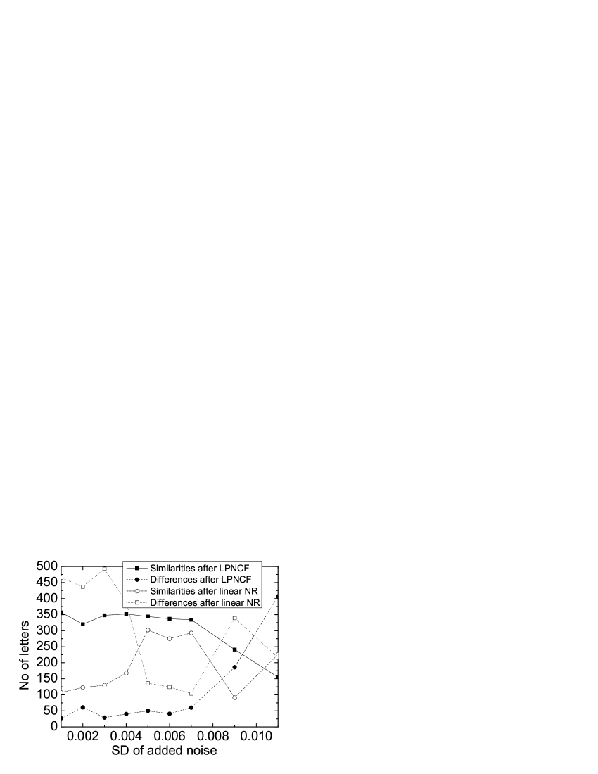
Figure 3: Plot of similarities and differences in letters of the correct text and texts recognized from noisy signals after noise reduction using LPNCF method (solid squares and circles) or texts recognized from noisy signals after optimal linear noise reduction (open squares and circles). Standard deviation of added noise appears at the x-axis.

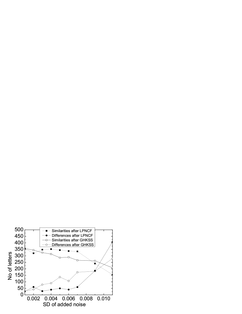
Figure 4: Plot of similarities and differences in letters of the correct text and texts recognized from noise signals after noise reduction using LPNCF method (solid squares and circles) or texts recognized from noisy signals after noise reduction using GHKSS method (open squares and circles). Standard deviation of added noise appears at the x-axis.

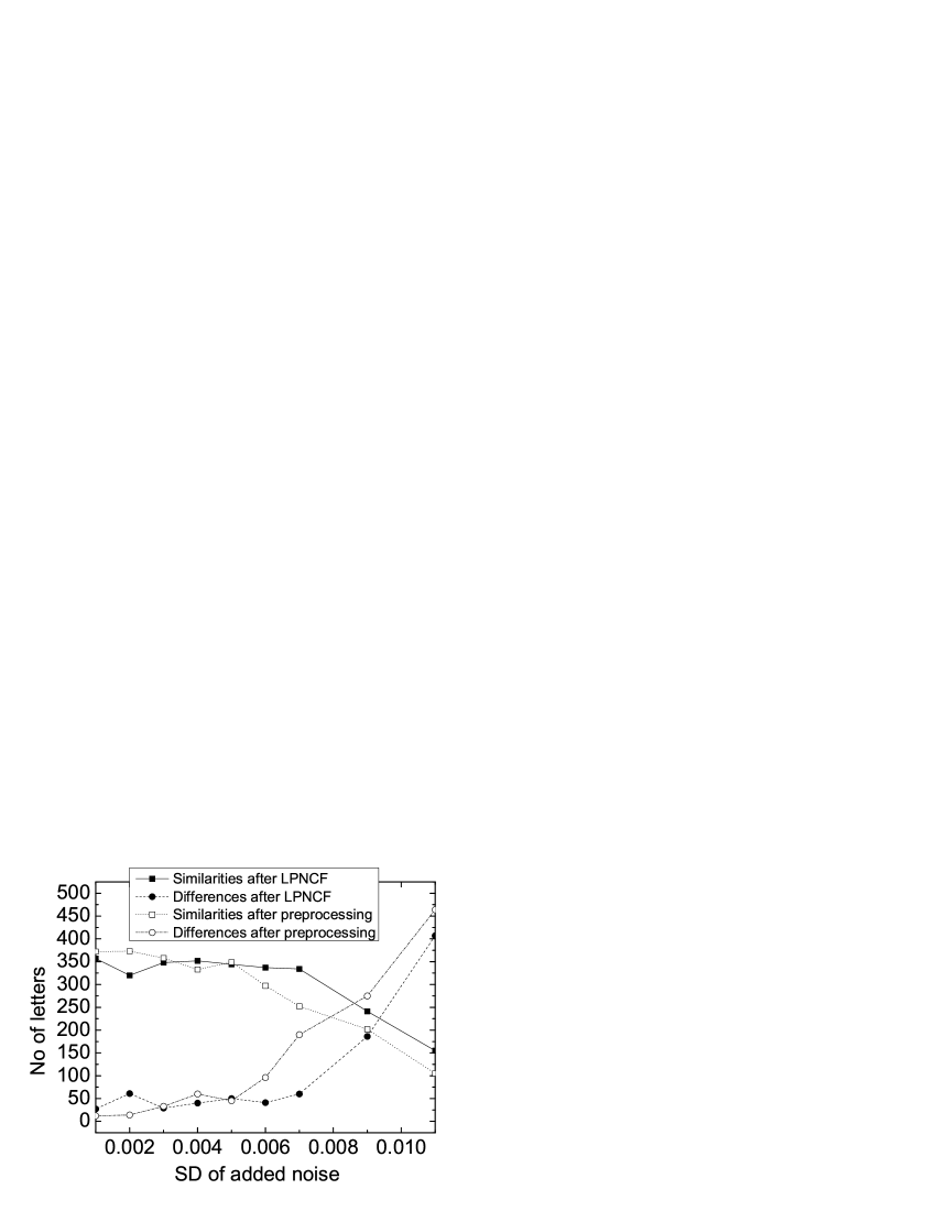
Figure 5: Plot of similarities and differences in letters of the correct text and texts recognized from noisy signals after noise reduction using LPNCF method (solid squares and circles) or texts recognized from noisy signals after preprocessing analysis (open squares and circles). Standard deviation of added noise appears at the x-axis.

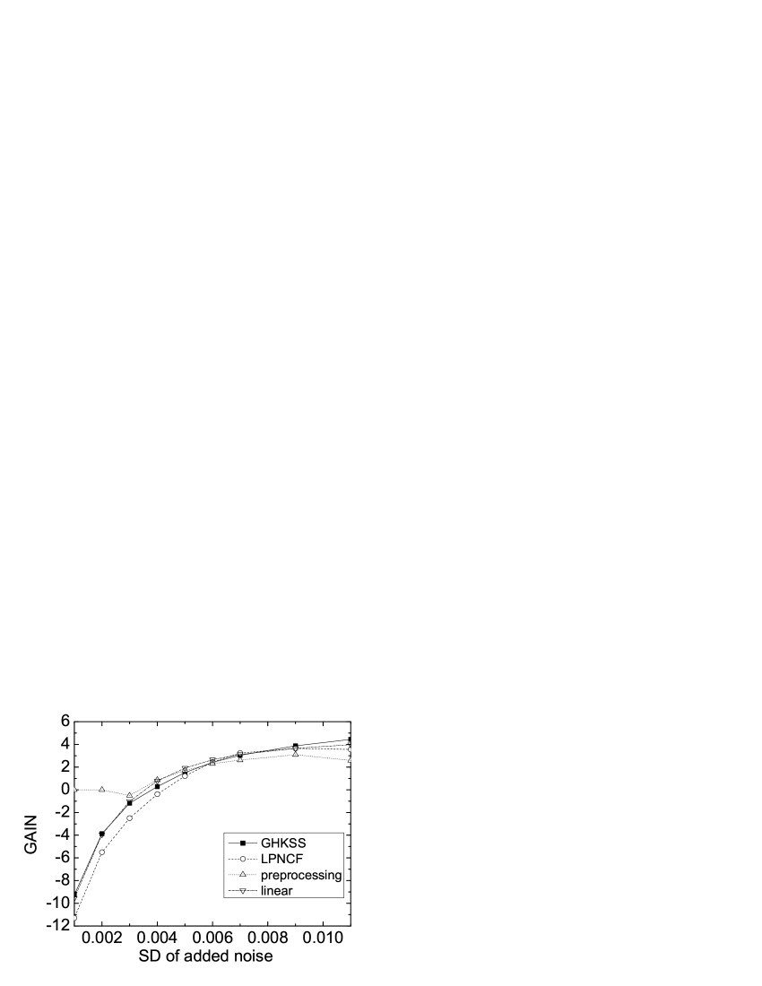
Figure 6: Plot of the gain parameter versus SD of added noise in the signal.

VI acknowledgement

The work has been supported by the Project STOCHDYN by European Science Foundation and by Polish Ministry of Science and Higher Education (Grant 15/ESF/2006/03).

References

- (1) E.J. Kostelich and T. Schreiber, Phys. Rev. E 48(3),1752 (1993).
- (2) T. Schreiber, Phys. Rev. E 48(1),13(4) (1993).
- (3) T. Schreiber, Phys. Rev. E 47(4),2401 (1992).
- (4) J. D. Farmer and J.J. Sidorowich, Physica D 47, 373-392 (1991).
- (5) S.M. Hammel, Phys. Lett. A 148, 421 (1990).
- (6) M.E. Davies, Physica D 79, 174 (1994).
- (7) R. Cawley and G. H. Hsu, Phys. Rev. A 46(6), 3057 (1992).
- (8) T. Sauer, Physica D 58, 193 (1994).
- (9) P. Grassberger, R. Hegger, H. Kantz, C. Schaffrath and T. Schreiber, Chaos 3(2),127 (1993).
- (10) R. Hegger, H. Kantz and L. Matassini, Phys. Rev. Lett. 84, 3197-3200 (2000).
- (11) H. Kantz. R. Hegger, L. Matassini, IEEE Trans. Circuits and Systems I, 48, 1454 (2001).
- (12) K. Urbanowicz and J.A. Hołyst, Acta Phys. Pol B 36(9), 2805 (2005), arXiv:cond-mat/0411324.
- (13) K. Urbanowicz, J.A. Hołyst, T. Stemler and H. Benner, Acta Phys. Pol B 35 (9), 2175 (2004); arXiv:cond-mat/0308554.
- (14) A. Leontitsis, T. Bountis, J. Pagge, CHAOS 14, 1006 (2004).
- (15) W.H. Press, S.A. Teukolsky, W.T. Vetterling, B.P. Flannery, Numerical Recipes in C. The Art of Scientific Computing. Second Edition, (Cambridge University Press, Cambridge, 2002).
- (16) Linguatec web page: http://www.linguatec.de