APPLICATIONS OF PHYSICS
TO FINANCE AND ECONOMICS:
RETURNS, TRADING ACTIVITY AND INCOME

Abstract

Abstract: This dissertation reports work where physics methods are applied to financial and economical problems. Some material in this thesis is based on $3$ published papers SY ; SPY ; income which divide this study into two parts. The first part studies stock market data (chapter 1 to 5). The second part is devoted to personal income in the USA (chapter 6).

We first study the probability distribution of stock returns at mesoscopic time lags (return horizons) ranging from about an hour to about a month. While at shorter microscopic time lags the distribution has power-law tails, for mesoscopic times the bulk of the distribution (more than 99% of the probability) follows an exponential law. The slope of the exponential function is determined by the variance of returns, which increases proportionally to the time lag. At longer times, the exponential law continuously evolves into Gaussian distribution. The exponential-to-Gaussian crossover is well described by the analytical solution of the Heston model with stochastic volatility.

After characterizing the stock returns at mesoscopic time lags, we study the subordination hypothesis with one year of intraday data. We verify that the integrated volatility $V_{t}$ constructed from the number of trades process can be used as a subordinator for a driftless Brownian motion. This subordination will be able to describe $\approx 85\%$ of the stock returns for intraday time lags that start at $\approx 1$ hour but are shorter than one day (upper time limit is restricted by the short data span of one year). We also show that the Heston model can be constructed by subordinating a Brownian motion with the CIR process. Finally, we show that the CIR process describes well enough the empirical $V_{t}$ process, such that the corresponding Heston model is able to describe the log-returns $x_{t}$ process, with approximately the maximum quality that the subordination allows ($80\%-85\%$).

Finally, we study the time evolution of the personal income distribution. We find that the personal income distribution in the USA has a well-defined two-income-class structure. The majority of population (97–99%) belongs to the lower income class characterized by the exponential Boltzmann-Gibbs (“thermal”) distribution, whereas the higher income class (1–3% of population) has a Pareto power-law (“superthermal”) distribution. By analyzing income data for 1983–2001, we show that the “thermal” part is stationary in time, save for a gradual increase of the effective temperature, whereas the “superthermal” tail swells and shrinks following the stock market. We discuss the concept of equilibrium inequality in a society, based on the principle of maximal entropy, and quantitatively show that it applies to the majority of population.

I Introduction

The interest of physicists in interdisciplinary research has been constantly growing and the area of what is today named socio-economical physics is 10 years old Farmer1999 . This new area in physics has started as an exercise in statistical mechanics, where complex behavior arises from relatively simple rules due to the interaction of a large number components. The pioneering work in the modern stream of economical physics was initiated by Mantegna Mantegna and Li Li in the early nineties followed most notably by Mantegna and Stanley Stanley1995 and thereafter by a stream of papers Network that attempt to identify and characterize universal and non-universal features in economical data in general. This statistical mechanical mind frame arises in direct analogy with statistical mechanics of phase transitions, where materials (such as a ferromagnetic and a liquid), that are different in nature, can belong to the same universality class due to their behavior near the critical point (point at which abruptly the phase changes, say from liquid to solid in water, for instance). These universality classes are identified by critical exponents for quantities that diverge at the critical point, for instance the specific heat $C\approx\epsilon^{-\alpha}$, where $\epsilon$ is the reduced temperature and $\alpha$ the critical exponent Stanley . Therefore, the area of economical physics has grown from, and it is still in great part concerned with, “power-law tails” with universal exponents. This constitutes the empirical stream of socio-economical physics, where modelling and characterizing the empirical data with methods and tools borrowed from traditional physical problems is attempted BP ; MS ; R ; V .

Soon after Mantegna and Li initiated the modern empirical stream of economical physics, simulations appeared. Once again, as in the case of empirical work, these were based into fundamental statistical mechanical models such as the Ising model. This literature attempted to construct from simple rules complex behavior that could then mimic the market and explain the price formation mechanism Zhang1997 ; Lane2003 ; Zhang2001 ; Challet2003 ; Challet2005 .

This dissertation belongs to the empirical stream of socio-economical physics. We study here two distinct problems. First, we use daily and intraday stock data to describe the essential nature of the stochastic process of price returns at different time ranges. Second, we use yearly income data to study the time evolution of the distribution of income in the USA.

I.1 Stock returns

The study of stock returns has a long history dating back to Bachalier in $1900$, which was the first to model stock dynamics with a Brownian motion Taqqu . He proposed that the absolute price change $\Delta S_{t}=S_{T}-S_{T-t}$, where $t$ is the return horizon, should follow a Gaussian random walk. The clear drawback of such a hypothesis is that the prices of stocks could become negative. It was apparently Renery Taqqu ; Laurent ; Osborne , who introduced the geometrical Brownian motion for the stock price by assuming that log-returns ($x_{t}=\ln(S_{T})-\ln(S_{T-t})\approx\Delta S_{t}/S_{t}$), and not absolute returns, should follow a Brownian motion. The geometric Brownian motion became popular and accepted as a main stream idea with the work of Osborne Osborne1959 (see also Taqqu for historical notes) and Samuelson (cited in Taqqu ).

It was not until the $1960$’s, that the hypothesis of Gaussian random walks was challenged by Mandelbrot Mandelbrot1963 and Fama Fama1963 ; Fama1965 with studies on daily cotton prices. Since then, Brownian motion has been consistently questioned for a variety of assets. Today asset log-returns that follow Brownian motion for all return horizons $t$ are considered an exception.

In his pioneering work, Mandelbrot introduced, as an alternative model for stock returns, the stable Lévy distribution. This distribution has the drawback that it can present infinite variance. Despite the unwanted mathematical properties that such a process presents, it was not founded into economical reasoning. In $1973$ Clark Clark proposed, as an alternative to Mandelbrot’s model, to use subordination FellerBook to construct the distribution of assets returns. Subordination has a direct financial implication, it can be liked with financial information arrival. Clark suggests that prices react to financial information and that if this financial information is taken into account, the gaussian random walk is recovered. He showed that the information arrival can be captured by volume of trades and that if one takes returns conditional on the volume, these should be Gaussian.

Note that in fact, Mandelbrot and Clark do not contradict themselves, as Clark first implied. Mandelbrot’s Lévy stable distribution can also be constructed by subordination, if one chooses the right subordinator for the Brownian motion. Therefore, the problem is reduced to finding the right subordinator if one accepts the subordination hypothesis.

In physics, the concept of subordination can be found in the construction of non-Shannon entropies, in the limit of the continuous-time random walk, in interface growth models and other statistical mechanical problems Cohen2003 ; FGIS ; Sokolov2001a ; Sokolov2001b ; Sokolov2002 . The mathematical- “physical” idea of subordination is that if the stochastic process is analyzed at the correct reference frame, it will always look like a simple gaussian diffusion. But since we are dealing with stochastic processes, the reference frame is moving randomly as well; just enough for the actual process in observation to be described by Brownian motion. For further mathematical development of subordination, see section V.3.

After Clark, the concept of subordination has been extensively used to construct asset return models LevyBook ; Madan1990 ; NIG1995 ; CGMY . Most recently a series of studies have used high-frequency data to verify Clark’s subordination hypothesis by either assuming that the volume Smith1994 ; Manganelli2000 or the trading activity (number of trades) Ane2000 ; Stanley2000 is responsible for price changes. Strong evidence is found for both; nonetheless number of trades appears better suited, since it has been extensively tested for a large number of companies Stanley2000 .

Contemporary to Clark, a series of empirical studies indicated that the variance ($variance=volatility^{2}$) of stock returns is not constant (see Johnson1987 and references therein). This resulted in models for stock returns such as Engle’s ARCH and Bollerslev’s GARCH that attempted to account for the changing variance in the assets returns by modelling both in a discrete framework Engle2003 . At the same time, models with stochastic volatility were introduced. These models generally assume a mean reverting continuous stochastic differential equation for the volatility Sircar ; Hull1987 ; Heston ; options . Notice that stochastic volatility models, GARCH and subordination, are not entirely orthogonal to each other. Stochastic volatility models can also be constructed by subordination CGMYSA (see also section V.3) or as limits of discrete GARCH type models Heston2003 .

In $1993$ Heston Heston introduced an exactly solvable stochastic volatility model that is also a limit process for the GARCH(1,1) model Heston2003 . The Heston model become widely used for option pricing and in the study of asset returns. We use a modified version of the Heston model as developed in Ref. DY to describe the general shape of probability density distribution (PDF) for the log-returns and the time evolution of such PDF.

I.2 Outline of the dissertation

The outline of this thesis is as follows. In chapter II, we introduce the Heston model for stock returns as developed in Refs. SPY ; DY . We summarize the procedure for finding the closed form solution of the probability distribution for the log-returns, starting from the correlated stochastic differential equations as given in Ref. DY . We also introduce subordination and show how to construct the Heston model using a Cox-Ingersoll-Ross (CIR) subordinator CIR .

In chapter III, we present the data we use in this thesis. We show the typical features of the stock data and how we constructed such data.

In chapter IV, we study the time evolution of the empirical distribution function (EDF) for the stock returns at mesoscopic time lags $t$ ($1\,hour<t<20\,days$). We show that in the short-time limit $t<<1/\gamma$, the EDF progressively tends to the double exponential distribution and for the long-time limit $t>>1/\gamma$, the EDFs progressively tends towards a Gaussian, where $1/\gamma$ is the characteristic time for such limits. Furthermore, we show that the Heston model introduced in chapter II presents these fundamental features.

In chapter V, we study the hypothesis of subordination. We first start by pointing out the effect of the discrete nature of absolute price changes in the log-returns. Thereafter, we verify the subordination hypothesis using both tick-by-tick data (this data records all trades in a given day, see chapter III) as well as $5$ minutes log-returns and number of trades (ticks) data. We find that if we use the integrated variance ($V_{t}$), which is proportional to the number of trades ($N_{t}$), as our subordinator, we are able to explain approximately the central $85\%$ of the probability distribution for the log-returns $x_{t}$ between $1$ hour and $1$ day. Finally, we show the quality of modelling the subordinator $V_{t}$ with the CIR process introduced in section V.3 and discuss the implication of such model for the log-returns $x_{t}$.

The last chapter of this thesis presents work on the time evolution of the distribution of income. We show the evolution of the distribution of personal income in the United States from $1983$ to $2001$. We show that the bulk of the distribution (excluding very small income and very large income), is described by the Exponential distribution with average income changing from year to year in approximately the same rate as inflation. We conclude that the inflation-discounted income of the majority of the population is approximately the same throughout time and therefore well approximated by a system in thermal equilibrium. We also show that the top $3\%$ earners have income that changes over time even when inflation is accounted for. This chapter is self contained and does not require any other part of the thesis to be read.

II Heston model for asset returns

The Heston model was introduced by Heston Heston and belongs to the class of stochastic volatility models, which have received a great deal of attention in the financial literature specially in connection with option pricing Sircar .

Empirical verification of the Heston model was done for both stocks SY ; SPY ; DY ; Pan ; Vicente and options Hull1987 ; Bakshi ; Duffie ; options , and good agreement with the data has been found in these studies. The version of the Heston model for stock returns used in SY ; SPY ; DY , as well as in this thesis, was modified from the original solution by Heston and has evolved into a different formula with $3$ parameters. One parameter for the variance ($\theta$), one parameter representing the characteristic relaxation time to the Gaussian distribution ($1/\gamma$) and another that gives the general shape of the curve ($\alpha$).

The outline of this chapter is as follows. First, we present the modified Heston model used in this work by showing its evolution from solving the related stochastic differential equations (SDE). Thereafter, we introduce subordination and we show the development of the modified Heston model through subordination.

II.1 Heston model-SDE and symmetrization

The formal way of presenting the Heston model is given by two stochastic differential equations (SDE), one for the stock price $S_{t}$ and another for the variance $v_{t}$.

$$dS_{t}=\mu S_{t}\,dt+\sigma_{t}S_{t}\,dW_{t}^{(1)},$$ (1)

$$dv_{t}=-\gamma(v_{t}-\theta)\,dt+\kappa\sqrt{v_{t}}\,dW_{t}^{(2)},$$ (2)

where the subscript $t$ indicates time dependence, $\mu$ is the drift parameter, $W_{t}^{(1)}$ and $W_{t}^{(2)}$ are standard random Wiener processes, $\sigma_{t}$ is the time-dependent volatility and $v_{t}=\sigma_{t}^{2}$ is the variance. In general, the Wiener process in (2) may be correlated with the Wiener process in (1):

$$dW_{t}^{(2)}=\rho\,dW_{t}^{(1)}+\sqrt{1-\rho^{2}}\,dZ_{t},$$ (3)

where $Z_{t}$ is a Wiener process independent of $W_{t}^{(1)}$, and $\rho\in[-1,1]$ is the correlation coefficient. Note that (1) and (2) are well known in finance. These represent, respectively, the log-normal geometric Brownian motion stock process introduced by Renery, Osborne and Samuelson Taqqu (used by Black-Melton-Scholes (BMS) BS ; Merton for option pricing. See Ref. BSinPhysics for a practical application of BMS to physics) and the Cox-Ingersoll-Ross (CIR) mean-reverting SDE first introduced for interest rate models CIR ; Shreve .

In order to solve (1) and (2) together with (3), we first change variables from stock price $S_{t}$ to mean removed (demean) log-return $x_{t}=ln(S_{t}/S_{0})-\mu t$ (4). All further results and solutions are constructed for the demean log-return $x_{t}$, which we will simply refer to as log-return or return:

$$dx_{t}=-\frac{v_{t}}{2}\,dt+\sqrt{v_{t}}\,dW_{t}^{(1)}.$$ (4)

After performing the change of variables from price to return, we solve the Fokker-Planck equation (II.1) Gardiner implied by SDEs (2) and (4), for the transition probability $P_{t}(x,v\,|\,v_{i})$ to find the return $x$ and the volatility $v$ at time $t$ given the initial demean log-return $x=0$ and variance $v_{i}$ at $t=0$. For simplicity, we drop the explicit time dependence notation for the returns $x_{t}$ and call them $x$.

$$\frac{\partial}{\partial t}P = \gamma\frac{\partial}{\partial v}\left[(v-\theta)P\right]+\frac{1}{2}\frac{\partial}{\partial x}(vP)$$

$${}+\rho\kappa\frac{\partial^{2}}{\partial x\,\partial v}(vP)+\frac{1}{2}\frac{\partial^{2}}{\partial x^{2}}(vP)+\frac{\kappa^{2}}{2}\frac{\partial^{2}}{\partial v^{2}}(vP).$$

The general analytical solution of (II.1) for $P_{t}(x,v\,|\,v_{i})$ with initial condition $P_{t=0}(x,v|\,v_{i})=\delta(x)\delta(v-v_{i})$ can be found by taking a Fourier transform $x->p_{x}$ and a Laplace transform $v->p_{v}$ (see DY for details),

$$P_{t}(x\,|\,v_{i})=\int\limits_{0}^{+\infty}\!\!dv\,P_{t}(x,v\,|\,v_{i})=\int\frac{dp_{x}}{2\pi}e^{ip_{x}x}\widetilde{P}_{t,p_{x}}(0\,|\,v_{i}),$$ (6)

where the hidden variable $v$ is integrated out, so $p_{v}=0$. Therefore we have

$$P_{t}(x\,|\,v_{i})=\int_{-\infty}^{+\infty}\frac{dp_{x}}{2\pi}\,e^{ip_{x}x-v_{i}\frac{p_{x}^{2}-ip_{x}}{\Gamma+\Omega\coth{(\Omega t/2)}}}$$

$$\times\,e^{-\frac{2\gamma\theta}{\kappa^{2}}\ln\left(\cosh\frac{\Omega t}{2}+\frac{\Gamma}{\Omega}\sinh\frac{\Omega t}{2}\right)+\frac{\gamma\Gamma\theta t}{\kappa^{2}}}.$$ (7)

where

$$\Gamma=\gamma+i\rho\kappa p_{x}$$ (8)

and

$$\Omega=\sqrt{\Gamma^{2}+\kappa^{2}(p_{x}^{2}-ip_{x})}.$$ (9)

The marginal probability density $P_{t}(x\,|\,v_{i})$ could then be compared to empirical stock returns directly. Nevertheless, $v_{i}$ has to be treated as an extra parameter. In order to avoid this, we assume that $v_{i}$ has the stationary distribution of the CIR stochastic differential equation (2), $\Pi_{\ast}(v)$,

$$\Pi_{\ast}(v)=\frac{\alpha^{\alpha}}{\Gamma(\alpha)}\,\frac{v^{\alpha-1}}{\theta^{\alpha}}\,e^{-\alpha v/\theta},\qquad\alpha=\frac{2\gamma\theta}{\kappa^{2}}.$$ (10)

Using equation (10) we arrive at the probability distribution of the demean log-returns $P_{t}(x)$,

$$P_{t}(x)=\int_{0}^{\infty}\!\!dv_{i}\,\Pi_{\ast}(v_{i})\,P_{t}(x\,|\,v_{i})$$ (11)

where the final solution is

$$P_{t}(x)=\frac{1}{2\pi}\int_{-\infty}^{+\infty}\!\!dp_{x}\,e^{ip_{x}x+F_{t}(p_{x})}$$ (12)

with

$$F_{t}(p_{x})=\frac{\gamma\theta}{\kappa^{2}}\,\Gamma t$$ (13)

$${}-\frac{2\gamma\theta}{\kappa^{2}}\ln\left[\cosh\frac{\Omega t}{2}+\frac{\Omega^{2}-\Gamma^{2}+2\gamma\Gamma}{2\gamma\Omega}\sinh\frac{\Omega t}{2}\right]$$

where as before

$$\Gamma=\gamma+i\rho\kappa p_{x}$$ (14)

and

$$\Omega=\sqrt{\Gamma^{2}+\kappa^{2}(p_{x}^{2}-ip_{x})}.$$ (15)

The operation of removing the initial volatility dependence of the marginal probability density $P_{t}(x\,|\,v_{i})$ using equation (11) was first introduced in Ref. DY . This removes an additional degree of freedom and therefore simplifies the final marginal probability density.

In order to further simplify the original Heston model, we assume that equations (1) and (2) are uncorrelated. That amounts in taking $\rho=0$ in expression (13). This approximation was shown to be acceptable for some companies and indexes in the US market SY ; SPY ; DY but might not be good for different markets Vicente or for option pricing Sircar ; Heston .

In order to arrive at the probability density function used in this work, we need to further simplify the equation for $P_{t}(x,\rho=0)$ (12) into a zero skew symmetrical function.

We replace in (12) $p_{x}\to p_{x}+i/2$ and $\rho=0$ to find

$$P_{t}(x)=e^{-x/2}\int_{-\infty}^{+\infty}\frac{dp_{x}}{2\pi}\,e^{ip_{x}x+F_{t}(p_{x})},$$ (16)

where $\alpha=2\gamma\theta/\kappa^{2}$,

$$F_{t}(p_{x})=\frac{\alpha\gamma t}{2}-\alpha\ln\left[\cosh\frac{\Omega t}{2}+\frac{\Omega^{2}+\gamma^{2}}{2\gamma\Omega}\sinh\frac{\Omega t}{2}\right],$$ (17)

and

$$\Omega=\sqrt{\gamma^{2}+\kappa^{2}(p_{x}^{2}+1/4)}\approx\gamma\sqrt{1+p_{x}^{2}(\kappa^{2}/\gamma^{2})}.$$ (18)

Finally, we drop the $e^{-x/2}$ term in (16). Notice that both taking $e^{-x/2}\approx 1$ and $p_{x}^{2}+1/4\approx p_{x}^{2}$ are needed to produce a new characteristic function $e^{F_{t}(p_{x})}$ that correctly goes to unity when $p_{x}=0$. The final functional form for $P_{t}(x)$ is

$$P_{t}(x)=\int\limits_{-\infty}^{+\infty}\frac{dp_{x}}{2\pi}\,e^{ip_{x}x+F_{\tilde{t}}(p_{x})},$$ (19)

$$F_{\tilde{t}}(p_{x})=\frac{\alpha\tilde{t}}{2}-\alpha\ln\left[\cosh\frac{\Omega\tilde{t}}{2}+\frac{\Omega^{2}+1}{2\Omega}\sinh\frac{\Omega\tilde{t}}{2}\right],$$ (20)

$$\tilde{t}=\gamma t,\quad\alpha=2\gamma\theta/\kappa^{2},$$

$$\Omega=\sqrt{1+(p_{x}\kappa/\gamma)^{2}},\quad\sigma_{t}^{2}\equiv\langle x^{2}\rangle=\theta t.$$ (21)

We have expressed the original Heston model for the probability density of log-returns $x$, in a highly symmetrical form with three parameters, $\theta$, $\alpha$ and $\gamma$. The parameter $\theta$ can be found by calculating the variance of demean log-returns $\sigma_{t}^{2}\equiv\langle x_{t}^{2}\rangle=\theta t$ (21) of $P_{t}(x)$ (19). The remaining two parameters, $\alpha$ and $\gamma$, are responsible for the general shape of the curve and the relaxation rate of $P_{t}(x)$ to a Gaussian distribution SPY ; DY . The parameter $\alpha$ is also responsible to define the analyticity at zero return. If $\alpha=1$, value used in this thesis, the short-time-limit is a double exponential distribution (see next subsection). This distribution is not analytical at zero but becomes when time progresses. For $\alpha>1$ the distribution is always analytical with a center that is Gaussian and when $\alpha<1$ the distribution starts non-analytic at zero (going to zero as a power-law with exponent $2\alpha-1$ DY ) and then evolves into a analytic distribution with Gaussian center.

Notice that the average for the log-returns $x$ from equation (19) is $\langle x\rangle=0$. This average is not consistent with SDE (4), but with the simplified $dx_{t}=\sqrt{v_{t}}dW_{t}^{(1)}$, where the drift term $v_{t}/2$ is set to zero. Therefore, $x$ in equation (19) does only approximately represent demean log-returns $x=ln(S_{t}/S_{0})-\mu t$. This difference arises because we took $e^{-x/2}\approx 1$ and $p_{x}^{2}+1/4\approx p_{x}^{2}$ in equation (17) in order to derive equation (20).

The log-returns $x$ in equation (19) can be exactly given by $x=ln(S_{t}/S_{0})-\mu t-\omega(t)$, where the extra term, $\omega(t)$, removes the non zero average of $x=ln(S_{t}/S_{0})-\mu t$.

The extra term $\omega(t)$ arises because the average of the stock price at time $t$ needs to be given by $\mu$ only. Hence

$$\langle S_{t}\rangle=S_{0}e^{\mu t}\langle e^{Y_{t}}\rangle,\,\langle e^{Y_{t}}\rangle\equiv 1,$$ (22)

where $Y_{t}$ is the stochastic process

$$S_{t}=S_{0}\frac{e^{\mu t+X_{t}}}{<e^{X_{t}}>}=S_{0}e^{\mu t-ln(<e^{X_{t}}>)+X_{t}}$$

$$\Rightarrow\omega(t)=-ln(<e^{X_{t}}>)$$

$$x_{t}=ln(S_{t})-ln(S_{0})-\mu t=X_{t}+\omega(t)$$

$$\Rightarrow Y_{t}=X_{t}+\omega(t).$$ (23)

Empirically, the correction represented by $\omega(t)$ or by working with equation (16) instead of equation (19) is small, and it can be safely neglected. We choose to work with $x=ln(S_{t}/S_{0})-\mu t-\omega(t)$, and we call $x$ in (19) the log-return.

II.1.1 Short and long time limits of the Heston model

The short time lag limit of the modified Heston model (19) can be found by assuming $\Omega t\ll 2$ in expression (II.1). We also take $\rho=0$ and $ip_{x}\rightarrow 0$, since we interested in the short-time-limit of the symmetric modified Heston model of equation (19). When taking the limit $\Omega t\ll 2$ in (II.1), the resulting PDF is the Fourier inverse of the characteristic function of a Gaussian with random variance $v_{i}$ and zero drift. Since $v_{i}$ is a Gamma random variable with distribution (10), the final characteristic function for the short-time-limit distribution of the modified Heston model is

$$\tilde{P}_{t}(p_{x})=\int_{0}^{\infty}dv_{i}e^{\frac{-v_{i}p_{x}t}{2}}\Pi_{*}(v_{i})=(1+\frac{\theta tp_{x}^{2}}{2\alpha})^{-\alpha}.$$ (24)

The probability distribution can be found analytically DY as

$$P_{t}(x)=\frac{2^{1-\alpha}}{\Gamma(\alpha)}\,\sqrt{\frac{\alpha}{\pi\theta t}}\,y^{\alpha-1/2}K_{\alpha-1/2}(y),$$ (25)

where $K$ is the modified Bessel function and

$$y=\sqrt{\frac{2\alpha x^{2}}{\theta t}}.$$ (26)

For $\alpha=1$, we recover the Laplace (symmetrical double exponential) distribution

$$P_{t}(x)=\frac{e^{-y}}{\sqrt{2\theta t}},\,y=\sqrt{\frac{2\alpha x^{2}}{\theta t}}.$$ (27)

Notice that the short time limit is not a Gaussian with variance $v_{i}$, only because of the assumed randomization of $v_{i}$ (24). Therefore, this randomization has substantial effect in the limiting distributions, which can be checked empirically SPY (empirical results will be presented in chapter IV).

The long time lag $t$ limit for the modified Heston model can be found by taking the limit $\Omega t\gg 2$ in the characteristic function (20). The resulting characteristic function is

$$\tilde{P}_{t}(p_{x})=\langle e^{ip_{x}x}\rangle=e^{\frac{\alpha\gamma t}{2}\left(1-\sqrt{1+x_{0}^{2}p_{x}^{2}}\right)},\,x_{0}=\kappa^{2}/\gamma^{2}.$$ (28)

The characteristic function in equation (28) is the characteristic function for the zero skew Normal Inverse Gaussian (NIG) model. NIG was first introduced by Barndorff-Nielsen to describe the distribution of sand particles sizes BN1977 and was subsequently used in other physical problems such as turbulence BN1979 . In $1995$, Barndorff-Nielsen also introduced NIG for stock returns NIG1995 . NIG can also be obtained as a limit of the Generalized Hyperbolic distribution LevyBook ; Eberlein2002 , as well as by subordinating a Brownian motion to the inverse gaussian distribution LevyBook (next section will introduce the idea of subordination).

NIG is part of the wide class of Lévy pure jump models LevyBook , and the fact that it is recovered as a limit of the simplified Heston stochastic volatility model (19), is another consequence of the randomization of $v_{i}$. Notice that if we take the long time limit before the randomization of $v_{i}$ in the full Heston model given in Eq. (II.1), we will not find NIG as the long time limit.

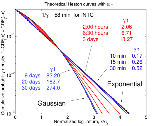
The central limit theorem can be invoked for NIG and therefore for Heston BP ; FellerBook ; NIG1995 ; DY . That is, as time progresses, the distribution $P_{t}(x)$ of returns $x$ will become increasingly Gaussian. The characteristic time scale for the central limit theorem to act is $t_{0}=2/(\alpha\gamma)$. For $t\gg t_{0}$ the probability distribution is essentially Normal with mean zero and variance $\theta t$.

Notice that for long time lags $t$, there are two characteristic time limits. Heston tends to NIG for times $t\gg 1/\gamma$ and then NIG tends to a Normal distribution for times $t\gg 1/\alpha\gamma$. If $\alpha\geq 1$, NIG and Heston regimes can not be effectively distinguished. It is only in the case $\alpha<1$, that there will be a distinguished NIG regime.

In summary, the most important limits for $P_{t}(x)$ that we use in this study are: Exponential (if $\alpha=1$) at short time lags and Gaussian at long time lags,

$$P_{t}(x)\propto\left\{\begin{array}[]{ll}\exp(-|x|\sqrt{2/\theta t}),&\quad\tilde{t}=\gamma t\ll 1,\\ \exp(-x^{2}/2\theta t),&\quad\tilde{t}=\gamma t\gg 1.\end{array}\right.$$ (29)

II.2 Heston model and subordination

Subordination is a form of randomization in which one constructs a new probability distribution, by assuming one or more parameters of the original probability distribution to be random FellerBook ,

$$P_{New}(y,z)=\int_{-\infty}^{\infty}d\theta P(y,\theta)Q(\theta,z).$$ (30)

In the case of subordination, a Markov process $Y(N)$ is randomized by introducing a non-negative process $N(t)$, called a randomized operational time. The resulting process $Y(N(t))$ does not need to be Markovian in general FellerBook . We restrict ourselves to subordination of a Brownian motion with drift $\theta$ and standard deviation $\sigma$ (31). We also assume in what follows, that $t$ is time lag in usual units of time, unless otherwise indicated. The probability density $P_{t}(y)$ for the time changed Brownian motion $Y(N)$ can be written

$$P_{t}(y)=\int_{0}^{\infty}dN\frac{1}{\sqrt{2\pi\sigma^{2}N}}e^{\frac{-(y-\theta N)^{2}}{2\sigma^{2}N}}P_{t}(N).$$ (31)

The moments of a Brownian subordinated process are related to the moments of the subordinator. If we use $P_{t}(y)$ in (31), the first $4$ moments can be calculated as

$$\langle y\rangle=\theta\langle N\rangle_{N}$$ (32)

$$\langle(y-\langle y\rangle)^{2}\rangle=\sigma^{2}\langle N\rangle_{N}+\theta^{2}\langle(N-\langle N\rangle_{N})^{2}\rangle_{N}$$ (33)

$$\langle(y-\langle y\rangle)^{3}\rangle=3\sigma^{2}\theta\langle(N-\langle N\rangle_{N})^{2}\rangle_{N}+\theta^{3}\langle(N-\langle N\rangle_{N})^{3}\rangle_{N}$$ (34)

$$\langle(y-\langle y\rangle)^{4}\rangle=3\sigma^{4}(\langle(N-\langle N\rangle_{N})^{2}\rangle_{N}+\langle N\rangle_{N}^{2})+$$

$$6\theta^{2}\sigma^{2}(\langle(N-\langle N\rangle_{N})^{3}\rangle_{N}+$$

$$\langle N\rangle_{N}\langle(N-\langle N\rangle_{N})^{2}\rangle_{N})+\theta^{4}\langle(N-\langle N\rangle_{N})^{4}\rangle_{N},$$ (35)

where $\langle\rangle$ refers to taking the expected value and $\langle\rangle_{N}$ refers to taking the expected value with respect to $N$. The time $t$ dependence of the moments of $Y$ are given by the moments of the randomized operational time $N$. Furthermore, even though the subordinator has odd moments, odd moments in the resulting process $Y$ are only different from zero, if the Gaussian in equation (31) has a drift $\theta\neq 0$. For the present work, we assume that the odd moments are all zero since the empirical probability distribution of log-returns are quite well described by zero skew probability distributions and because we work with mean zero returns SPY . By assuming zero odd moments probability distribution, we simplify the even moments. The second and fourth moments for $Y$ depend only on the first and second moments of the subordinator $N$ (33,35).

In the case of the modified Heston model (19), the subordination takes the following terms. We assume that the log-returns $x$ follow a Brownian motion with zero drift and variance $V_{t}$. The variance $V_{t}$ is our “random operational time”, since it changes randomly. We will show in chapter V that the variance $V_{t}$ can be estimated (at least partially) using the number of trades $N_{t}$ that occur in a the time interval $t$. The variance $V_{t}$ is then a constant times $N_{t}$, $V_{t}=\sigma^{2}N_{t}$.

The variance $V_{t}$ is given by $V_{t}=\int_{0}^{t}ds\,v_{s}$, where the instantaneous variance $v_{t}$ appearing in the SDE (2) is integrated in the interval $0\rightarrow t$. For this reason, $V_{t}$ is also know as integrated variance. The Laplace transform for the conditional probability density $P_{t}(V_{t}|\,v_{i})$ is analytically known LevyBook ; CIR . Therefore, subordination becomes a useful tool to construct asset models with stochastic variance having the CIR process as a subordinator CGMYSA .

The Laplace transform of the subordinator of the modified Heston model (20) can be read off immediately,

$$\tilde{P}(p_{x})=\langle e^{ip_{x}x}\rangle\Rightarrow\tilde{P}(p_{x})=\int_{0}^{\infty}dV_{t}e^{-\frac{p_{x}^{2}V_{t}}{2}}P(V_{t})$$ (36)

where the integral with respect to $V_{t}$ defines a Laplace transform of the probability density $P(V_{t})$, for which the Laplace conjugated variable is calculated at $p_{x}^{2}/2$. Therefore we arrive at

$$P_{t}(V_{t})=\int\limits_{0}^{+\infty}dp_{V_{t}}\,e^{p_{V_{t}}x+F_{\tilde{t}}(p_{V_{t}})},$$ (37)

$$F_{\tilde{t}}(p_{V_{t}})=\frac{\alpha\tilde{t}}{2}-\alpha\ln\left[\cosh\frac{\Omega\tilde{t}}{2}+\frac{\Omega^{2}+1}{2\Omega}\sinh\frac{\Omega\tilde{t}}{2}\right],$$ (38)

$$\tilde{t}=\gamma t,\quad\alpha=2\gamma\theta/\kappa^{2},\quad\Omega=\sqrt{1+2(\kappa/\gamma)^{2}p_{V_{t}}}.$$ (39)

The only difference between the characteristic exponent (38) and the characteristic exponent for the Heston model (20) is in $\Omega$, where $p_{V_{t}}$ replaces $p_{x}^{2}/2$ as the Laplace variable for $V_{t}$.

The first and second moments for the integrated CIR process (38) are

$$\langle V_{t}\rangle=\theta t$$ (40)

$$\langle(V_{t}-\langle V_{t}\rangle)^{2}\rangle=\frac{2\theta^{2}}{\alpha\gamma^{2}}(e^{-\gamma t}-1+\gamma t).$$ (41)

The time dependence of the variance (41) shows that the CIR process is not independent and identically distributed (IID). That is expected since we have a mean reverting SDE (2) for the instantaneous variance $v_{t}$ with exponential relaxation to the mean Gardiner ; CIR ; Shreve .

We have shown that subordinating a zero drift gaussian to the integrated $V_{t}$, given by equation (37) is equivalent to solving for the transition probability densities for the uncorrelated ($\rho=0$ in equation (3)) system of SDEs $dx_{t}=\sqrt{v_{t}}dW_{t}^{(1)}$ and $dv_{t}=-\gamma(v_{t}-\theta)dt+\kappa\sqrt{v_{t}}dW_{t}^{(2)}$(2). However, it is not clear how to use subordination in order to produce a stochastic process that is equivalent to the correlated ($\rho\neq 0$) system of SDEs CGMYSA .

III General characteristics of the data and methods

We use 2 databases for this study. Daily closing prices are downloaded from Yahoo Yahoo and intraday data is constructed using the TAQ database from the NYSE TAQ . The TAQ database records every transaction that occurred in the market (tick-by-tick data), where the average number of transactions in a day for a highly traded stock, such as Intel, is $20000$ (from 1993 to 2001). That is equivalent, in terms of data quantity, to approximately $77$ years of daily data.

Our data has the time that the transaction occurred, the price the transaction was realized and the volume of the transaction (number of shares that exchanged hands). The TAQ database does not account for splits or dividends whereas Yahoo gives the prices corrected for splits and dividends. However we do need to correct for splits and dividends because the TAQ database is used only when constructing intraday returns. The splits and dividends are realized overnight and therefore will not show up if we calculate intraday returns.

After downloading the TAQ data, we remove any trade that is recorded as an error and also restrict the data to trades that took place inside the conventional $6.5$ hours trading day from $9\colon 30$ AM to $4\colon 00$ PM. Any trade that happen before $9\colon 30$ AM and after $4\colon 00$ PM is ignored. We choose to restrict to business hours because we want our data set to agree with Yahoo daily data in the limit of one day that is defined from the open bell ($9\colon 30$ AM) to close bell ($4\colon 00$ PM).

Figure 1: Intraday stock price and number of trades constructed from the TAQ database at each $5$ minute interval from Thursday, 2nd of January 1997 to Thursday 9th of January 1997 for Intel (upper panel). Volume of trades during each day is shown in the lower panel. Days are separated by an effective overnight time interval that is constructed from the data, such that the open-to-close variance and the close-to-close variance of the log-returns follow the same $\propto t$ line (see Fig. 5).

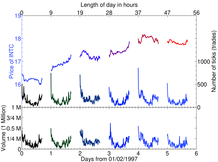
We define as the daily open price, the price of the first trade that happened after or at $9\colon 30$ AM. We also define the daily close price, the price of the trade that happened right before or at $4\colon 00$ PM. A typical time series for intraday prices, number of trades and volumes for $1$ particular week is shown in Fig. 1.

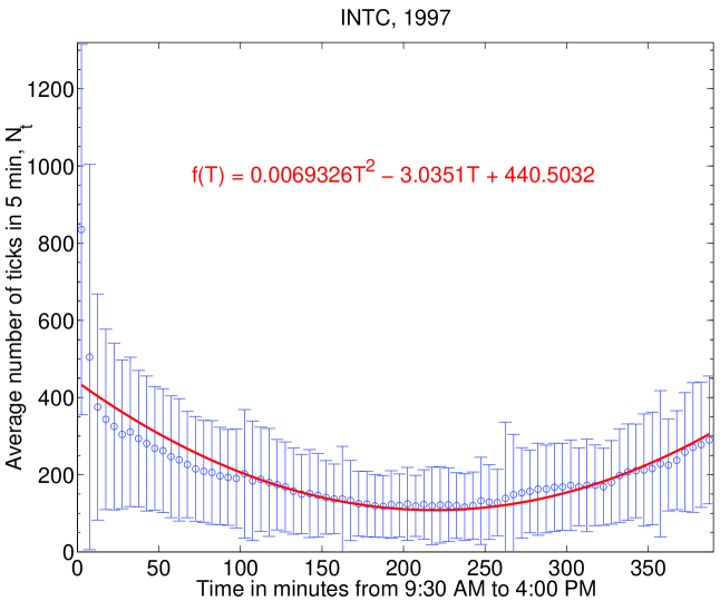
Notice that the intraday volume and trading activity (number of trades) can be well described by a parabola (Fig. 3). This typical intraday pattern Osborne1962 ; Ord1985 has also been found for high-frequency volatility proxies, such as the root mean square return for all ticks that happen in a certain interval of time StanleyVol1999 ; Engle2000 ; Bollerslev1996 ; Bollerslev2001 ; Granger1996a ; Granger1996b . The statistics for such a pattern for the number of trades of Intel in the year $1997$ is shown in Fig. 3. Notice that the probability density for different parts of the day will clearly have different widths and averages. Therefore, mixing all parts of the day will result in a wider probability density for number of trades and other intraday quantities Ord1985 . We do not study the consequences of such a mixture, we only are careful to work with intraday time lags that divide equally all day SPY . In such a way, all parts of the daily trend are equally represented. Since we are working with prices quoted at every $5$ minutes (Five minutes close prices) and the day from open to close has only $78$ such intervals, we work with returns that are $t=5,10,15,30,65,130,195,390$ minutes long.

Figure 2: Cumulative number of trades and return from $1993$ to $2001$ for Intel. The increase of the cumulative number of trades indicate that the parameters describing the stock are changing.

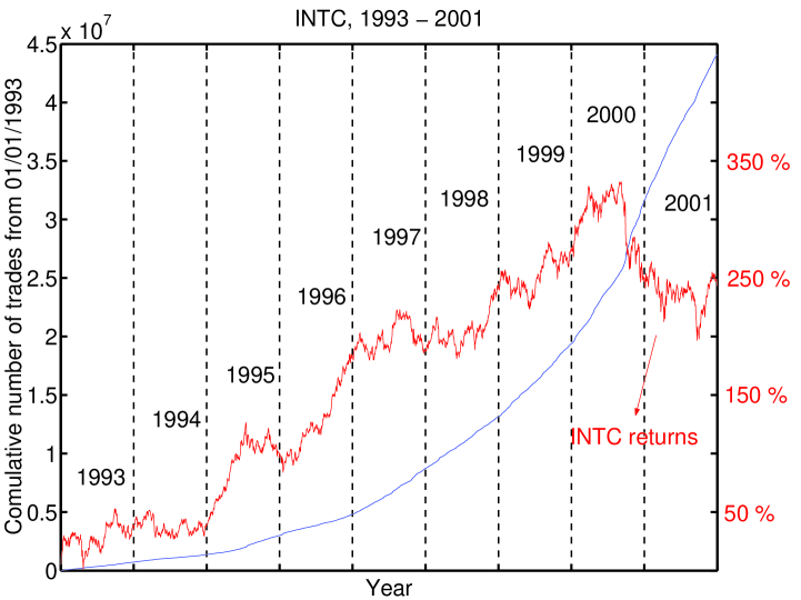
Another important characteristic of daily and intraday data is shown in Fig. 2. The cumulative number of trades from $1993$ to $2001$ ($\sum_{i=01/01/1993}^{i=12/31/2001}N_{i}$) increase almost exponentially. The behavior of the commutative number of trades shows that the average number of trades change from year to year. The same type of behavior is found for the square of the demean log-returns (the variance of the returns). Therefore, the probability density for the returns, volume and number of trades is only approximately stationary throughout the years. When studying returns (chapter IV), we assume the data as stationary, and we take data from $1993$ to $1999$. When studying subordination using the number of trades (chapter V), we reduce the non-stationary effect of the data by working with one year of data.

Figure 3: Average number of trades (ticks) in a given period of the day. The error bars represent the volatility. The red solid line gives the best fit parabola to the average number of trades. Same type of pattern is found for absolute returns StanleyVol1999 and volume.

In order to study intraday returns, we construct from the tick-by-tick data, $5$ minutes close prices. The $5$ minute close price is defined in analogy with the day close price. The 5 minutes volume ( or number of trades (ticks)) is the sum of all traded volume ( or number of trades (ticks)) in a $5$ minutes interval.

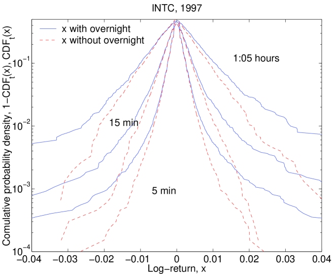
When constructing intraday returns time series, we do not include nights or weekends. Effectively our largest intraday return is from open to close (time lag of 390 min = 6.5 hours). A common procedure, not adopted here, is to assume the open of the next day as the close of the present day Stanley1999a ; Stanley1999b . This will include returns that are effectively overnight, where no trades are present. The result of such practice is illustrated in Fig. 4. Clearly, the tails of the distribution of returns including overnight time lags are considerably enhanced, if compared with the distribution of intraday returns that do not include overnight time lags.

Figure 4: Cumulative density function for the positive and negative log-returns of Intel. Log-returns constructed including overnight time lags (solid lines) show higher probability of large returns than log-returns that do not include overnight time lags (dashed lines). We choose not to include overnight time lags in our intraday return time series.

When working with high-frequency (intraday) data recording errors are inevitable. In order to remove errors in the tick-by-tick data as well as our $5$ minutes close time series, created from the tick-by-tick data, we use Yahoo database as our benchmark. We assume that the daily Yahoo database does not have errors. Our filtering technique consists of two parts. First, we calculate the log-return between the maximum and minimum price of a given day for the Yahoo data ($r_{HL}$). We then calculate the log-return ($r_{5min}=ln(S_{T})-ln(S_{T-5min})$) for the $5$ minutes price data in the same day and compare to $r_{HL}$. We replace any log-return $|r_{t}|>r_{HL}$ with the return immediately preceding it. We also replace the number of trades and volume of the “corrupted” 5 minute interval by the immediately preceding ones. The second filtering procedure consists of requiring that the largest and smallest 5 minutes log-return ($r_{5min}$) in a given day, be between the maximum and the minimum of all the time series formed by the yahoo open to close return data ($min(r_{OC})<r_{5min}<max(r_{OC})$). Once again, if the condition $min(r_{OC})<r_{5min}<max(r_{OC})$ is not satisfied, we replace the “corrupted” log-return, volume and number of trades by the immediately preceding one.

The typical effect of such a simple error removal algorithm is to change less than $1\%$ (on the order of $0.1\%$) of the data.

The same filtering procedure is used for tick-by-tick data, except that instead of replacing the “corrupted” log-return and volume, we just ignore it. In fact ignoring or replacing by the nearest value is found to be equivalent (for tick-by-tick or 5 minutes data) for the purpose of this work: the probability density and moments are the same.

IV Mesoscopic returns

The actual observed empirical probability distribution functions (EDFs) for different assets have been extensively studied in recent years SY ; BP ; DY ; Stanley1999a ; Stanley1999b ; Vicente ; India ; Japan ; Germany ; Miranda ; USA . We focus here on the EDFs of the returns of individual large American companies from 1993 to 1999, a period without major market disturbances. By ‘return’ we always mean ‘log-return’, the difference of the logarithms of prices at two times separated by a time lag $t$.

The time lag $t$ is an important parameter: the EDFs evolve with this parameter. At micro lags (typically shorter than one hour), effects such as the discreteness of prices and transaction times, correlations between successive transactions, and fluctuations in trading rates become important (for discreteness effects see chapter V)BP ; MS . Power-law tails of EDFs in this regime have been much discussed in the literature before Stanley1999a ; Stanley1999b . At ‘meso’ time lags (typically from an hour to a month), continuum approximations can be made, and some sort of diffusion process is plausible, eventually leading to a normal Gaussian distribution. On the other hand, at ‘macro’ time lags, the changes in the mean market drifts and macroeconomic ‘convection’ effects can become important, so simple results are less likely to be obtained. The boundaries between these domains to an extent depend on the stock, the market where it is traded, and the epoch. The micro-meso boundary can be defined as the time lag above which power-law tails constitute a very small part of the EDF. The meso-macro boundary is more tentative, since statistical data at long time lags become sparse.

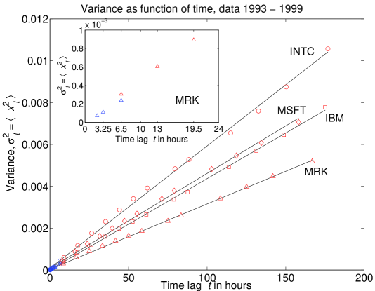
The first result is that we extend to meso time lags a stylized fact known since the 19th century Regnault (quoted in Taqqu ): with a careful definition of time lag $t$, the variance of returns is proportional to $t$.

The second result is that log-linear plots of the EDFs show prominent straight-line (tent-shape) character, i.e. the bulk (about 99%) of the probability distribution of log-return follows an exponential law. The exponential law applies to the central part of EDFs, i.e. not too big log-returns. For the far tails of EDFs, usually associated with power laws at micro time lags, we do not have enough statistically reliable data points at meso lags to make a definite conclusion. Exponential distributions have been reported for some world markets SY ; DY ; Vicente ; India ; Japan ; Germany ; Miranda ; USA and briefly mentioned in the book BP (see Fig. 2.12). However, the exponential law has not yet achieved the status of a stylized fact. Perhaps this is because influential work Stanley1999a ; Stanley1999b has been interpreted as finding that the individual returns of all the major US stocks for micro to macro time lags have the same power law EDFs, if they are rescaled by the volatility.

Figure 5: Top panel: Variance $\langle x_{t}^{2}\rangle$ vs. time lag $t$. Solid lines: Linear fits $\langle x_{t}^{2}\rangle=\theta t$. Inset: Variances for MRK before adjustment for the effective overnight time $T_{n}$. Bottom panel: Log-linear plots of CDFs vs. $x/\sqrt{\theta t}$. Straight dashed lines $-|x|\sqrt{2/\theta t}$ are predicted by the DY formula (29) in the short-time limit. The curves are offset by a factor of 10.

Figure 6: Top panel: Theoretical CDFs for the Heston model plotted vs. $x/\sqrt{\theta t}$. The curves interpolate between the short-time exponential and long-time Gaussian scalings. Bottom panel: Comparison between empirical (points) and the DY theoretical (curves) characteristic functions $\tilde{P}_{t}(k)$.

The Heston model is a plausible diffusion model with stochastic volatility, which reproduces the timelag-variance proportionality and the crossover from exponential distribution to Gaussian. This model was first introduced by Heston, who studied option prices Heston . Later Drăgulescu and Yakovenko (DY) derived a convenient closed-form expression for the probability distribution of returns in this model and applied it to stock indexes from 1 day to 1 year DY . The third result is that the DY formula with three lag-independent parameters reasonably fits the time evolution of EDFs at meso lags.

IV.1 Data analysis and discussion

We analyzed the data from Jan/1993 to Jan/2000 for $27$ Dow companies, but show results only for four large cap companies: Intel (INTC) and Microsoft (MSFT) traded at NASDAQ, and IBM and Merck (MRK) traded at NYSE (please see the appendix for more companies). We use two databases, TAQ to construct the intraday returns and Yahoo database for the interday returns (see Chapter III). The intraday time lags were chosen at multiples of 5 minutes, which divide exactly the 6.5 hours (390 minutes) of the trading day. The interday returns are as described in SY ; DY for time lags from 1 day to 1 month = 20 trading days.

In order to connect the interday and intraday data, we have to introduce an effective overnight time lag $T_{n}$. Without this correction, the open-to-close and close-to-close variances would have a discontinuous jump at 1 day, as shown in the inset of the left panel of Fig. 5. By taking the open-to-close time to be 6.5 hours, and the close-to-close time to be 6.5 hours + $T_{n}$, we find that variance $\langle x_{t}^{2}\rangle$ is proportional to time $t$, as shown in the left panel of Fig. 5. The slope gives us the Heston parameter $\theta$ in Eq. (21). $T_{n}$ is about 2 hours (see Table 1).

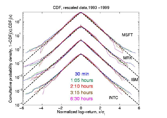
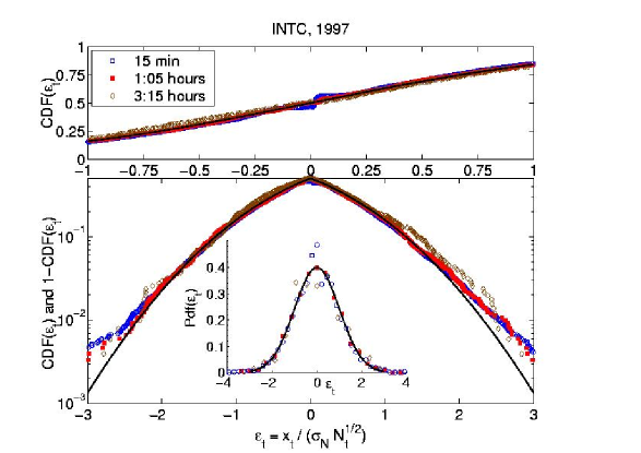
In the right panel of Fig. 5, we show the log-linear plots of the cumulative distribution functions (CDFs) vs. normalized return $x/\sqrt{\theta t}$. The $\makebox{CDF}_{t}(x)$ is defined as $\int_{-\infty}^{x}P_{t}(x^{\prime})\,dx^{\prime}$, and we show $\makebox{CDF}_{t}(x)$ for $x<0$ and $1-\makebox{CDF}_{t}(x)$ for $x>0$. We observe that CDFs for different time lags $t$ collapse on a single straight line without any further fitting (the parameter $\theta$ is taken from the fit in the left panel). More than 99% of the probability in the central part of the tent-shape distribution function is well described by the exponential function. Moreover, the collapsed CDF curves agree with the DY formula (29) $P_{t}(x)\propto\exp(-|x|\sqrt{2/\theta t})$ in the short-time limit for $\alpha=1$ DY , which is shown by the dashed lines.

Table 1: Fitting parameters of the Heston model with $\alpha=1$ for the 1993–1999 data.

$\gamma$ $1/\gamma$ $\theta$ $\mu$ $T_{n}$ ${1\over{\rm hour}}$ hour ${1\over{\rm year}}$ ${1\over{\rm year}}$ hour INTC $1.029$ $0\colon 58$ $13.04\%$ $39.8\%$ $2\colon 21$ IBM $0.096$ $10\colon 25$ $9.63\%$ $35.3\%$ $2\colon 16$ MRK $0.554$ $1\colon 48$ $6.57\%$ $29.4\%$ $1\colon 51$ MSFT $1.284$ $0\colon 47$ $9.06\%$ $48.3\%$ $1\colon 25$

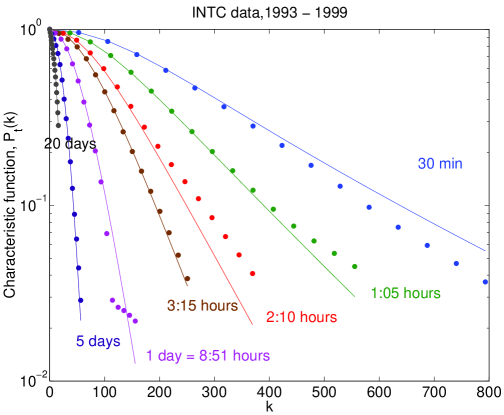
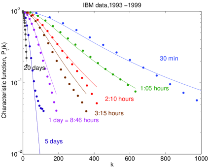
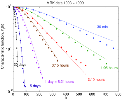
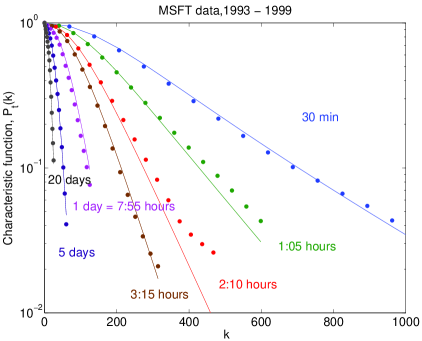
Because the parameter $\gamma$ drops out of the asymptotic Eq. (29), it can be determined only from the crossover regime between short and long times, which is illustrated in the left panel of Fig. 6. We determine $\gamma$ by fitting the characteristic function $\tilde{P}_{t}(k)$, a Fourier transform of $P_{t}(x)$ with respect to $x$. The theoretical characteristic function of the Heston model is $\tilde{P}_{t}(k)=e^{F_{\tilde{t}}(k)}$ (20). The empirical characteristic functions (ECFs) can be constructed from the data series by taking the sum $\tilde{P}_{t}(k)={\rm Re}\sum_{x_{t}}\exp(-ikx_{t})$ over all returns $x_{t}$ for a given $t$ BookCh . Fits of ECFs to the DY formula (20) are shown in the right panel of Fig. 6. The parameters determined from the fits are given in Table 1.

Figure 7: Comparison between the 1993–1999 Intel data (points) and the DY formula (20) (curves) for PDF (top panel) and CDF (bottom panel).

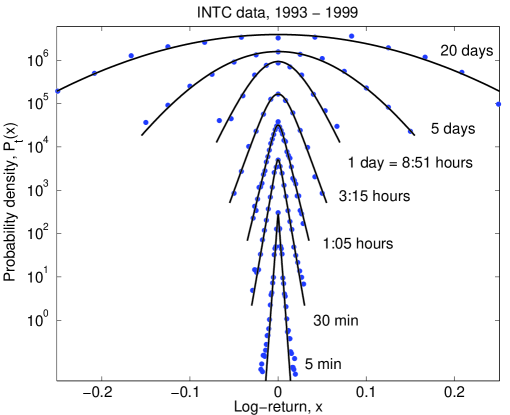
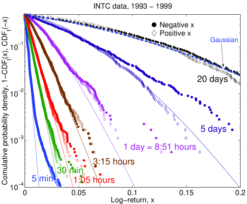
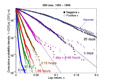
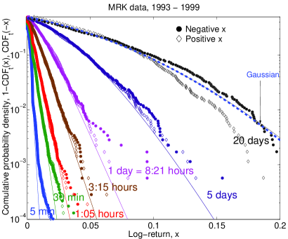
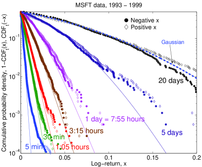
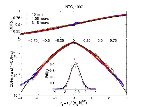
In the left panel of Fig. 7 we compare the empirical PDF $P_{t}(x)$ with the DY formula (20). The agreement is quite good, except for the very short time lag of 5 minutes, where the tails are visibly fatter than exponential. In order to make a more detailed comparison, we show the empirical CDFs (points) with the theoretical DY formula (lines) in the right panel of Fig. 7. We see that, for micro time lags of the order of 5 minutes, the power-law tails are significant. However, for meso time lags, the CDFs fall onto straight lines in the log-linear plot, indicating exponential law. For even longer time lags, they evolve into the Gaussian distribution in agreement with the DY formula (20) for the Heston model. To illustrate the point further, we compare empirical and theoretical data for several other companies in Fig. 8.

In the empirical CDF plots, we actually show the ranking plots of log-returns $x_{t}$ for a given $t$. So, each point in the plot represents a single instance of price change. Thus, the last one or two dozens of the points at the far tail of each plot constitute a statistically small group and show large amount of noise. Statistically reliable conclusions can be made only about the central part of the distribution, where the points are dense, but not about the far tails.

IV.2 Conclusions

We have shown that in the mesoscopic range of time lags, the probability distribution of financial returns interpolates between exponential and Gaussian law. The time range where the distribution is exponential depends on a particular company, but it is typically between an hour and few days. Similar exponential distributions have been reported for the Indian India , Japanese Japan , German Germany , and Brazilian markets Vicente ; Miranda , as well as for the US market SY ; DY ; USA (see also Fig. 2.12 in BP ). The DY formula DY for the Heston model Heston captures the main features of the probability distribution of returns from an hour to a month with a single set of parameters.

Figure 8: Comparison between empirical data (symbols) and the DY formula (20) (lines) for CDF (left panels) and characteristic function (right panels).

V Number of trades and subordination

The concept of subordination has important fundamental and practical implications. From a fundamental point of view, it gives a relation between microstructure of the market and price formation that can be exploited in simulations and modelling Farmer2004 ; Engle2000 ; OHara ; Pohlmeier2003 . From a practical point of view, the subordinator can be identified with the integrated variance $V_{t}$ Bollerslev1996 ; Geman . This would imply a direct measure of the mean square return which could impact pricing and hedging both of options on a particular stock as well as variance swaps and options on the variance.

In this chapter we verify and model the subordination hypothesis as given by Eq. (36). We will restrict our study to intraday Intel data in the year $1997$. We restrict to a year of data because of the nonlinear drift of the number of trades: we would like to minimize this effect (see Fig. LABEL:fig:cunN). We chose Intel because it has been studied by us in Ref. SPY (chapter IV) and it can be modelled well with the Heston model introduced in chapter IV. It is true that it is a highly traded stock, and that is an advantage, since that are a lot of trades in a day and therefore the statistics is better. Therefore smaller stocks should be also checked in the future. The year of $1997$ represents most of what one finds for other years, except perhaps $2000$ and $2001$ which we did not verified because of technical problems (to large data set requires especial computing techniques that should be implemented in the future).

We begin by showing the influence of the discrete nature of the absolute price change in the intraday log-return data. This is rarely pointed out, even though there is a vast literature on intraday log-returns BP ; Stanley1999a ; Stanley1999b ; BS ; MullerBook . This discreteness has to be accounted for when considering subordination, or even when studying intraday returns. It implies that a continuous probability density is only a convenient approximation for some return horizons.

In section V.2, we verify when and for what range of data does subordination apply. We assume that the integrated volatility $V_{t}$ is the random subordinator of a driftless Brownian motion and that $V_{t}$ is proportional to the number of trades $N_{t}$ in an interval of time $t$. We also use tick-by-tick data to check for subordination by constructing the probability density of the log-returns $x_{N}$ after $N$ trades (36).

In section V.3, we model the integrated variance $V_{t}$ with the CIR process introduced in Eq. (38). We present the level of agreement between the data and the theoretical CIR model and we link these results to the distribution of log-returns $x_{t}$.

In the last section, we present a summary of our findings.

V.1 Discrete nature of stock returns

On a tick-by-tick level, price changes are discrete. There is a minimal price change for bid and offers that is set by internal rules of the stock exchange. In the case of Intel in the year of $1997$, the minimal price change was $\$1/8$ for the first part of the year and after June, 24th it became $\$1/16$ Goldstein2000 ; Pruitt2000 . Nevertheless, empirically we find that the smallest price change on realized transactions is $h=\$1/64$ (Fig. 9). This difference is a direct consequence of the mechanism of trading, and we will not study it here (see Ref. Farmer2003Prl ; Farmer2005 ). We note that the minimal price change set by law is clear in Fig. 9, since the most probable price changes are indeed $0$, $\pm 4h=\$1/16$ and $\pm 8h=\$1/8$, according to the rules of the NASDAQ exchange in $1997$.

Our goal in this section is to identify the discrete nature of absolute price changes after $N$ trades ($m_{N}h=S_{n}-S_{n-N}$) in the log-returns after $N$ trades ($x_{N}=ln(S_{n})-ln(S_{n-N})$) and in log-returns after a time-lag $t$ ($x_{t}=ln(S_{T})-ln(S_{T-t})$), since these log-returns are the quantities that we ultimately want to model. We want to point out that the discrete nature of the log-returns for intraday work is generally overlooked but it can influence in the analysis of short returns.

We will refer to minimal price change $h=\$1/64$ as “quantum of price” or simply “quantum” in analogy with quantum mechanics.

The discrete nature of the price change can be used to model the price dynamics starting from a microscopic approach as recently suggested in Engle2000 ; Bollerslev2001 ; Engle1998 ; Pohlmeier2001 . We are interested in the limit where the quantum effect is not noticeable and therefore quantities such as number of trades and returns can be treated as continuous random variables.

Figure 9: Dimensionless absolute returns $m_{N}=(S_{n}-S_{n-N})/h$ for $N$ trades in log linear and linear scale (center and bottom panels respectively). In the top panel we show the difference of the PDFs for $m_{N}$ and $m_{N-1}$ to illustrate the oscillatory nature of the discrete PDF for absolute returns: it evolves from a “pulse” like shape for $N=1$ to a “constant wave” for $N=4000$.

Figure 10: Effect of taking log-returns instead of taking absolute returns. Lower panel shows the probability density of the dimensionless log-returns $x_{N}/h$ conditioned on $m_{N}$, $P(x_{N}/h|m_{N})$. The values concentrated about a multiple of $h$ (upper panel), spread about their respective $h$ value. The vertical color coded lines (lower panel) indicate the $h$ value from which each, equally color coded, $P(x_{N}/h|m_{N})$ originated. The discreteness of $m_{N}$ is removed by taking log-returns since the spread of $P(x_{N}/h|m_{N})$ is larger than $h$.

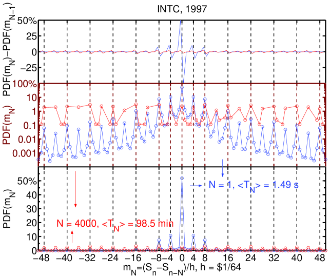
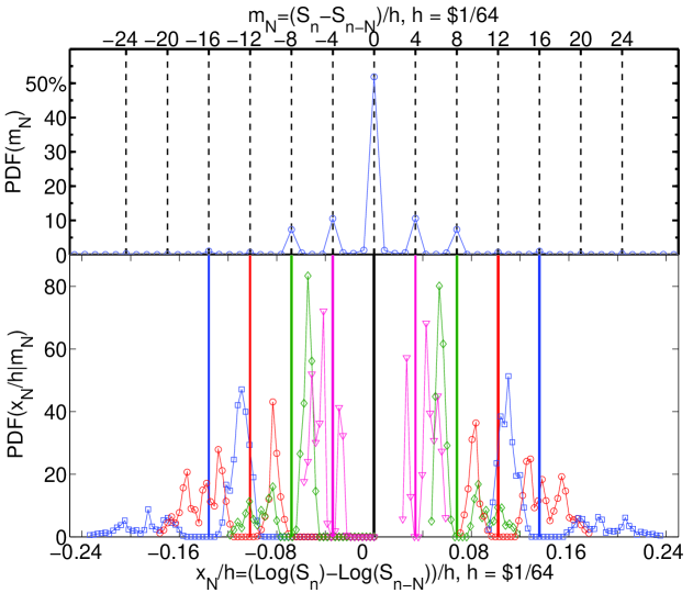
Fig. 9 shows the probability density for the dimensionless absolute price return $m_{N}=(S_{n}-S_{n-N})/h$ after $N$ trades in steps of one quantum $h$. The nature of the tick-by-tick distribution ($N=1$) is considerably different from $N=4000$. More than $50\%$ of the returns are zero for $N=1$, and most of the other returns have a probability of less than $1\%$ except $\pm 4h$ and $\pm 8h$. The probability has a clearly oscillatory nature where multiples of $4h$ are maxima (Fig. 9, top panel). After $4000$ trades the probability distribution for $m_{N}$ has changed into a two level system (Fig. 9). The probability of the most probable $m_{N}$ in $N=1$ have now approximately the same probability. Therefore, the zero return has (after $4000$ trades) a comparable probability to the other probability maxima.

The quantum nature of the price changes is removed by working with log-returns, except for the zero return. Notice that intraday log-returns can be approximated by the ratio Montero

$$x_{N}=\ln{S_{n}}-\ln{S_{n-N}}\approx\frac{S_{n}-S_{n-N}}{S_{n-N}}=\frac{m_{N}}{S_{n-N}/h}.$$ (42)

The log-returns can also be written

$$m_{0,N}h=0$$

$$m_{i,N}h=S_{iN}-S_{(i-1)N},i=1,2,3...$$

$$x_{i,N}=\frac{m_{N}}{\sum_{j=0}^{j=i-1}m_{j,N}+C},C=S_{0}/h,i=1,2,3,...,$$ (43)

where $S_{0}$ is the first open of the year (in the case of Intel 1997, $S_{0}=\$131.75$).

The effect of taking log-returns is illustrated in Fig. 10. For each absolute return $m_{N}$, there is a potentially different denominator $S_{n-N}/h$ (42) composed by a random walk with integer valued steps about a level $C$ (43). Clearly the values of the ratio $x_{N}$ will not be integer. Therefore, the ratio of $m_{N}$ in Eq. (43) spreads the concentrated discrete absolute returns multiple of $h$, around the multiple.

The lower panel of Fig. 10 shows the probability density of $x_{N}/h$ conditioned on $m_{N}$. The conditional probability density $P(x_{N}/h|m_{N})$ illustrates a spread for each $m_{N}$ that is larger than $h$. This spread is enough to mix the discreteness with exception of $m_{N}=0$.

The quality of such a mixture can be seen in Fig. 11 and Fig. 12. Even though the cumulative density function for $x_{N}$ is practically continuous (even for $N=1$) with exception of $x_{N}=0$, the stepwise nature of $m_{N}$ can be easily recognized up to $N=1000$ (Fig. 12). The oscillations in the cumulative density functions for $x_{N}$ are centered about the discrete steps of the cumulative density function of $m_{N}$.

Figure 11: Cumulative probability density for both dimensionless log-returns, $x_{N}/h$ (black line), and dimensionless absolute returns, $m_{N}$ (blue symbols). Even though the discreteness of $m_{N}$ is removed with exception of $x_{N}=0$, the signature of such discreteness is still visible. Notice the stepwise nature of the black line.

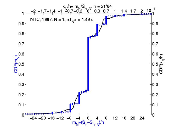
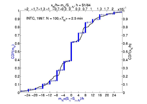
The discrete quantum effect at $m_{N}=0$ is quite persistent, but it can be neglected for returns $x_{N}$ with large number of trades $N$ (for instance $N=4000$). Empirically, it appears that the criteria for neglecting the $m_{N}=0$ effect is that the probability of having $m_{N}=0$ is of the same order of magnitude as the probability of having any other $m_{N}$ (Fig.9). For Intel $1997$ this transition starts approximately at $N=1000$.

Figure 12: Cumulative probability density for both dimensionless log-returns, $x_{N}/h$, and dimensionless absolute returns, $m_{N}$. When $N$ increases the CDF becomes progressively less oscillatory and the discrete nature of the underlying absolute returns becomes less clear.

Figure 13: Cumulative probability density for $x_{t}/h$ with $t=5$ minutes. The discreteness at zero persists from $x_{N}/h$ as well as the oscillation (stepwise nature) of the CDF.

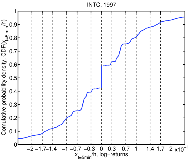
The effect of data discreteness is also present in the log-return $x_{t}$ of time lag $t$. From the log-return $x_{t}$, we can construct $x_{N}$ by conditioning on the number of trades $N$ present in $t$ ($N_{t}$). The opposite is also true, by conditioning on $t$ we can construct $x_{t}$ from $x_{N}$. Therefore some of the discrete effects that are present in $x_{N}$ will be present in $x_{t}$. As an example consider $5$ minute log-returns. The average number of trades is $\langle N_{t=5min}\rangle=200\pm 184$. Because of the reciprocity in constructing the PDF for $x_{t}$ from $x_{N}$ (and vice-versa) by conditioning, this shows that in the composition of $x_{t=5min}$, there is a wide range of $x_{N}$ for which the discrete features can not be ignored (clear oscillations and large probability for $x_{t}=0$). If we approximate the PDF of $N_{t=5min}$ by a Gaussian distribution, we would have in $x_{t=5min}$, with the highest probability, $N_{t=5min}=200$. Therefore some fraction of $x_{N}=200$ will be sampled when we construct the probability of $x_{t=5min}$ by conditioning, these returns clearly have a lot of discrete features (Fig. 12) and these features will pass to $x_{t=5min}$.

Fig. 13 shows the oscillatory stepwise cumulative probability density and also the special nature of $x_{t=5min}=0$ for the cumulative probability density of $x_{t=5min}$. Compare this figure with Fig. 11 and Fig. 12. These features originate from $x_{N}$ and represent small flat portions in the probability density function.

Finally, from the sequence of Figs. 11 and 12 and the correspondence between $x_{N}$ and $x_{t}$, we can conclude that the discrete effects become negligible for a time lag $t>1$ hour.

V.2 Verifying subordination with intraday data

The hypothesis of subordination introduced by Clark Clark has had a strong economical implication, and following his work there is a vast body of theoretical and empirical work which addresses the issue Smith1994 ; Manganelli2000 ; Ane2000 ; Stanley2000 ; Farmer2004 . Similar to the work of Refs. Ane2000 ; Stanley2000 , we verify for subordination considering integrated variance $V_{t}$, constructed from the number of trades $N_{t}$, to be the subordinator of a Brownian motion.

Due to the discrete nature of the distribution of intraday returns presented in section (V.1), we can only talk about subordination as formulated in equation (36) after the discrete effects become small. In what follows, we will take all time lags even those where the discrete effects are large. Nevertheless, we will see that the best subordination will take place for time lags for which discrete effects can be ignored.

Figure 14: Variance of the log-return $x_{N}$ for $N=1$ to $N=10000$.

Figure 15: Variance of the demean log-return $x_{t}$ for intraday time lags $t$.

Figure 16: Average number of trades in an intraday interval $t$.

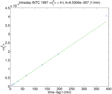
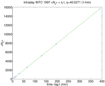
The first implication of subordination can be verified with the use of moments given by equations (33) and (35). Figs. 16 and 16 show the linear time relation for both the variance of $x_{t}$ and the mean of $N_{t}$ as expected from equation (33). Furthermore, since we are assuming a Brownian motion with stochastic variance given by the number of trades, log-returns $x_{N}$ after $N$ trades should be Gaussian distributed with variance $\langle x_{N}^{2}\rangle=\sigma_{N}^{2}N$. Fig. 16 shows the linear relation of $\langle x_{N}^{2}\rangle$ vs. $N$. The implied consistency between the slope values in Figs. 16, 16 and 16 required by subordination is

$$\langle x_{t}^{2}\rangle=\theta t=\sigma_{N}^{2}\langle N_{t}\rangle=\sigma_{N}^{2}\eta t\,\Rightarrow\,\theta=\sigma_{N}^{2}\eta.$$ (44)

Using expression (44), the difference between $\theta$ measured (Fig.16) and $\theta=\eta\sigma_{N}^{2}$ from Fig. 16 and Fig. 16 is less than $1\%$.

Figure 17: Cumulative probability density for the demean and standard deviation (STD) normalized $x_{N}$ log-returns (color coded solid curves), compared to the Gaussian distribution of mean zero and STD one (dashed curve). From small $N$ to large $N$, there is a progressive agreement with the Gaussian with best agreement between $N=3500$ and $N=4500$. While smaller values of $N$ have CDFs above the Gaussian, larger values are below the Gaussian.

Figure 18: Skewness and excess kurtosis (labelled as ”kurtosis” in the figure) as a function of $N$ for the normalized log-returns $x_{N}$ in Fig. 17. For a Gaussian distribution the skewness is zero and the excess kurtosis is also zero. As the number of trades (ticks) $N$ increase the skewness and excess kurtosis become zero. The probability density for $x_{N}$ can be well approximated by a Gaussian for $N>2500$, since both skewness and excess kurtosis are small.

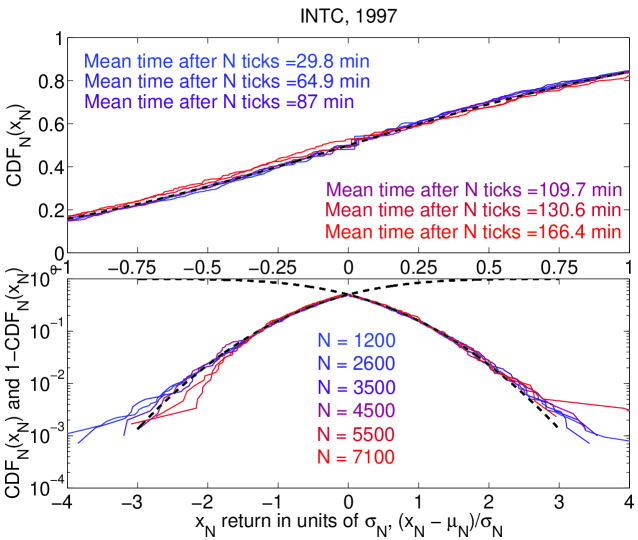
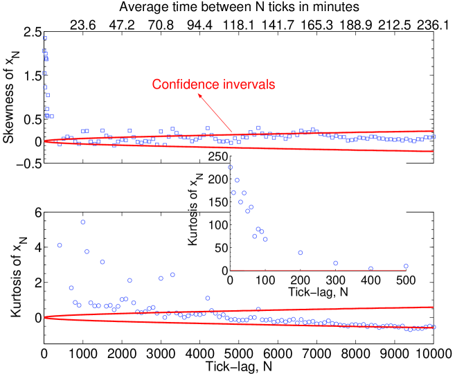
In order to find a time and a return range where subordination takes place, we look at the data in $3$ different ways. First, using tick-by-tick data, we construct the distribution of the log-return $x_{N}$ after $N$ trades. $x_{N}$ should be Normal distributed with mean zero and standard deviation $\sigma_{N}\sqrt{N}$. We also present the $N$ dependence of the skewness ($\langle x_{N}^{3}\rangle/(\langle x_{N}^{2}\rangle^{3/2})$) and excess kurtosis ($\langle x_{N}^{4}\rangle/(\langle x_{N}^{2}\rangle^{2})-3$) of $x_{N}$ in Fig. 18.

Second, using $t$ minute returns $x_{t}$ and the number of trades $N_{t}$ in the same $t$ interval, we construct the time series

$$\epsilon_{t}=\frac{x_{t}}{\sqrt{V_{t}}},\,V_{t}=\sigma_{N}^{2}N_{t},$$ (45)

where $V_{t}$ is the integrated variance in an interval $t$ and $\sigma_{N}$ is the proportionality constant that converts number of trades $N_{t}$ into variance. If indeed subordination holds, $\epsilon_{t}$ is Normal distributed with mean zero and standard deviation one, due to the central limit theorem FellerBook ; Stanley2000 .

Figure 19: Cumulative density function (CDF) for $\epsilon_{t}$ as defined in equation (45) for three different $t$ compared to the Gaussian (solid line). The parameters $\sigma_{N}$ in (45) is chosen for the best agreement between the Gaussian and the data.

Figure 20: Cumulative density function (CDF) for $\epsilon_{t}$ as defined in equation (45) for three different $t$ compared to the Gaussian (solid line). Contrary to Fig. 20, the parameter $\sigma_{N}$ in equation (45) is found using Fig. 16. Notice that the Gaussian lies above the data in the tails.

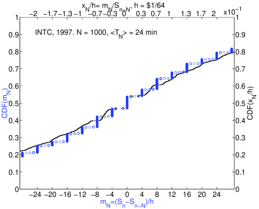
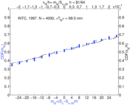
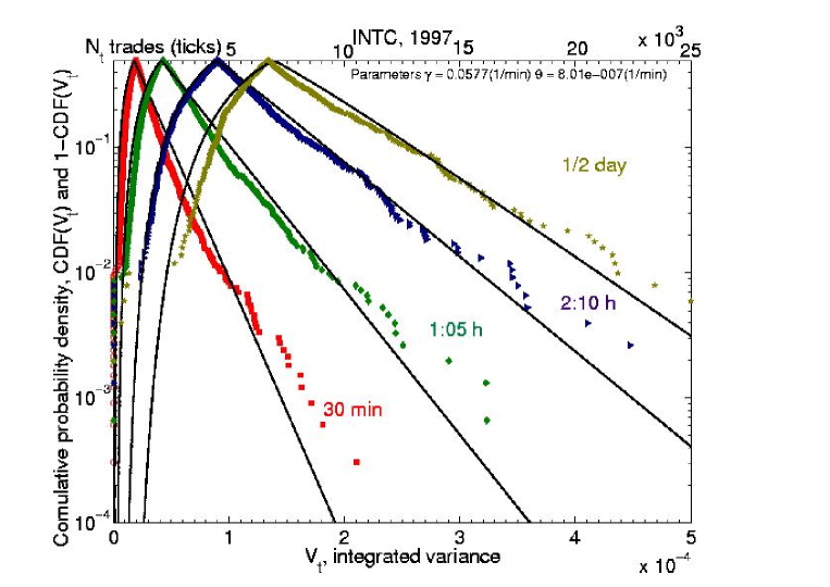
Finally, we check subordination by numerically calculating the probability mixture equation (36). We construct the probability density function of the number of trades $N_{t}$ inside a time interval $t$ by binning the time series of $N_{t}$. The choice for binwidth is according to Ref. Scott . However, the result appears independent of binwidth as long as the binwidth chosen is not too large. The cumulative probability density function for the measured $x_{t}$ and the non-parametric reconstructed $x_{t}^{\prime}$ are shown in Fig. 21.

Figure 21: Cumulative distribution of the stock returns $x_{t}$ compared to the reconstructed cumulative distribution function (black lines) by randomizing the variance $V_{t}$ of a Gaussian distribution. The probability of $V_{t}$ is constructed by binning the number of trades, and this probability is used non-parametrically in the integral (36). The solid lines have parameter $\sigma_{N}$ chosen in order to minimize the least square error between the empirical $x_{t}$ distribution and reconstructed variance changed Brownian motion (36). The dashed line has $\sigma_{N}$ found from Fig. 16.

The distributions in Fig. 17, Fig. 20 and Fig. 21(solid line) show an agreement of approximately $85\%$ of the data with the subordination hypothesis for time lags above $t>1$ hour or $N>2500$ (Fig. 18). However, the subordination is clearly bad for times close to one day ($t=6.5$ hours), where we do not have enough data (253 points) to draw meaningful conclusions.

Notice the clear disagreement above $2$ standard deviations (STD) as well as at zero in Fig. 17 and Fig. 20. The deviations at zero are due to the discrete nature of the data (section V.1) while the deviations above $2$ STD show that the subordination hypothesis can not explain the large changes in returns Farmer2004 .

For Fig. 20 and Fig. 21(solid line), $\sigma_{N}^{2}=2\times 10^{-8}$ is found to give the best agreement between the measured data and the reconstructed data. For Fig. 17, Fig. 20 and Fig. 21(dashed line), $\sigma_{N}^{2}=2.39\times 10^{-8}$ is found from Fig. 16. Notice that the higher $\sigma_{N}$ in Fig. 20 and Fig. 21 (dashed lines) seems to indicate an overestimation of $\sigma_{N}$, since the curves constructed by subordination are generally above the data.

The lower value of $\sigma_{N}^{2}$ for Fig. 20 and Fig. 21 (solid line) leads to a violation of relation (44). The difference between measured $\theta$ in Fig. 16 and the one calculated from $\eta\sigma_{N}^{2}$ is now of approximately $16\%$. In order to verify the origin of such difference, we remove $8\%$ of the largest log-return $x_{t}$ data on both tails (ignore $8\%$ of the largest $x_{t}$ on the positive and negative tail for all time lags $t$ used), a total of $16\%$ of the data. We find now a $\theta\approx 8.01\times 10^{-7}$. This new $\theta$ does not violate relation (44) with $\sigma_{N}^{2}=2\times 10^{-8}$ and reconfirms that subordination with $V_{t}=\sigma_{N}^{2}N_{t}$ is unable to explain large changes ($>85\%$) in the log-returns $x_{t}$. This reconfirmation arises because we had to ignore $16\%$ of the data in the tails to reduce $\theta$. Dropping $16\%$ of the tails is equivalent to looking only at the center $\approx 85\%$ of the data and saying that subordination is only valid of it.

V.3 Models for the subordinator

Having verified that a Brownian motion subordinated to the number of trades $N_{t}$ via $V_{t}$ can describe approximately $85\%$ of the return data for time lags larger than $1$ hour (or, if one ignores discreetness effects such as the zero return effect, larger than $30$ minutes), we can model $V_{t}$ instead of modelling $x_{t}$.

In this section, we verify the quality of modelling $V_{t}$ with a CIR process as given in section (II.2). We present the quality of the CIR fit for Intel in the year $1997$. We also show that the quality of the Heston fit to $x_{t}$ with parameters from the $V_{t}$ CIR fit is consistent with the quality of the subordination: we are able to model most of the central $85\%$ of the $x_{t}$ distribution.

Figure 22: Empirical probability density function for the number of trades (ticks) $N_{t}$ or integrated variance $V_{t}=\sigma_{N}^{2}N_{t}$, compared to the least square fit with the CIR formula (38). Curves are offset by a factors of 10.

Figure 23: Cumulative distribution function (CDF) for the number of trades $N_{t}$ and integrated variance $V_{t}$ compared to the CIR fit (solid lines). The $CDF(V_{t})$ goes from $0$ to $0.5$. $1-CDF(V_{t})$ goes from $0.5$ to $0$. The lower tail ($V_{t}:0->0.5$) of the $CDF$ is to the left and the upper tail ($V_{t}:0.5->0$) to the right of $0.5$ for each time $t$ curve.

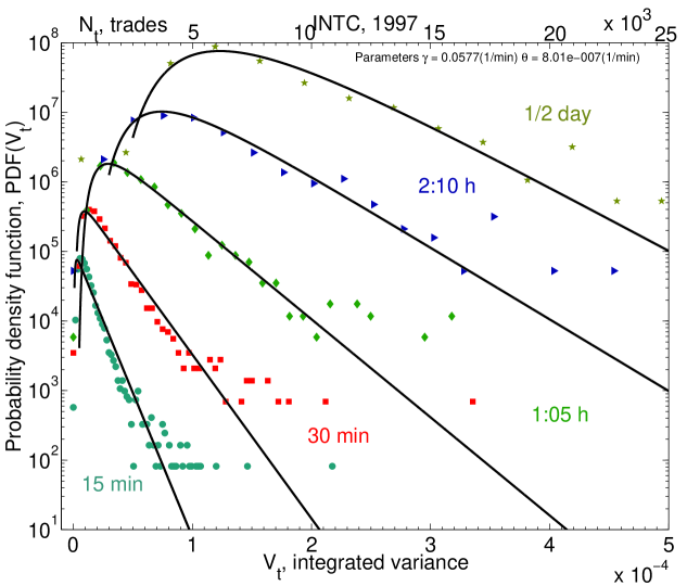
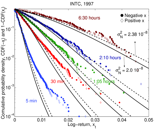
Due to previous studies with intraday log-returns SPY (see also chapter IV), we assume $\alpha=1$ for the simplified CIR model in equation (38). The parameter $\theta$ is found from the relation $\theta=\eta\sigma_{N}^{2}$ (44). The remaining parameter $\gamma$ is found by fitting the empirical $PDF(V_{t})$ for time lags $t=1\colon 05$ hours and $t=2\colon 10$ hours simultaneously. The regular quality of such a fit is shown in Figs. 22 and 23. The theoretical CIR lines are above the data (Fig. 23). Furthermore, the time dependence of the theoretical PDF and CDF only approximately follow the data. For times below $1$ hour the probability maximum of the empirical distribution is to the left of the theoretical distribution and for times above $1$ hour to the right.

Figure 24: Variance of the integrated variance $\langle V_{t}^{2}-\langle V_{t}\rangle^{2}\rangle$ for different time lags $t$ for the data (circles) compared to the theoretical CIR variance given in equation (41) (solid black line). For comparison the best power-law fit $\langle V_{t}^{2}-\langle V_{t}\rangle^{2}\rangle\propto t^{1.77}$ is shown (solid red line).

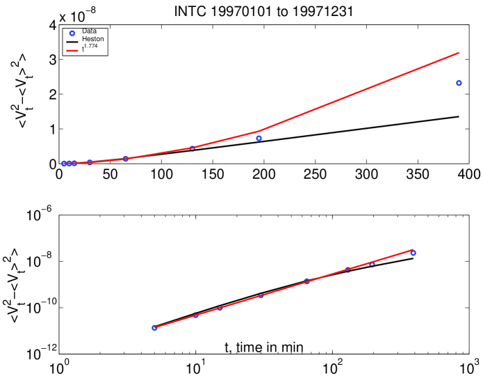
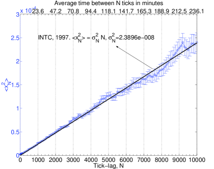
The results shown in Figs. 22 and 23 indicate that the CIR is only approximately valid. The quality can be further assessed by constructing the variance of the $V_{t}$ as a function of the time lag $t$. Fig. 24 shows that the theoretical variance given in equation (41) is only approximately correct. Nevertheless from equation (33), we know that the variance of $V_{t}$ corresponds to the kurtosis of $x_{t}$. This indicates that even though $V_{t}$ can not be modelled well (not even the second moment) the implication of that is only important to the fourth and higher moments in the log-returns $x_{t}$.

Figure 25: Probability distribution function for the log-returns $x_{t}$ compared to the Heston model (dashed and solid lines). The two lines represent a different set of parameters. The solid line has parameters $\theta$ from Fig. 16 and $\gamma$ is found directly by fitting $x_{t}$. The dashed lines has $\theta=\sigma_{N}^{2}\eta$ with $\sigma_{N}^{2}$ from Fig. 21(solid lines) and Fig. 20 and $\eta$ from Fig. 16. The parameter $\gamma$ is then found by fitting the probability density of $V_{t}$. Curves are offset by factors of 10.

Figure 26: Cumulative probability density of $x_{t}$ compared to the Heston model. Theoretical lines (dashed and solid) are constructed by integrating the theoretical probability density functions shown in Fig. 25. The two theoretical lines represent a different set of parameter. The solid line has parameters $\theta$ from Fig. 16 and $\gamma$ is found directly by fitting $x_{t}$. The dashed lines has $\theta=\sigma_{N}^{2}\eta$ with $\sigma_{N}^{2}$ from Fig. 21(solid lines) and Fig. 20 and $\eta$ from Fig. 16. The parameter $\gamma$ is then found by fitting the probability density of $V_{t}$. Notice that the solid black line clearly gives a better fit to the data.

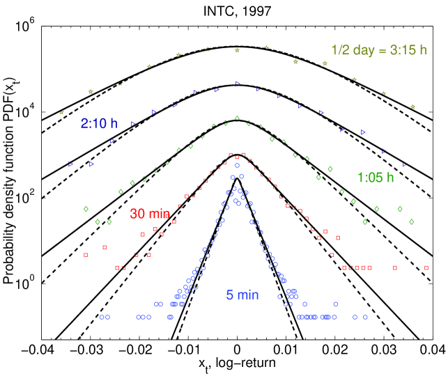
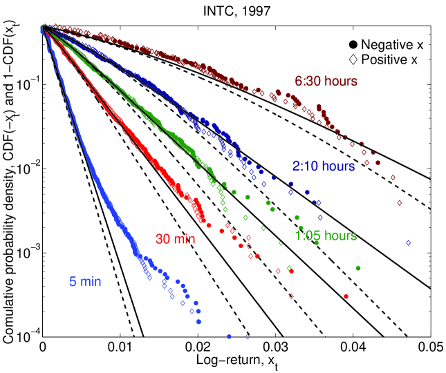
To verify the quality of the parameters found by fitting the subordinator, $V_{t}$, in explaining the log-returns, $x_{t}$, we present Figs. 25 and 26. The empirical PDF (25) and CDF (26) for $x_{t}$ show that the corresponding Heston model (dashed black lines), constructed with parameters found by fitting CIR to the probability density of $V_{t}$, is able to fit only the center of the empirical distributions of $x_{t}$ ($\approx 80\%-85\%$) at $t=65,130$ minutes (Fig. 26).

To recheck the consistency of the subordination approach, we fit the empirical PDF of $x_{t}$ directly with the Heston model (20). We proceed in similar fashion to the fitting procedure in chapter IV. We assume $\alpha=1$ and take $\theta=8.01\times 10^{-7}$. The parameter $\theta$ was found from the relation $\theta=\sigma_{N}^{2}\eta$ (44), where $\eta$ is found from Fig. 16 and $\sigma_{N}^{2}$ is given such that the subordination in Figs. 20 and 21 is the best possible. Finally, we fit the empirical PDFs (Fig. 25) for the parameter $\gamma$. Therefore, we are effectively only fitting $\gamma$, since all the other parameters are the same used in the $V_{t}$ fit (Fig. 22). We find that the $\gamma$ found from fitting the empirical PDF of $x_{t}$ directly, is of the same order of magnitude as with the one found by fitting the empirical PDF of $V_{t}$ (0.05 from $x_{t}$ and 0.06 from $V_{t}$). This shows, that the subordination indeed captures most of the information for the center of the distribution, since fitting $V_{t}$ or $x_{t}$ for $\gamma$ is equivalent.

Notice that the agreement of the theoretical Heston model curves, constructed with parameters from the $V_{t}$ fit, is practically identical to the agreement found in Fig. 21(solid lines) between the CDF of $x_{t}$ and the CDF constructed by subordination using the non-parametric binned probability density of $V_{t}$ as the variance of a Gaussian random walk (36). The information content in the number of trades and therefore in the integrated variance distribution is almost all captured by CIR, even with a regular fit quality (Fig. 23). This last point implies that even if we had a better fit to the distribution of $V_{t}$, the increase in the fitting quality of the log-returns will not be substantial.

A substantial increase in the fitting quality of the empirical PDF and CDF of the log-returns in Figs. 25 and 26 is attained if one fits the empirical PDF of $x_{t}$ directly with $\theta=9.53\times 10^{-7}$ given in Fig. 16. This amounts to take $\sigma_{N}^{2}$ as given by Fig. 16 and $\eta$ by Fig. 16, such that relation (44) is still valid. The parameter $\gamma=0.02$ for the black solid lines in Fig. 26 is also considerably different from $\gamma=0.06$, found by fitting the empirical PDF of $V_{t}$ and using $\theta=8.01\times 10^{-7}$ such that $\sigma_{N}^{2}$ is the best fit value for the subordination in Figs. 21(solid line) and 20. The substantial increase in the fitting quality for $x_{t}$, reemphasizes that the number of trades are only able to describe the center of the distribution of log-returns (section V.2).

V.4 Conclusion

We have studied the discrete nature of the probability distribution of absolute returns that arises from the minimal discrete price change for bid and offers allowed by the stock exchange. We have shown that such discrete nature implies that the probability distributions of log-returns for intraday time lags are only approximately continuous. The continuous approximation becomes good for returns with time lags longer than $1$ hour.

We have shown that, using the integrated volatility $V_{t}=\sigma_{N}^{2}N_{t}$ derived from the number of trades $N_{t}$ as the subordinator of a driftless Brownian motion (36), we are able to describe the center ($\approx 85\%$) of the distribution of log-returns $x_{t}$ for time lags $t>1$ hour and smaller than $t<1$ day. The upper limit is restricted by the number of data points we have, since we are working with only one year of data.

We also have shown that the CIR process is only able to approximately describe the distribution function for $V_{t}$. However, this approximate description is already enough for the corresponding Heston model to fit the log-returns $x_{t}$ with approximately the maximum quality that the subordination allows ($\approx 80\%-85\%$).

Finally, a direct fit to the log-returns $x_{t}$ with the Heston model results in a considerable increase in the fitting quality. This reemphasizes that the process of subordination, as implied by the empirical probability density of $V_{t}$, is only able to explain the center of the distribution of returns.

VI Income distribution

Attempts to apply the methods of exact sciences, such as physics, to describe a society have a long history Ball . At the end of the 19th century, Italian physicist, engineer, economist, and sociologist Vilfredo Pareto suggested that income distribution in a society is described by a power law Pareto . Modern data indeed confirm that the upper tail of income distribution follows the Pareto law Champernowne ; Aoki ; Souma ; Gallegati ; Australia . However, the majority of the population does not belong there, so characterization and understanding of their income distribution remains an open problem. Drăgulescu and Yakovenko Yakovenko-money proposed that the equilibrium distribution should follow an exponential law analogous to the Boltzmann-Gibbs distribution of energy in statistical physics. The first factual evidence for the exponential distribution of income was found in Ref. Yakovenko-income . Coexistence of the exponential and power-law parts of the distribution was recognized in Ref. Yakovenko-wealth . However, these papers, as well as Ref. Yakovenko-survey , studied the data only for a particular year. Here we analyze temporal evolution of the personal income distribution in the USA during 1983–2001. We show that the US society has a well-defined two-income-class structure. The majority of population (97–99%) belongs to the lower income class and has a very stable in time exponential (“thermal”) distribution of income. The upper income class (1–3% of population) has a power-law (“superthermal”) distribution, whose parameters significantly change in time with the rise and fall of the stock market. Using the principle of maximal entropy, we discuss the concept of equilibrium inequality in a society and quantitatively show that it applies to the bulk of the population.

VI.1 Data analysis and discussion

Most of academic and government literature on income distribution and inequality Kakwani ; Cowell ; Atkinson ; Petska does not attempt to fit the data by a simple formula. When fits are performed, usually the log-normal distribution Gibrat is used for the lower part of the distribution Souma ; Gallegati ; Australia . Only recently the exponential distribution started to be recognized in income studies Nirei ; Mimkes , and models showing formation of two classes started to appear West ; Wright .

Let us introduce the probability density $P(r)$, which gives the probability $P(r)\,dr$ to have income in the interval $(r,r+dr)$. The cumulative probability $C(r)=\int_{r}^{\infty}dr^{\prime}P(r^{\prime})$ is the probability to have income above $r$, $C(0)=1$. By analogy with the Boltzmann-Gibbs distribution in statistical physics Yakovenko-money ; Yakovenko-income , we consider an exponential function $P(r)\propto\exp(-r/T)$, where $T$ is a parameter analogous to temperature. It is equal to the average income $T=\langle r\rangle=\int_{0}^{\infty}dr^{\prime}r^{\prime}P(r^{\prime})$, and we call it the “income temperature.” When $P(r)$ is exponential, $C(r)\propto\exp(-r/T)$ is also exponential. Similarly, for the Pareto power law $P(r)\propto 1/r^{\alpha+1}$, $C(r)\propto 1/r^{\alpha}$ is also a power law.

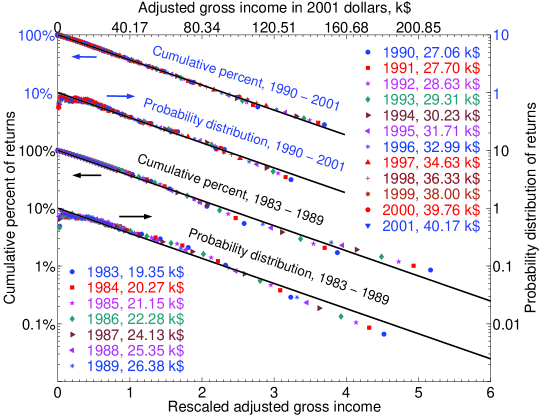
We analyze the data IRS on personal income distribution compiled by the Internal Revenue Service (IRS) from the tax returns in the USA for the period 1983–2001 (presently the latest available year). The publicly available data are already preprocessed by the IRS into bins and effectively give the cumulative distribution function $C(r)$ for certain values of $r$. First we make the plots of $\log C(r)$ vs. $r$ (the log-linear plots) for each year. We find that the plots are straight lines for the lower 97–98% of population, thus confirming the exponential law. From the slopes of these straight lines, we determine the income temperatures $T$ for each year. In Fig. 28, we plot $C(r)$ and $P(r)$ vs. $r/T$ (income normalized to temperature) in the log-linear scale. In these coordinates, the data sets for different years collapse onto a single straight line. (In Fig. 28, the data lines for 1980s and 1990s are shown separately and offset vertically.) The columns of numbers in Fig. 28 list the values of the annual income temperature $T$ for the corresponding years, which changes from 19 k$ in 1983 to 40 k$ in 2001. The upper horizontal axis in Fig. 28 shows income $r$ in k$ for 2001.

Figure 27: Cumulative probability $C(r)$ and probability density $P(r)$ plotted in the log-linear scale vs. $r/T$, the annual personal income $r$ normalized by the average income $T$ in the exponential part of the distribution. The IRS data points are for 1983–2001, and the columns of numbers give the values of $T$ for the corresponding years.

centerline

Figure 28: Log-log plots of the cumulative probability $C(r)$ vs. $r/T$ for a wider range of income $r$.

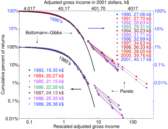
In Fig. 28, we show the same data in the log-log scale for a wider range of income $r$, up to about $300T$. Again we observe that the sets of points for different years collapse onto a single exponential curve for the lower part of the distribution, when plotted vs. $r/T$. However, above a certain income $r_{*}\approx 4T$, the distribution function changes to a power law, as illustrated by the straight lines in the log-log scale of Fig. 28. Thus we observe that income distribution in the USA has a well-defined two-class structure. The lower class (the great majority of population) is characterized by the exponential, Boltzmann-Gibbs distribution, whereas the upper class (the top few percent of population) has the power-law, Pareto distribution. The intersection point of the exponential and power-law curves determines the income $r_{*}$ separating the two classes. The collapse of data points for different years in the lower, exponential part of the distribution in Figs. 28 and 28 shows that this part is very stable in time and, essentially, does not change at all for the last 20 years, save for a gradual increase of temperature $T$ in nominal dollars. We conclude that the majority of population is in statistical equilibrium, analogous to the thermal equilibrium in physics. On the other hand, the points in the upper, power-law part of the distribution in Fig. 28 do not collapse onto a single line. This part significantly changes from year to year, so it is out of statistical equilibrium. A similar two-part structure in the energy distribution is often observed in physics, where the lower part of the distribution is called “thermal” and the upper part “superthermal” superthermal .

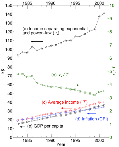
Temporal evolution of the parameters $T$ and $r_{*}$ is shown in Fig. 29. We observe that the average income $T$ (in nominal dollars) was increasing gradually, almost linearly in time, and doubled in the last twenty years. In Fig. 29, we also show the inflation coefficient (the consumer price index CPI from Ref. CPI ) compounded on the average income of 1983. For the twenty years, the inflation factor is about 1.7, thus most, if not all, of the nominal increase in $T$ is inflation. Also shown in Fig. 29 is the nominal gross domestic product (GDP) per capita CPI , which increases in time similarly to $T$ and CPI. The ratio $r_{*}/T$ varies between 4.8 and 3.2 in Fig. 29.

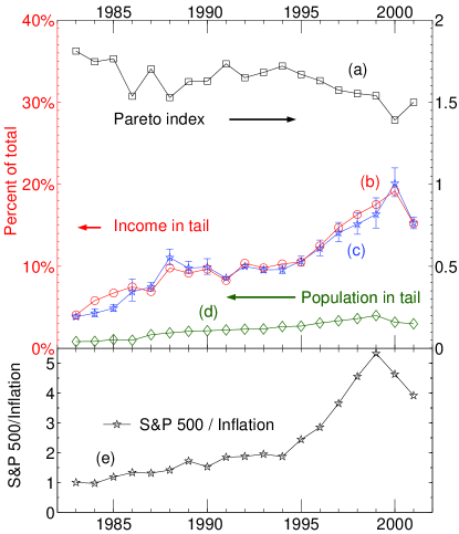
In Fig. 30, we show how the parameters of the Pareto tail $C(r)\propto 1/r^{\alpha}$ change in time. Curve (a) shows that the power-law index $\alpha$ varies between 1.8 and 1.4, so the power law is not universal. Because a power law decays with $r$ more slowly than an exponential function, the upper tail contains more income than we would expect for a thermal distribution, hence we call the tail “superthermal” superthermal . The total excessive income in the upper tail can be determined in two ways: as the integral $\int_{r_{*}}^{\infty}dr^{\prime}r^{\prime}P(r^{\prime})$ of the power-law distribution, or as the difference between the total income in the system and the income in the exponential part. Curves (c) and (b) in Fig. 30 show the excessive income in the upper tail, as a fraction $f$ of the total income in the system, determined by these two methods, which agree with each other reasonably well. We observe that $f$ increased by the factor of 5 between 1983 and 2000, from 4% to 20%, but decreased in 2001 after the crash of the US stock market. For comparison, curve (e) in Fig. 30 shows the stock market index S&P 500 divided by inflation. It also increased by the factor of 5.5 between 1983 and 1999, and then dropped after the stock market crash. We conclude that the swelling and shrinking of the upper income tail is correlated with the rise and fall of the stock market. Similar results were found for the upper income tail in Japan in Ref. Aoki . Curve (d) in Fig. 30 shows the fraction of population in the upper tail. It increased from 1% in 1983 to 3% in 1999, but then decreased after the stock market crash. Notice, however, that the stock market dynamics had a much weaker effect on the average income $T$ of the lower, “thermal” part of income distribution shown in Fig. 29.

Figure 29: Temporal evolution of various parameters characterizing income distribution.

Figure 30: (a) The Pareto index $\alpha$ of the power-law tail $C(r)\propto 1/r^{\alpha}$. (b) The excessive income in the Pareto tail, as a fraction $f$ of the total income in the system, obtained as the difference between the total income and the income in the exponential part of the distribution. (c) The tail income fraction $f$, obtained by integrating the Pareto power law of the tail. (d) The fraction of population belonging to the Pareto tail. (e) The stock-market index S&P 500 divided by the inflation coefficient and normalized to 1 in 1983.

For discussion of income inequality, the standard practice is to construct the so-called Lorenz curve Kakwani . It is defined parametrically in terms of the two coordinates $x(r)$ and $y(r)$ depending on the parameter $r$, which changes from 0 to $\infty$. The horizontal coordinate $x(r)=\int_{0}^{r}dr^{\prime}P(r^{\prime})$ is the fraction of population with income below $r$. The vertical coordinate $y(r)=\int_{0}^{r}dr^{\prime}r^{\prime}P(r^{\prime})/\int_{0}^{\infty}dr^{\prime}r^{\prime}P(r^{\prime})$ is the total income of this population, as a fraction of the total income in the system. Fig. 31 shows the data points for the Lorenz curves in 1983 and 2000, as computed by the IRS Petska . For a purely exponential distribution of income $P(r)\propto\exp(-r/T)$, the formula $y=x+(1-x)\ln(1-x)$ for the Lorenz curve was derived in Ref. Yakovenko-income . This formula describes income distribution reasonably well in the first approximation Yakovenko-income , but visible deviations exist. These deviations can be corrected by taking into account that the total income in the system is higher than the income in the exponential part, because of the extra income in the Pareto tail. Correcting for this difference in the normalization of $y$, we find a modified expression Yakovenko-survey for the Lorenz curve

$$y=(1-f)[x+(1-x)\ln(1-x)]+f\Theta(x-1),$$ (46)

where $f$ is the fraction of the total income contained in the Pareto tail, and $\Theta(x-1)$ is the step function equal to 0 for $x<1$ and 1 for $x\geq 1$. The Lorenz curve (46) experiences a vertical jump of the height $f$ at $x=1$, which reflects the fact that, although the fraction of population in the Pareto tail is very small, their fraction $f$ of the total income is significant. It does not matter for Eq. (46) whether the extra income in the upper tail is described by a power law or another slowly decreasing function $P(r)$. The Lorenz curves, calculated using Eq. (46) with the values of $f$ from Fig. 30, fit the IRS data points very well in Fig. 31.

Figure 31: Main panel: Lorenz plots for income distribution in 1983 and 2000. The data points are from the IRS Petska , and the theoretical curves represent Eq. (46) with $f$ from Fig. 30. Inset: The closed circles are the IRS data Petska for the Gini coefficient $G$, and the open circles show the theoretical formula $G=(1+f)/2$.

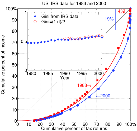
The deviation of the Lorenz curve from the diagonal in Fig. 31 is a certain measure of income inequality. Indeed, if everybody had the same income, the Lorenz curve would be the diagonal, because the fraction of income would be proportional to the fraction of population. The standard measure of income inequality is the so-called Gini coefficient $0\leq G\leq 1$, which is defined as the area between the Lorenz curve and the diagonal, divided by the area of the triangle beneath the diagonal Kakwani . It was calculated in Ref. Yakovenko-income that $G=1/2$ for a purely exponential distribution. Temporal evolution of the Gini coefficient, as determined by the IRS Petska , is shown in the inset of Fig. 31. In the first approximation, $G$ is quite close to the theoretically calculated value 1/2. The agreement can be improved by taking into account the Pareto tail, which gives $G=(1+f)/2$ for Eq. (46). The inset in Fig. 31 shows that this formula very well fits the IRS data for the 1990s with the values of $f$ taken from Fig. 30. We observe that income inequality was increasing for the last 20 years, because of swelling of the Pareto tail, but started to decrease in 2001 after the stock market crash. The deviation of $G$ below 1/2 in the 1980s cannot be captured by our formula. The data points for the Lorenz curve in 1983 lie slightly above the theoretical curve in Fig. 31, which accounts for $G<1/2$.

Thus far we discussed the distribution of individual income. An interesting related question is the distribution of family income $P_{2}(r)$. If both spouses are earners, and their incomes are distributed exponentially as $P_{1}(r)\propto\exp(-r/T)$, then

$$P_{2}(r)=\int_{0}^{r}dr^{\prime}P_{1}(r^{\prime})P_{1}(r-r^{\prime})\propto r\exp(-r/T).$$ (47)

Eq. (47) is in a good agreement with the family income distribution data from the US Census Bureau Yakovenko-income . In Eq. (47), we assumed that incomes of spouses are uncorrelated. This assumption was verified by comparison with the data in Ref. Yakovenko-survey . The Gini coefficient for family income distribution (47) was found to be $G=3/8=37.5\%$ Yakovenko-income , in agreement with the data. Moreover, the calculated value 37.5% is close to the average $G$ for the developed capitalist countries of North America and Western Europe, as determined by the World Bank Yakovenko-survey .

On the basis of the analysis presented above, we propose a concept of the equilibrium inequality in a society, characterized by $G=1/2$ for individual income and $G=3/8$ for family income. It is a consequence of the exponential Boltzmann-Gibbs distribution in thermal equilibrium, which maximizes the entropy $S=\int dr\,P(r)\,\ln P(r)$ of a distribution $P(r)$ under the constraint of the conservation law $\langle r\rangle=\int_{0}^{\infty}dr\,P(r)\,r=\rm const$. Thus, any deviation of income distribution from the exponential one, to either less inequality or more inequality, reduces entropy and is not favorable by the second law of thermodynamics. Such deviations may be possible only due to non-equilibrium effects. The presented data show that the great majority of the US population is in thermal equilibrium.

Finally, we briefly discuss how the two-class structure of income distribution can be rationalized on the basis of a kinetic approach, which deals with temporal evolution of the probability distribution $P(r,t)$. Let us consider a diffusion model, where income $r$ changes by $\Delta r$ over a period of time $\Delta t$. Then, temporal evolution of $P(r,t)$ is described by the Fokker-Planck equation Kinetics

$$\frac{\partial P}{\partial t}=\frac{\partial}{\partial r}\left(AP+\frac{\partial}{\partial r}(BP)\right),\quad A=-{\langle\Delta r\rangle\over\Delta t},\quad B={\langle(\Delta r)^{2}\rangle\over 2\Delta t}.$$ (48)

For the lower part of the distribution, it is reasonable to assume that $\Delta r$ is independent of $r$. In this case, the coefficients $A$ and $B$ are constants. Then, the stationary solution $\partial_{t}P=0$ of Eq. (48) gives the exponential distribution Yakovenko-money $P(r)\propto\exp(-r/T)$ with $T=B/A$. Notice that a meaningful solution requires that $A>0$, i.e. $\langle\Delta r\rangle<0$ in Eq. (48). On the other hand, for the upper tail of income distribution, it is reasonable to expect that $\Delta r\propto r$ (the Gibrat law Gibrat ), so $A=ar$ and $B=br^{2}$. Then, the stationary solution $\partial_{t}P=0$ of Eq. (48) gives the power-law distribution $P(r)\propto 1/r^{\alpha+1}$ with $\alpha=1+a/b$. The former process is additive diffusion, where income changes by certain amounts, whereas the latter process is multiplicative diffusion, where income changes by certain percentages. The lower class income comes from wages and salaries, so the additive process is appropriate, whereas the upper class income comes from investments, capital gains, etc., where the multiplicative process is applicable. Ref. Aoki quantitatively studied income kinetics using tax data for the upper class in Japan and found that it is indeed governed by a multiplicative process. The data on income mobility in the USA are not readily available publicly, but are accessible to the Statistics of Income Research Division of the IRS. Such data would allow to verify the conjectures about income kinetics.

The exponential probability distribution $P(r)\propto\exp(-r/T)$ is a monotonous function of $r$ with the most probable income $r=0$. The probability densities shown in Fig. 28 agree reasonably well with this simple exponential law. However, a number of other studies found a nonmonotonous $P(r)$ with a maximum at $r\neq 0$ and $P(0)=0$. These data were fitted by the log-normal Souma ; Gallegati ; Australia or the gamma distribution Mimkes ; West ; Ferrero . The origin of the discrepancy in the low-income data between our work and other papers is not completely clear at this moment. The following factors may possibly play a role. First, one should be careful to distinguish between personal income and group income, such as family and household income. As Eq. (47) shows, the latter is given by the gamma distribution even when the personal income distribution is exponential. Very often statistical data are given for households and mix individual and group income distributions (see more discussion in Ref. Yakovenko-income ). Second, the data from tax agencies and census bureaus may differ. The former data are obtained from tax declarations of all the taxable population, whereas the latter data from questionnaire surveys of a limited sample of population. These two methodologies may produce different results, particularly for low incomes. Third, it is necessary to distinguish between distributions of money Yakovenko-money ; Ferrero ; Chakrabarti , wealth West ; wealth , and income. They are, presumably, closely related, but may be different in some respects. Fourth, the low-income probability density may be different in the USA and in other countries because of different Social Security or more general policies. All these questions require careful investigation in future work. We can only say that the data sets analyzed in this paper and our previous papers are well described by a simple exponential function for the whole lower class. This does not exclude a possibility that other functions can also fit the data Dragulescu . However, the exponential law has only one fitting parameter $T$, whereas log-normal, gamma, and other distributions have two or more fitting parameters, so they are less parsimonious.

References

- (1) A. C. Silva and V. M. Yakovenko, Comparison between the probability distribution of returns in the Heston model and empirical data for stock indexes, Physica A 324, 303. (2003).
- (2) A.C. Silva, R. E. Prange, and V. M. Yakovenko, Exponential distribution of financial returns at mesoscopic time lags: a new stylized fact, Physica A 344, 227 (2004).
- (3) A. C. Silva and V. M . Yakovenko, Temporal evolution of the “thermal” and “superthermal” income classes in the USA during 1983-2001, Europhys. Lett. 69 (2), 304 (2005).
- (4) J. Doyne Farmer, Physicists attempt to scale the ivory towers of finance, Computing in Science & Engeneering, 26 November/December 1999. Reprinted in Int. J. Theoretical and Applied Finance 3, 311 (2000).
- (5) R. N. Mantegna, Lévy walks and enhanced diffusion in Milan stock exchange, Physica A 179, 232 (1991).
- (6) W. Li, Absence of 1/f spectra in Dow Jones average, Intl. J. Bifurcations and Chaos 1, 583 (1991).
- (7) R. N. Mantegna and H.E. Stanley, Scaling behaviour in the dynamics of an economic index, Nature 376, 46 (1995).
- (8) Y. Fan, M. Li, J. Chen, L. Gao, Z. Di,and J. Wu, Network of econophysicists: a weighted network to investigate the development of Econophysics, International Journal of Modern Physics B 18, 2505 (2004).
- (9) H. E. Stanley, Scaling, universality, and renormalization: Three pillars of modern critical phenomena, Reviews of Modern Physics 77, S358 (1999).
- (10) D. Challet and Y.-C. Zhang, Emergence of cooperation and organization in an evolutionary game, Physica A 246, 407 (1997).
- (11) A. Lane and M. Douali, A microstructure model of equity markets, Quantitative Report from The Royal Bank of Scotland (2003).
- (12) D. Challet, A. Chessa, M. Marsili, and Y.-C. Zhang, From minority games to real markets, Quantitative Finance 1, 168 (2001).
- (13) D. Challet and R. Stinchcombe, Non-constant rates and overdiffusive prices in simple models of limit order markets, Quantitative Finance 3, 165 (2003).
- (14) D. Challet, M. Marsilli, and Y.-C. Zhang, Minority Games: interacting agents in financial markets (Oxford University Press, Oxford, 2005).
- (15) J.-P. Bouchaud and M. Potters, Theory of Financial Risks (Cambridge University Press, Cambridge, 2003).
- (16) R. Mantegna and H. E. Stanley, An Introduction to Econophysics (Cambridge University Press, Cambridge, 1999).
- (17) B. Roehner, Patterns of Speculation: A Study in Observational Econophysics (Cambridge University Press, Cambridge, 2002).
- (18) J. Voit, The statistical mechanics of financial markets (Springer Verlag, Frankfurt, 2001).
- (19) M. Taqqu, Paper #134, http://math.bu.edu/people/murad/articles.html.
- (20) A. G. Laurent, Comments on “Brownian motion in the stock market”, Operations Research 7, 806 (1959).
- (21) M. F. M. Osborne, Reply to Comments on “Brownian motion in the stock market”, Operations Research 7, 807 (1959).
- (22) M. F. M. Osborne, Brownian motion in the stock market, Operations Research 7, 145 (1959).
- (23) B. Mandelbrot, The variation of certain speculative prices, The Journal of Business 36, 394 (1963).
- (24) E. F. Fama, Mandelbrot and the stable paretian hypothesis, The Journal of Business 36, 420 (1963).
- (25) E. F. Fama, The behavior of stock-market prices, The Journal of Business 38, 34 (1965).
- (26) P. K. Clark, A subordinated stochastic process model with finite variance for speculative prices, Econometrica 41, 135 (1973).
- (27) W. Feller, An Introduction to Probability Theory and Its Applications (Wiley, New York, 1971), Vol II.
- (28) C. Beck and E. G. D. Cohen, Superstatistics, Physica A 322, 267 (2003).
- (29) R. Failla, P. Grigolini, M. Ignaccolo, and A. Schwettmann, Random growth of interfaces as a subordinated process, Phys. Rev. E 70, 010101 (2004).
- (30) I. M. Sokolov, Lévy flights from a continuous-time process, Phys. Rev. E 63, 011104 (2001).
- (31) I. M. Sokolov, J. Klafter, and A. Blumen, Do strange kinetics imply unusual thermodynamics?, Phys. Rev. E 64, 021107 (2001).
- (32) I. M. Sokolov, Solutions of a class of non-Markovian Fokker-Planck equations, Phys. Rev. E 66, 041101 (2002).
- (33) W. Schoutens, Lévy Processes in Finance (Wiley, New York, 2003).
- (34) D. B. Madan and E. Seneta, The variance gamma (VG) model for share market returns, The Journal of Business 63, 511 (1990).
- (35) O. E. Barndorff-Nielsen, Normal inverse Gaussian distributions and the modeling of stock returns. Research Report no.300, Department of Theoretical Statistics, Aarhus University.
- (36) P. Carr, H. Geman D. B. Madan, and M. Yor, The fine structure of asset returns: an empirical investigation, Journal of Business 75, 305 (2002).
- (37) P. Carr, H. Geman D. B. Madan, and M. Yor, Stochastic volatility for Lévy Processes, Mathematical Finance 13, 345 (2003).
- (38) M. Richardson and T. Smith, A direct test of the mixture of distributions hypothesis: Measuring the daily flow of information, Journal of Financial and Quantitative Analysis 29, 101 (1994).
- (39) S. Manganelli, Duration, volume and volatility inpact of trades working paper 125, European Central Bank (2000).
- (40) T. Ane and H. Geman, Order flow, transaction clock, and normality of asset returns, The Journal of Finance 55, 2259 (2000).
- (41) V. Plerou, P. Gopikrishnan,L. A. Nunes Amaral, X. Gabaix, and H. E. Stanley, Economic fluctuations and anomalous diffusion, Physical Review E 62, R3023 (2000).
- (42) J. Doyne Farmer, Laszlo Gillemot, Fabrizio Lillo, Szabolcs Mike, and Anindya Sen , What really causes large price changes?, Quantitative Finance 4, 383 (2004).
- (43) H. Johnson and D. Shanno, Option pricing when variance is changing, The Journal of Financial and Quantitative Analysis 22, 143 (1987).
- (44) R. F. Engle, Risk and volatility: econometric models and financial practice, Nobel Lecture, December 8, 2003 at http://nobelprize.org/economics/laureates/2003/engle-lecture.pdf.
- (45) J. P. Fouque, G. Papanicolaou, and K. R. Sircar, Derivatives in Financial Markets with Stochastic Volatility (Cambridge University Press, Cambridge, 2000).
- (46) J. Hull and A. White, The pricing of options on assets with stochastic volatilities, The Journal of Finance 42, 281 (1987).
- (47) S. L. Heston and S. Nandi, A close form GARCH option valuation model, The Review of Financial Studies 13, 345 (2003).
- (48) S. L. Heston, A closed-form solution for options with stochastic volatility with applications to bond and currency options, Review of Financial Studies 6, 327 (1993).
- (49) A. Drăgulescu and V. M. Yakovenko, Probability distribution of returns in the Heston model with stochastic volatility, Quantitative Finance 2, 443 (2002).
- (50) Yahoo Finance, http://finance.yahoo.com/.
- (51) http://www.nysedata.com/home.asp.
- (52) M. F. M. Osborne, Periodic structure in the Brownian motion of stock prices, Operations Research 10, 345 (1962).
- (53) R. A. Wood, Thomas H. McInish and J. K. Ord, An investigation of transactions data for NYSE stocks, The Journal of Finance 40, 723 (1985).
- (54) Y. Liu, P. Gopikrishnan, P. Cizeau, M. Meyer, C.-K. Peng, and H. Eugene Stanley, Statistical properties of the volatility of price fluctuations, Physical Review E 60, 1390 (1999).
- (55) R. F. Engle, The econometric of ultra-high frequency data, Econometrica 68, 1 (2000).
- (56) T. Bollerslev and H. O. Mikkelsen, Modeling and pricing long memory in stock market volatility, Journal of Econometrics 73, 151 (1996).
- (57) T. G. Andersena, T. Bollerslev, F. X. Dieboldc, H. Ebense, The distribution of realized stock return volatility, Journal of Financial Economics 61, 44 (2001).
- (58) Z. Din and C. W. J. Granger, Modeling volatility persistence of speculative returns: a new approach, Journal of Econometrics 73, 85 (1996).
- (59) C. W. J. Granger and Z. Ding, Varieties of long memory models, Journal of Econometrics 73, 61 (1996).
- (60) V. Plerou, P. Gopikrishnan, L. N. Amaral, M. Meyer, and H. E. Stanley, Scaling of the distribution of price fluctuations of individual companies, Phys. Rev. E 60, 6519 (1999).
- (61) P. Gopikrishnan, V. Plerou, L. A. N. Amaral, M. Meyer, and H. E. Stanley, Scaling of the distribution of fluctuations of financial market indices, Phys. Rev. E 60, 5305 (1999).
- (62) C. W. Gardiner, Handbook of Stochastic Methods for Physics, Chemistry, and the Natural Sciences (Springer, Berlin, 1993).
- (63) J. Pan, The jump-risk premia implicit in options: evidence from an integrated time-series study, Journal of Financial Economics 63, 3 (2002).
- (64) R. Vicente, C. M. de Toledo, V. B. P. Leite, and N. Caticha, Common underlying dynamics in an emerging market: from minutes to months, preprint http://lanl.arXiv.org/abs/cond-mat/0402185.
- (65) G. Bakshi, C. Cao, and Z. Chen, Empirical performance of alternative option pricing models, The Journal of Finance 52, 2003 (1997).
- (66) D. Duffie, J. Pan, and K. Singleton, Transform analysis and asset pricing for affine jump-diffusions, Econometrica 68, 1343 (2000).
- (67) J. Hull, Options, Futures, and Other Derivatives (Practice Hall, New York, 2004).
- (68) F. Black and M. Scholes, The pricing of options and corporate liabilities, Journal of Political Economy 81, 637 (1973).
- (69) A. E. Cohen, Control of nanoparticles with arbitrary two-dimensional force fields, Physical Review Letters 94, 118102 (2005).
- (70) R. C. Merton, Theory of rational option pricing, Bell Journal of Economics and Management Science 4, 141 (1973).
- (71) J. Cox, J. Ingersoll, and S. Ross, A theory of the term structure of interest rates, Econometrica 53, 385 (1985).
- (72) P. Chalasani and S. Jha, Steven Shreve: Stochastic Calculus and Finance (http://www.stat.berkeley.edu/users/evans/shreve.pdf).
- (73) O. E. Barndorff-Nielsen, Exponentially decreasing distribution for the logarithm of particle size, Proc. Roy. Soc. Lond. A353, 401 (1977).
- (74) O. E. Barndorff-Nielsen, Models for non-Gaussian variation; with application to turbulence, Proc. Roy. Soc. Lond. A368, 501 (1979).
- (75) E. Eberlein and E. A. von Hammerstein, Generalized Hyperbolic and inverse Gaussian distributions: limiting cases and approximation of processes, Seminar on Stochastic Analysis, Random Fields and Applications IV, Progress in Probability 58, R.C. Dalang, M. Dozzi, F. Russo (Eds.), Birkh user Verlag (2004) 221-264 (2004).
- (76) W. Feller, Two singular diffusion problems, Annals of Mathematics 54, 173 (1951).
- (77) K. Matia, M. Pal, H. Salunkay, and H. E. Stanley, Scale-dependent price fluctuations for the Indian stock market, Europhys. Letters 66, 909 (2004).
- (78) T. Kaizoji and M. Kaizoji,Exponential laws of a stock price index and a stochastic model, Advances in Complex Systems 6, 303 (2003).
- (79) R. Remer and R. Mahnke, Application of Heston model and its solution to German DAX data (talk presented at the APFA-4 conference, 2003).
- (80) L. C. Miranda and R. Riera, Truncated Lévy walks and an emerging market economic index, Physica A 297, 509 (2001).
- (81) J. L. McCauley and G. H. Gunaratne, An empirical model of volatility of returns and option pricing, Physica A 329 178 (2003).
- (82) J. Regnault, Calcul des Chances et Philosophie de la Bourse (Mallet-Bachelier et Castel, Paris, 1863).
- (83) N. G. Ushakov, Selected Topics in Characteristic Functions (VSP, Utrecht, 1999).
- (84) M. O’Hara, Market Microstructure Theory (Blackwell Publishers, Oxford, 1995).
- (85) R. Liesenfeld and Winfried Pohlmeier, A dynamic integer count data model for financial transaction prices, preprint University of Konstantz, http://www.ub.uni-konstanz.de/v13/volltexte/2003/1006/pdf/03-03.pdf
- (86) T. Ane and H. Geman, Stochastic volatility and transaction time: an activity-based volatility estimator, The Journal of Risk 2, (1) (1999).
- (87) Michel M. Dacorogna, Ramazan Gen ay, Ulrich A. Mueller, Richard B. Olsen, Olivier V. Pictet, An Introduction to High-Frequency Finance (Academic Press, London, 2001).
- (88) M. A. Goldstein and K. A. Kavajecz, Eighths, sixteenths and market depth: changes in tick size and liquidity provision on the NYSE, Journal of Financial Economics 56, 125 (2000).
- (89) F. B. Van Ness, R. A. Van Ness, and S. W. Pruitt, The impact of the reduction in tick incrememts in major U.S. markets on spreads depths and volatility, Rewiew of Quantitative Finance and Accounting 15, 153 (2000).
- (90) Marcus G. Daniels, J. Doyne Farmer, Laszlo Gillemot, Giulia Iori, and Eric Smith Quantitative model of price diffusion and market friction based on trading as a mechanistic random process, Physics Review letters 90, 108102 1 (2003).
- (91) J. Doyne Farmer, Paolo Patelli, and Ilija I. Zovko, The predictive power of zero intelligence in financial markets, PNA 102, 2252 (2005).
- (92) R. F. Engle and J. R. Russel, Autoregressive conditional duration: A new model for irregularly spaced transaction data, Econometrica 66, 1127 (1998).
- (93) Nikolaus Hautsch and Winfried Pohlmeier, Econometric analysis of financial transaction data: pitfalls and opportunities, preprint University of Konstanz.
- (94) J. Masoliver, M. Montero, and J. Perell , Return or stock price differences, Physica A 316, 539 (2002).
- (95) D. W. Scott, On optimal and data-based histograms, Biometrika 66, 605 (1979).
- (96) P. Ball, Critical Mass (Farrar, Straus, and Giroux, New York, 2004).
- (97) V. Pareto, Le Cours d’Economie Politique (Macmillan, London, 1897).
- (98) D. G. Champernowne, The Distribution of Income between Persons (Cambridge University Press, 1973).
- (99) Y. Fujiwara, W. Souma, H. Aoyama, T. Kaizoji, and M. Aoki, Growth and fluctuations of personal income, Physica A 321, 598 (2003); H. Aoyama, W. Souma, and Y. Fujiwara, Growth and Fluctuations of personal and company s income, Physica A 324, 352 (2003).
- (100) W. Souma, Physics of personal income, cond-mat/0202388.
- (101) F. Clementi and M. Gallegati, Power law tails in the Italian personal income distribution, cond-mat/0408067.
- (102) T. Di Matteo, T. Aste, and S. T. Hyde, Exchanges in complex networks: income and wealth distributions, The Physics of Complex Systems (New Advances and Perspectives)”, Eds. F. Mallamace and H. E. Stanley (IOS Press, Amsterdam 2004), p. 435, see also cond-mat/0310544.
- (103) A. A. Drăgulescu and V. M. Yakovenko, Statistical mechanics of money, Eur. Phys. J. B 17, 723 (2000).
- (104) A. A. Drăgulescu and V. M. Yakovenko, Evidence for the exponential distribution of income in the USA, Eur. Phys. J. B 20, 585 (2001).
- (105) A. A. Drăgulescu and V. M. Yakovenko, Exponential and power-law probability distributions of wealth and income in the United Kingdom and the United States, Physica A 299, 213 (2001).
- (106) A. A. Drăgulescu and V. M. Yakovenko, Statistical mechanics of money, income, and wealth: a short survey, Modeling of Complex Systems: Seventh Granada Lectures, Eds. P. L. Garrido and J. Marro (AIP Conference Proceedings 661, New York, 2003), p. 180.
- (107) N. Kakwani, Income Inequality and Poverty (Oxford University Press, Oxford, 1980).
- (108) D. G. Champernowne and F. A. Cowell, Economic Inequality and Income Distribution (Cambridge University Press, Cambridge, 1998).
- (109) Handbook of Income Distribution, edited by A. B. Atkinson and F. Bourguignon (Elsevier, Amsterdam, 2000).
- (110) M. Strudler and T. Petska, An Analysis of the Distribution of Individual Income and Taxes, 1979–2001 (IRS, Washington DC, 2003), http://www.irs.gov/pub/irs-soi/03strudl.pdf.
- (111) R. Gibrat, Les Inégalités Economiques (Sirely, Paris, 1931).
- (112) M. Nirei and W. Souma, Income distribution dynamics: a classical perspective, working paper (2004), http://www.santafe.edu/~makoto/papers/income.pdf.
- (113) J. Mimkes, Th. Fruend, and G. Willis, Lagrange statistics in systems (markets) with price constraints: analysis of property, car sales, marriage and job markets by the Boltzmann function and the Pareto distribution, cond-mat/0204234; G. Willis and J. Mimkes,Evidence for the independence of waged and unwaged income, evidence for Boltzmann distributions in waged income, and the outlines of a coherent theory of income distribution, cond-mat/0406694.
- (114) N. Scafetta, S. Picozzi, and B. J. West, An out-of-equilibrium model of the distributions of wealth, Quantitative Finance, 4, 353 (2004).
- (115) I. Wright, The social architecture of capitalism, cond-mat/0401053.
- (116) Individual Income Tax Returns, Pub. 1304 (IRS, Washington DC, 1983–2001).
- (117) A. Hasegawa, K. Mima, and M. Duong-van, Plasma distribution function in a superthermal radiation field, Phys. Rev. Lett. 54, 2608 (1985); M. I. Desai et al.,Evidence for a suprathermal seed population of heavy ions accelerated by interplanetary shocks near 1 AU, Astrophysical Journal 588, 1149 (2003); M. R. Collier,Outer planet magnetospheres: a tutorial, Advances in Space Research 33, 2108 (2004).
- (118) How Much is That? http://eh.net/hmit/.
- (119) E. M. Lifshitz and L. P. Pitaevskii, Physical Kinetics (Pergamon Press, Oxford, 1981).
- (120) J. C. Ferrero, The statistical distribution of money and the rate of money transference, Physica A 341, 575 (2004).
- (121) A. Chatterjee, B. K. Chakrabarti, and S. S. Manna, Money in gas-like markets: Gibbs and Pareto laws, Physica Scripta T106, 36 (2003).
- (122) J.-P. Bouchaud and M. Mézard, Wealth condensation in a simple model of economy, Physica A 282, 536 (2000); S. Solomon and P. Richmond, Power laws of wealth, market order volumes and market returns, Physica A 299, 188 (2001); A. Y. Abul-Magd, Wealth distribution in an ancient Egyptian society, Phys. Rev. E 66, 057104 (2002).
- (123) A. A. Drăgulescu, Ph. D. Thesis (2002), Sec. II H, cond-mat/0307341.