Volatility, Persistence, and Survival in Financial Markets

Abstract

We study the temporal fluctuations in time–dependent stock prices (both individual and composite) as a stochastic phenomenon using general techniques and methods of nonequilibrium statistical mechanics. In particular, we analyze stock price fluctuations as a non–Markovian stochastic process using the first–passage statistical concepts of persistence and survival. We report the results of empirical measurements of the normalized $q$-order correlation functions $f_{q}(t)$, survival probability $S(t)$, and persistence probability $P(t)$ for several stock market dynamical sets. We analyze both minute–to–minute and higher frequency stock market recordings (i.e., with the sampling time $\delta t$ of the order of days). We find that the fluctuating stock price is multifractal and the choice of $\delta t$ has no effect on the qualitative multifractal behavior displayed by the $1/q$–dependence of the generalized Hurst exponent $H_{q}$ associated with the power–law evolution of the correlation function $f_{q}(t)\sim t^{H_{q}}$. The probability $S(t)$ of the stock price remaining above the average up to time $t$ is very sensitive to the total measurement time $t_{m}$ and the sampling time. The probability $P(t)$ of the stock not returning to the initial value within an interval $t$ has a universal power–law behavior, $P(t)\sim t^{-\theta}$, with a persistence exponent $\theta$ close to $0.5$ that agrees with the prediction $\theta=1-H_{2}$. The empirical financial stocks also present an interesting feature found in turbulent fluids, the extended self–similarity.

I Introduction

The financial stocks are complex, nonlinear, open systems characterized by a large number of parameters. Among other features, they present a multifractal behavior mf1 ; mf2 ; mf3 ; mf4 ; mf5 ; mf-korean ; mf-korean2 ; MFM1 ; MFM2 ; Bacry:PRE ; Bacry:2001 . Whether or not the multifractality is intrinsic or apparent is still an open question JPB . Several interesting multifractal models MFM1 ; MFM2 have been developed over the last decade. For example, the multifractal random walk model, introduced by Barcy and collaborators Bacry:PRE ; Bacry:2001 has been recently shown to explain, besides the multifractality, other features of financial time–series, such as the absence of correlations between price variations and long-range volatility correlations. Other multifractal models have been proposed Pochart:preprint ; Eisler:2004 to account for the asymmetry of the volatility-return correlation function. An important step toward a better understanding of such intricate dynamical processes is to search for new methods that are able to provide information about their temporal evolution. One way to explore the temporal evolution of a stochastic system such as a fluctuating stock price, denoted by $x(t)$, is by measuring the persistence probability, $P(t)$. That is the probability of the stochastic variable $x(t)$ not reaching its original value corresponding to the starting time $t_{0}$ up to a later time $t_{0}+t$. This concept, closely related to the first–passage probability, has been successfully implemented in surface growth phenomena krug ; magda1 and has been used to determine the universality class and the nonlinear features of the underlying dynamical process through the exponent $\theta$ associated with the power–law decay $P(t)\sim t^{-\theta}$ of the persistence probability at large times. Alternatively, one is interested in measuring the survival probability $S(t)$ which is defined as the probability of the stock price remaining above a reference value up to time $t$. In contrast with the persistence probability, we show that the survival probability depends independently on both the total measurement time $t_{m}$ and the time between successive recordings, i.e., the sampling time $\delta t$. The concepts of persistence and first–passage time have been recently introduced in econophysics Zheng ; Simonsen . Despite the capacity of first–passage statistical tools to predict the degree of performance of a given stock (i.e., how long a stock remains above a certain value, what is the first time when it reaches a particular level), it is quite intriguing that their use in understanding the evolution of financial markets is rather scarce. Our study emphasizes the potential of the survival and persistence probabilities in any time series investigations and shows how these concepts can be connected to the traditional analysis barabasi based on the time evolution of price–price correlation functions. We also point out the extended self–similar behavior manifested by the stock price correlation functions. Extended self–similarity was originally observed in fluid turbulence problems turb1 ; turb2 and subsequently in discrete stochastic surface growth models Patcha . Therefore we combine features from very different fields, such as surface growth, econophysics of stock markets, and fluid dynamics in an effort towards understanding the temporal evolution of financial stocks.

Our statistical study of stock market temporal fluctuations is motivated primarily by the availability of the huge amount of quantitative data on the stock market prices both for individual stocks as well as for aggregate stock indices and both for instantaneous minute–to–minute price fluctuations as well as large–scale fluctuations over several years. Such detailed and precise quantitative information about the time dependence of a far–from–equilibrium stochastic process is not easy to find in real physical systems. For example, temporal thermal fluctuations of steps on solid surfaces, which we have recently analyzed magda_Pts ; dan_PRE ; survival to study the persistence and survival properties of equilibrium step fluctuations, usually provide reliable time dependent data only over a couple of decades. Similarly, experimental studies krugrev of kinetic surface roughening in interface growth, which have served as model problems for developing the concepts of dynamical scaling in nonequilibrium growth phenomena, usually have reliable data for a couple of decades in growth time. The availability of extensive quantitative information on stock prices, including minute–to–minute price fluctuations within a single day as well as prices spanning over years (or even decades for some stocks and index averages), therefore provides an almost unique opportunity to statistically analyze a time–dependent non–Markovian stochastic phenomenon using actual “experimental” data covering many decades in time, in contract to the corresponding experimental studies of real physical systems which span only a few decades in time. It should consequently be possible to obtain definitive information about the persistence and survival behavior of stock price fluctuations studied as a non–Markovian stochastic phenomenon. The availability of extensive stock price data should also allow for a detailed multifractal analysis of stock price fluctuations, which could serve, in principle, as a quantitative measure of “volatility” in the stock market since multifractality is directly related to intermittency and intermittency arises from the finite probability for very large scale fluctuations.

Our work presented in this article should therefore be thought of as a detailed empirical “experimental” analysis of a non–Markovian dynamical stochastic process, namely the stock market, from the specific perspectives of first–passage statistics (i.e., persistence and survival probabilities and exponents) and intermittency (i.e., multifractality and volatility). Our motivation for studying this specific problem is the existence of huge amount of experimental data (i.e., stock prices) of very wide dynamical range. The fact that there is widespread current interest in the statistical physics community in the subject of “econophysics”, which is nothing but the study of economics using the principles and methodologies of statistical mechanics, gives our current work some broad context, but our own interest is, however, complementary – we are using the vast amount of available dynamical data on stock price fluctuations to carry out an “experimental” study of the important first–passage statistical concepts of persistence and survival in non–Markovian stochastic phenomena. The current work is, in some sense, a continuation of our earlier work on understanding various stochastic phenomena (i.e. thermal step fluctuations magda_Pts ; dan_PRE ; survival and nonequilibrium surface growth magda1 ) from the first–passage statistics perspective – here the stochastic process under consideration being an economic phenomenon (i.e. stock price fluctuations) rather than physical phenomena as in the past.

Our study of the multifractal character of price fluctuations is based on a multifractal version MF-DFA of the traditional detrended fluctuation analysis DFA . We also use a standard dynamical scaling analysis, inspired from surface growth phenomena, to show the multifractal behavior of the financial stocks, quantitatively extracted from the $q$–order price–price correlation functions. Our results go in parallel with earlier analyses of other groups mf1 ; mf2 ; mf3 ; mf4 ; mf5 ; mf-korean ; mf-korean2 which succeeded in showing multifractality in several stock markets and commodities. On the other hand we investigate the persistence of price fluctuations described by the persistence exponent $\theta$. The bridge between these two analyses is provided by the second order Hurst exponent $H_{2}$ associated with the correlation function of the stock price, which has been shown krug ; magda1 to be simply related to the persistence exponent through $H_{2}=1-\theta$. In this study we verify that this simple relation is satisfied by both low and high frequency fluctuating financial stocks.

The data we use for our stochastic study comprise the daily Intel (INTC) stock value between January 1990 and December 2002 and the composite NYSE index (i.e., NYA index) between January 1966 and December 2002. This corresponds to 3355 and 9312 data points, respectively. We also analyze sets of data recorded every minute for the Johnson and Johnson stock (JJ 2000) and every five minutes for the Intel stock (INTC 2000) during the year of 2000 chr1 . This corresponds to 98280 and 19656 data points, respectively. The daily recorded stocks have an obvious exponential increase of their prices over several years. Therefore the exponential drift of the background can be subtracted from the stock price and we define a new stochastic variable $\tilde{x}(t)=x(t)-x_{b}(t)$, where the stochastic variable $x_{b}(t)$ associated with the evolution of the background depends on two parameters $a$ and $b$, $x_{b}(t)=a\exp(bt)$ bckgr . We analyze the persistence probability of both $x(t)$ and $\tilde{x}(t)$. Changing the background subtraction within reasonable limits does not affect our statistical conclusions about persistence exponents and/or multifractality.

The rest of the paper is organized as follows. In Sec. II, we define the various dynamical correlation functions and related statistical quantities, as well as the various exponents to be used throughout our statistical analyses – Sec. II is important in introducing the methodology of our analyses; in Sec. III, we present our extensive results and discussions; our concluding remarks are exposed in Sec. IV.

II Nonequilibrium statistical mechanics techniques

II.1 Price–price correlation functions and extended self-similarity

The generalized $q$–order price–price correlation function is defined as

$$G_{q}(t)=\langle|x(t_{0}+t)-x(t_{0})|^{q}\rangle^{1/q},$$ (1)

where $x(t)$ is the stock price and the average is over all the initial times ${t_{0}}$. $G_{q}(t)$ has a power–law behavior

$$G_{q}(t)\sim t^{H_{q}},$$ (2)

which defines the exponent hierarchy $H_{q}$, also called the generalized Hurst exponent. The price evolution is $multifractal$ if the exponent hierarchy $H_{q}$ varies with $q$, otherwise is fractal (in the theory of surface dynamical scaling referred to as multi-affine and self-affine, respectively). In particular, for $q=2$, we recover the fractional Brownian motion case described by the well–known Hurst exponent, $0<H_{2}<1$. A simple way of assigning the presence of multifractality in a stochastic stock market is by looking at the multifractal spectra, $\tau_{q}=qH_{q}-1$. For fractals $\tau_{q}$ depend linearly on $q$. A nonlinear behavior of $\tau_{q}$ vs $q$ is considered a manifestation of multifractality.

The temporal behavior in Eq. (2) of the generalized price–price correlation functions is analogous to the spatial behavior of the $q$–order structure functions of turbulent fluids or the generalized height difference correlation functions, $C_{q}({\bf r},t)=\langle|h({\bf x}+{\bf r},t)-h({\bf x},t)|^{q}\rangle^{1/q}\sim r^{\xi_{q}}$ (for small distances $r$), corresponding to surface growth models. The multiscaling behavior is revealed by the $q$–dependence of the scaling exponents $\xi_{q}$. The extended self–similarity (ESS) behavior in both turbulent fluids and surface roughening models refers to the enhancement of the scaling region once the $\mbox{log}|C_{m}(r)|$ is plotted against $\mbox{log}|C_{n}(r)|$, where $m$ and $n$ are two different positive integers Patcha . In this study we show that for different financial stocks $G_{m}(t)$ depends on $G_{n}(t)$ in a power–law fashion and, although the temporal scaling domain is not necessarily enhanced as in the case of turbulent fluids or roughening models, the ESS behavior is clearly identified and this interesting feature of the financial stocks can be further exploited to understand the associated multifractal character.

II.2 Persistence Exponent of Fractional Brownian Motion

The fractional Brownian motion (fBm) is one of the simplest stochastic models that can be used to model financial stocks or any time series with long–range memory. Before proceeding further, we summarize the definition and the known first–passage property of a fBm. We then describe the multifractal detrended fluctuation analysis (MF-DFA) method which is used to estimate the generalized Hurst exponent.

A stochastic process $\xi(t)$ (with zero mean $\langle\xi(t)\rangle=0$) is called a fBm if its two–time correlation function $C(t_{1},t_{2})=\langle[\xi(t_{1})-\xi(t_{2})]^{2}\rangle$ is (i) stationary, i.e., depends only on the time difference $|t_{2}-t_{1}|$ and (ii) grows asymptotically as a power law MV

$$C(t_{1},t_{2})\sim|t_{2}-t_{1}|^{2H},\quad\quad|t_{2}-t_{1}|>>1.$$ (3)

The parameter $0<H<1$ is called the Hurst exponent that characterizes the fBm and $\langle\cdots\rangle$ denotes the expectation value over all realizations of the process $\xi(t)$. In order to match the notation throughout the paper, let us call the Hurst exponent $H_{2}$ instead of $H$. For the sake of completeness we also mention that, alternatively, a zero mean stochastic process $\xi(t)$ is called a fBm if its autocorrelation function has the following expression:

$$a_{\xi}(t_{1},t_{2})=\langle\xi(t_{1})\xi(t_{2})\rangle\sim t_{1}^{2H_{2}}+t_{2}^{2H_{2}}-|t_{2}-t_{1}|^{2H_{2}}.$$ (4)

The zero crossing properties of a fBm have been studied extensively in the past berman ; hansen ; ding . In particular, assuming that $\xi(t=0)=0$, we are interested in the probability $P(t)$ that a fBm does $not$ cross zero up to time $t$ (i.e., the persistence probability):

$$P(t)=\mbox{Prob}\left\{\xi(t^{\prime})>0,~{}\forall~{}t^{\prime}<t\right\}.$$ (5)

In terms of the stochastic stock price variable $x(t)$, characterized by a particular value $x(t_{0})$ at the initial time $t_{0}$, the probability of remaining always $above$ that value up to time $t_{0}+t$ (i.e., $positive$ persistence) reads

$$P_{+}(t)=\mbox{Prob}\left\{x(t_{0}+t^{\prime})>x(t_{0}),~{}\forall~{}t^{\prime}<t\right\},$$ (6)

and, similarly, the $negative$ persistence probability reads

$$P_{-}(t)=\mbox{Prob}\left\{x(t_{0}+t^{\prime})<x(t_{0}),~{}\forall~{}t^{\prime}<t\right\}.$$ (7)

These definitions can alternatively be reformulated in terms of the $cumulative$ time series of the discretized log–returns. Let $r_{j}=\mbox{ln}\left[x_{j+\Delta j}/x_{j}\right]$ be the discrete set of log–returns, with $j=0,1,\ldots$. The sampling time $\Delta j$ is the interval between successive measurements. We define the cumulative log–returns, $R_{j}=\sum_{i=0}^{j}r_{i}$. Since $R_{j}=\mbox{ln}\left[x_{j}/x_{0}\right]$, the definition of the positive persistence probability, for example, becomes:

$$P_{+}(N)=\mbox{Prob}\left\{R_{n}>0,\forall~{}0\leq n<N\right\}.$$ (8)

In several studies of $linear$ surface growth models, characterized by identical positive and negative persistence probabilities, it has been shown that $P(t)$ decays as a power–law krug ; magda1 at large times, $P(t)\sim t^{-\theta}$, with the steady state persistence exponent $\theta$ obeying the relation

$$\theta=1-H_{2}.$$ (9)

We note that this relation holds for any zero mean process (not necessarily Gaussian hansen ; maslov ) that satisfies the requirements (i) and (ii) above. Both analytic arguments as well as numerical simulations supporting the relation (9) have been presented previously in the literature in the context of fluctuating interfaces. In this study we investigate the behavior of $P(t)$ at large times and its dependence on the sampling time for both $x(t)$ and $\tilde{x}(t)$ stochastic variables.

The persistence probability can be generalized dornic ; magda_Pts using the persistent large deviations probability, $P(t,s)$, defined as the probability for the “average sign” $S_{\text{av}}$ of the stock price fluctuation to remain above a certain pre-assigned value “$s$” up to time $t$:

$$P(t,s)\equiv\hbox{Prob}~{}\{~{}S_{\text{av}}(t^{\prime})\geq s,~{}\forall t^{\prime}\leq t~{}\},$$ (10)

where

$$S_{\mbox{av}}(t)\equiv t^{-1}\int_{0}^{t}{dt^{\prime}~{}\hbox{sign}~{}[x(t_{0}+t^{\prime})-x(t_{0})]}.$$ (11)

Since $S_{\text{av}}(t)\in[-1,1]$, the probability $P(t,s)$ is defined for $-1\leq s\leq 1$. For $s=1$ we recover our earlier simple definition of persistence, while for $s=-1$ the probability $P(t,s=-1)$ is trivially equal to unity for all $t$. However, for the remaining values of the average sign parameter $s$, $-1<s<1$, the generalization of the persistence probability provides new information through the family of persistent large deviations exponents, $\theta_{l}$, associated with the power–law behavior, $P(t,s)\sim t^{-\theta_{l}(s)}$, at large time scales.

II.3 Survival Probability

Perhaps of more practical interest in evaluating the temporal trend of a financial stock is the probability of the stock’s price remaining above (below) a certain reference value up to a later time $t_{0}+t$, given that its initial value at time $t_{0}$ was above (below) that reference level, i.e., the positive (negative) survival probability $S_{\pm}(t)$. Let us denote by $S(t)$ the average between the positive and negative survival probabilities. This statistical quantity offers a better picture of the likelihood of a given stock having a positive evolving trend, for example, with respect to a preassigned reference value. The definition of this probability reads:

$$S_{+}(t)=\mbox{Prob}\left\{x(t_{0}+t^{\prime})>\bar{x},~{}\forall~{}t^{\prime}<t\right\},$$ (12)

where $\bar{x}$ is the reference price. For simplicity we consider $\bar{x}$ to be the average price over the measurement time, $t_{m}$, but in general it can take any value between the minimum and the maximum values of $x(t)$ for all the discrete times $t$ up to the final measurement time. We will show that $S(t)$ depends independently on both $t_{m}$ and $\delta t$ and the scaling with $t/\delta t$ appears only when $\delta t/t_{m}$ is a constant. The same type of behavior has been found recently in experimental thermal fluctuations of surface steps on Ag(111), screw dislocations on the facets of Pb crystallites and Al–terminated Si(111) surfaces survival ; dan_PRE .

II.4 Multifractal Detrended Fluctuations Analysis (MF-DFA)

MF-DFA is a reliable method for analyzing correlated time series. It is known to provide the accurate values of the generalized Hurst exponents even for time series with small length, while other similar methods, such as the Hurst Rescaled Range Analysis RRA , overestimate those values in the case of small size series Costa .

Let $x_{i}$, $i=1,\ldots,T_{f}$ be the stochastic price variable recorded at discrete times $i$. The final transaction time is denoted by $T_{f}$. We denote by $r_{j}$ the log–return price variable, $r_{j}=\mbox{ln}(x_{j+1}/x_{j})$, $j=1,\ldots,T$, where $T=T_{f}-1$. We estimate the cumulative time series of the log-return price variables,

$$X(i)=\sum_{j=1}^{i}(r_{j}-\overline{r}),~{}~{}~{}~{}i=1,\ldots,T,$$ (13)

where $\overline{r}=1/T\sum_{i=1}^{T}r_{i}$ is the average value of the log-returns. The time series $X(i)$ is divided into $N_{\tau}$ disjoint segments $I_{n}$ ($n=1,\ldots,N_{\tau}$) of equal size $\tau$. Obviously, $N_{\tau}=[T/\tau]$. For each segment we calculate the local trend using a linear least–squared fit $Y_{\tau}(n,t)=a_{n}+b_{n}~{}t$, where $t\in I_{n}$ and $n=1,\ldots,N_{\tau}$. The local time series of the cumulative log–returns is simply $X_{\tau}(n,t)=X[(n-1)\tau+t]$. Therefore, the variance is given by

$$F^{2}(n,\tau)=\frac{1}{\tau}\sum_{t=1}^{\tau}(X_{\tau}(n,t)-Y_{\tau}(n,t))^{2}.$$ (14)

$F(n,\tau)$ is called the fluctuation function. In order to avoid disregarding some data points $X(i)$ when the length $T$ of the time series is not a multiple of the time lag $\tau$, one has to repeat these steps starting from the opposite end of the interval. In that case, $X_{\tau}(n,t)$ in Eq. (14) becomes equal to $X[T-(n-N_{\tau})\tau+t]$, for $n=N_{\tau}+1,\ldots,2N_{\tau}$. By averaging over all the segments $I_{n}$ we finally obtain the correlation function of order $q$,

$$F_{q}(\tau)=\left\{\frac{1}{2N_{\tau}}\sum_{n=1}^{2N_{\tau}}[F^{2}(n,\tau)]^{q/2}\right\}^{1/q}.$$ (15)

By construction, since we use a linear fit for simplicity, $F_{q}(\tau)$ is defined for $\tau\geq 3$. The scaling form of the correlation function $F_{q}(\tau)\sim\tau^{H_{q}}$ provides the family of generalized Hurst exponents, $H_{q}$. For reasons that will become clearer very shortly we also introduce the dimensionless fluctuation function, $f(n,\tau)$, defined by

$$f(n,\tau)=\frac{[F^{2}(n,\tau)]^{1/2}}{\sigma},$$ (16)

where $\sigma=\sqrt{1/T\sum_{t=1}^{T}(r_{t}-\overline{r})^{2}}$ is the standard deviation of the log-returns during the interval $T$. Therefore, the dimensionless $q$th order correlation function becomes

$$f_{q}(\tau)=\left\{\frac{1}{2N_{\tau}}\sum_{n=1}^{2N_{\tau}}[f(n,\tau)]^{q}\right\}^{1/q}.$$ (17)

Obviously, $f_{q}$ obeys the same scaling relation as $F_{q}$,

$$f_{q}(\tau)=C_{H_{q}}\tau^{H_{q}},$$ (18)

where $C_{H_{q}}$ is a constant independent of the time lag $\tau$. However, for $q=2$ (which corresponds to the usual DFA procedure), the expression of this constant is known exactly taqqu ,

$$C_{H_{2}}=\left(\frac{2}{2H_{2}+1}+\frac{1}{H_{2}+2}-\frac{2}{H_{2}+1}\right)^{1/2},$$ (19)

where $H_{2}$ is the Hurst exponent of the fBm. The time evolution of $f_{q}(\tau)$, along with the analytical result for the coefficient $C_{H_{2}}$ can be used to understand the dynamics and memory of financial stocks.

III Results and Discussions

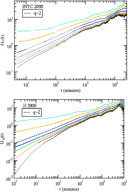
Figure 1: (Color online) Log–log plot of the generalized price–price correlation function $G_{q}(t)$ vs. $t$ corresponding to minute–to–minute INTC stock (top) and JJ stock (bottom) for $q=1/8,1/4,1/2,1,2,4,8$ from bottom to top in each panel.

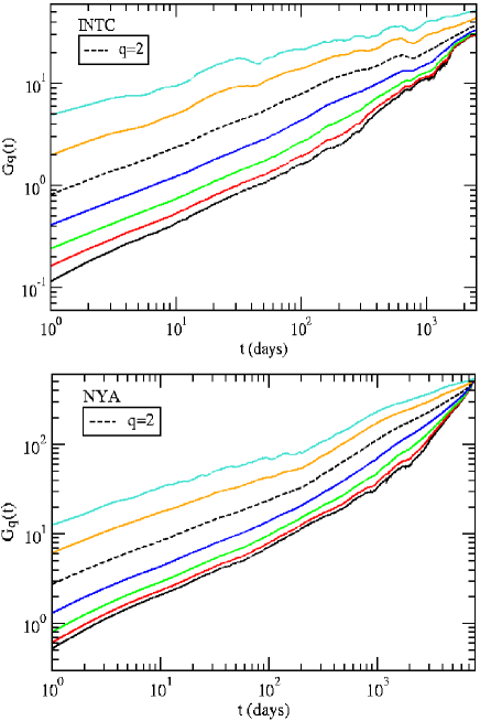
Figure 2: (Color online) Log–log plot of the generalized price–price correlation function $G_{q}(t)$ vs. $t$ corresponding to the daily INTC stock (top) and NYA index (bottom) for $q=1/8,1/4,1/2,1,2,4,8$ from bottom to top in each panel.

We first discuss the results concerning the price–price correlation functions calculated using Eq. (1). In Fig. 1 we present the results of $G_{q}(t)$ for the high frequency stocks and in Fig. 2 for the low frequency stocks. It is obvious that since the log–log plots of $G_{q}(t)$ vs. $t$ do not exhibit linear behavior over the entire time range the associated Hurst exponent $H_{q}$ varies with time and the scaling of the correlation functions suffers many transient regimes. A good power–law dependence appears for $q=2$. Although for other values of $q$ the deviations from power–law become visible it is clear that $H_{q}$ decreases with $q$. For illustration purpose we have fitted certain portions of these log–log plots to obtain a qualitative view of the dependence of $H_{q}$ on $1/q$, as shown in Fig. 3. In this figure we have used a large range of values for $q$ (i.e., $q=1/10,1/9,...,1,2,...,10$). We notice that $H_{q}$ depends linearly on $1/q$ for both small and large values of $1/q$. The stock with the smallest sampling time of $\delta t=1$ minute (JJ 2000) displays an increase of $H_{q}$ at large values of $1/q$, while for the rest of the stocks $H_{q}$ has the tendency to saturate as $1/q$ increases.

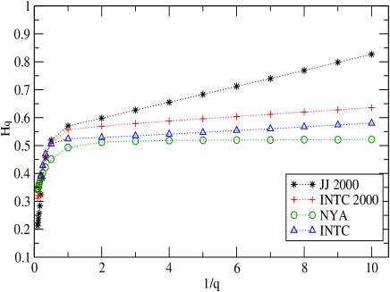
Figure 3: (Color online) The generalized Hurst exponent $H_{q}$ vs. $1/q$ for the four stocks discussed in the paper. $H_{q}$ behaves linearly with $1/q$ at both small and large values of $1/q$. For the daily stocks a linear least–square fit has been applied to the first two decades, while for the high frequency stocks, the fitted regions were $25<t<500$ for the INTC 2000 stock and $25<t<400$ for the JJ 2000 stock.

When using the MF-DFA method to calculate the correlation functions of order $q$ we note that the power–law behavior of $f_{q}(\tau)$ vs. $\tau$ extends over longer time periods making the extraction of the exponent $H_{q}$ more reliable. The results are shown in Figs. 4 and 5. This can be easily seen in the case of the daily NYA index and INTC stocks. The power–law is seen for more than three decades in Fig. 5, while limited power–laws spanning two decades only are seen in Fig. 2.

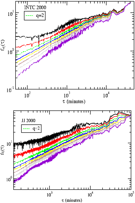
Figure 4: (Color online) Log–log plot of the normalized fluctuation function $f_{q}(\tau)$ vs. time lag $\tau$ corresponding to INTC 2000 stock (top) and JJ 2000 stock (bottom). The MF-DFA method has been used. The curves shown correspond to $q=-8,-4,-2,-1/2,1/2,2,4,8$ from bottom to top in each panel.

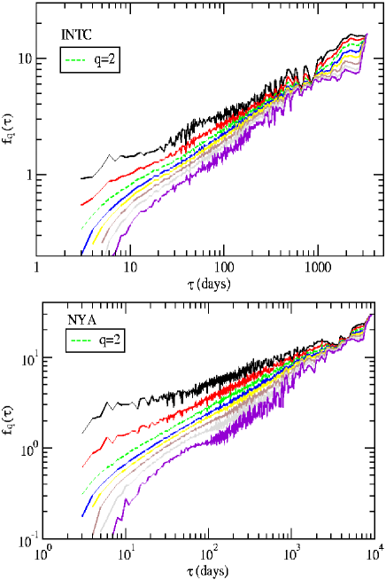
Figure 5: (Color online) Log–log plot of the normalized fluctuation function $f_{q}(\tau)$ vs. $\tau$ corresponding to the daily INTC stock (top) and NYA index (bottom). The MF-DFA method has been used to calculate $f_{q}(\tau)$. The curves shown correspond to $-8,-4,-2,-1/2,1/2,2,4,8$ from bottom to top in each panel.

As we have already mentioned, the value of $H_{q}$ is sensitive to the fitted region of the log–log plot of $f_{q}(\tau)$ vs. $\tau$. This issue requires special treatment. Our strategy was to take advantage of the analytic result of Eq. (19) in order to identify the time window over which the second order Hurst exponent can be extracted correctly. This can be achieved by adjusting $H_{2}$ such that the agreement between the empirical results for $f_{2}(\tau)$ using Eq. (17) and the theoretical curve predicted by Eq. (18) with $q=2$ and Eq. (19) becomes very good. This procedure is shown in Fig. 6. Once the time window which gives the best agreement for $q=2$ is identified, we use it to extract $H_{q}$ for a large set of $q$ values ($q=\pm 8,\pm 4,\pm 2,\pm 1,\pm 1/2,\pm 1/4,\pm 1/8$). The results for the $q$–dependence of $H_{q}$ based on the MF-DFA method have been used to calculate the multifractal spectra, $\tau_{q}=qH_{q}-1$, shown in Fig. 7. We observe that all spectra deviate from a linear $q$–dependence, which is an obvious manifestation of the multifractality in these stocks. In the inset of Fig. 7 we also show the $1/q$–dependence of $H_{q}$. At positive $q$, the qualitative trend of the results is the same as in Fig. 3. It is interesting to point out that the empirical set with the smallest sampling time, JJ 2000, which in the case of the standard price–price correlation function analysis has shown an increasing trend of $H_{q}$ at large values of $1/q$, does not present this trend anymore, $H_{q}$ saturating quickly as $1/q$ increases. Negative values of $q$ are accessible within the MF–DFA analysis. For large negative values of $1/q$ the generalized Hurst exponents saturate rather fast, as in the case of large positive values of $1/q$.

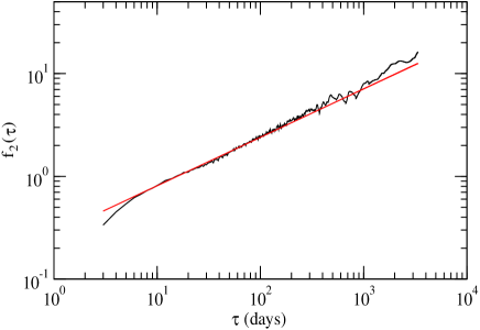
Figure 6: (Color online) The normalized fluctuation function $f_{2}(\tau)$ as a function of time for the daily INTC stock during the period 1990–2002. The straight line represents the theoretical curve based on Eqs. (18) and (19) for $H_{2}=0.47$.

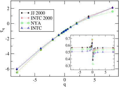
Figure 7: (Color online) The multifractal spectra $\tau_{q}$ vs. $q$ for the stocks discussed in the paper. The deviation of all curves from the linear dependence is a signature of the multifractal behavior. The inset shows the $1/q$–dependence of $H_{q}$, keeping the same symbol–stock correspondence as in the main figure.

The fact that $H_{q}$ (and in particular $H_{2}$) changes with time is a clear indication of the multifractal character. In this context we mention that the so–called multifractional Brownian motion could be alternatively used to model this feature Costa .

The analogy of the stock market fluctuations and fluid turbulence has already been pointed out in the literature turb_prev . It is known that in turbulent fluids the energy dissipation rate shows violent fluctuations. Similarly, as shown in Fig. 8, we find that the temporal evolution of the local stock price differences, $|x(t+\delta t)-x(t)|$, presents strong fluctuations which represent the signature of intermittency. In addition, the self-extending similarity features of intermittent fluid turbulence have been shown to exist in $spatial$ height correlation functions of the kinetic surface roughening models. We show in Figs. 8 and 9 that the extended self–similarity exhibited by the structure functions in fluid turbulence also shows up in the $temporal$ behavior of the financial stocks correlation functions. This observation offers a connection between three distinct physical problems, apparently without any intuitive connections: fluid turbulence, surface roughening and financial stocks.

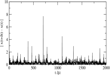
Figure 8: The local stock price difference $|x(t+\delta t)-x(t)|$ vs. the dimensionless variable $t/\delta t$ for the INTC 2000 recorded with sampling time $\delta t=5$ minutes.

For exemplification purpose we plot in Figs. 9 and 10 $\mbox{log}|f_{m}(\tau)|$ vs. $\mbox{log}|f_{n}(\tau)|$ for $m=-1/2$ and $2$ and $n=1$. From the linear behavior of these plots it is obvious that $f_{m}(\tau)\sim\left[f_{n}(\tau)\right]^{\alpha_{mn}}$, where the expectation value for the exponents $\alpha_{mn}$ is $\alpha_{mn}=H_{m}/H_{n}$. We find that our empirical results for $\alpha_{mn}$ are in very good agreement with the expected ratios between $H_{m}$ and $H_{n}$, as summarized in Table 1. It would be interesting to check the existence of the extended self–similarity in other financial stocks. We mention that the analysis of correlation functions based on the extended self–similarity is known to provide reliable values of the ratios between several generalized Hurst exponents Patcha .

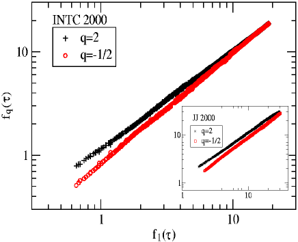
Figure 9: (Color online) The normalized fluctuation functions $f_{2}(\tau)$ and $f_{-1/2}(\tau)$ as a function of $f_{1}(\tau)$ for the INTC 2000 and JJ 2000 (inset) stocks.

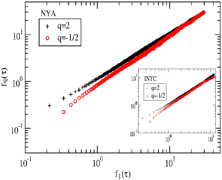
Figure 10: (Color online) The normalized fluctuation functions $f_{2}(\tau)$ and $f_{-1/2}(\tau)$ as a function of $f_{1}(\tau)$ for the daily NYA and INTC (inset) stocks.

Stock	$H_{2}/H_{1}$	$H_{-\frac{1}{2}}/H_{1}$	$\alpha_{2,1}$	$\alpha_{-\frac{1}{2},1}$
INTC	$0.966$	$1.051$	$0.956$	$1.065$
NYA	$0.960$	$1.059$	$0.961$	$1.058$
INTC 2000	$0.958$	$1.062$	$0.956$	$1.065$
JJ 2000	$0.983$	$1.033$	$0.962$	$1.040$

Table 1: Extended self-similar behavior of financial stocks based on the power–law dependence of $\mbox{log}|f_{m}(\tau)|$ on $\mbox{log}|f_{n}(\tau)|$ ($m=-\frac{1}{2}$ and $2$ and $n=1$). The exponents $\alpha_{-\frac{1}{2},1}$ and $\alpha_{2,1}$ extracted from the power–laws shown in Figs. 9 and 10 are in very good agreement with the expected ratios of $H_{-\frac{1}{2}}/H_{1}$ and $H_{2}/H_{1}$, respectively.

Next, we present in the results of the persistence probabilities and persistence exponents for our fluctuating stocks. In Fig. 11 we show the results based on the minute–to–minute stocks and in Fig. 12 the daily stocks. We observe that the best power–law appears for the average persistence probability $P(t)=1/2(P_{+}(t)+P_{-}(t))$, while departures from the power–law behavior can be seen for $P_{\pm}(t)$ corresponding to the INTC 2000 stock and more clearly for the daily stocks. For the low frequency stocks, in addition to measuring the positive, negative, and the average persistence probabilities of the stochastic price variables, we have also considered the set of these three probabilities corresponding to the empirical sets after the background elimination, i.e., $\tilde{x}(t)=x(t)-a\exp(bt)$. For the INTC stock we have that $a=1.1703$ and $b=1.1889\times 10^{-3}$, and for NYA index $a=28.473$ and $b=0.3177\times 10^{-3}$. The persistence curves for the variable $\tilde{x}(t)$ are very similar in the sense that no distinction between the positive, negative and average probabilities can be made. This result agrees with previous studies of the persistence probability of the German stock index Zheng . We have used $P(t)$ and $\widetilde{P}(t)$ in order to extract the persistence exponents for the minute–to–minute and daily stocks, respectively. The results are summarized in Tab. 2. We compared these values against $1-H_{2}$, with $H_{2}$ extracted from the fitted power–law of $f_{2}(\tau)$, in order to investigate the validity of Eq. (9). We find a good agreement between $\theta$ and $1-H_{2}$. However, it is important to emphasize that since both $\theta$ and $H_{2}$ are very close to $1/2$ the memory effects of the time series under investigation can only be revealed by higher order correlation functions. The second order correlation function by itself cannot explain the multifractality discussed in this study since it indicates that the returns are uncorrelated. We also add that $P(t)$ is not sensitive to the large discrepancy between $\delta t$ and $t_{m}$ corresponding to the high frequency stocks and daily stocks, respectively.

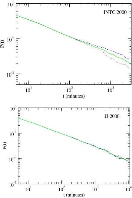
Figure 11: (Color online) Persistence probabilities $P(t)$ vs. $t$ for the minute–to–minute stocks. The dashed line corresponds to $P_{+}(t)$, the dotted line corresponds to $P_{-}(t)$, and the solid line represents $P(t)$.

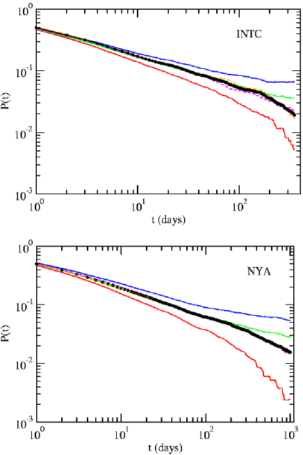
Figure 12: (Color online) Persistence probabilities $P(t)$ vs. $t$ for the daily stocks. Solid lines correspond to $P_{+}(t)$, $P(t)$, and $P_{-}(t)$ (from top to bottom). The dashed lines correspond to $\widetilde{P}_{+}(t)$ and $\widetilde{P}_{-}(t)$. The circle represents the average probability $\widetilde{P}(t)$ for the variable $\tilde{x}(t)$.

Stock	$\theta$	$H_{2}$
INTC	$0.51$	$0.47$
NYA	$0.50$	$0.50$
INTC 2000	$0.50$	$0.47$
JJ 2000	$0.52$	$0.47$

Table 2: The persistence exponent $\theta$ associated with the power–law decay of the average probability $P(t)$ ($\widetilde{P}(t)$) for the minute–to–minute stocks (daily stocks). $H_{2}$ is the second order Hurst exponent extracted from the time evolution of $f_{2}(\tau)$ (see Eq. (18)).

The generalization of the persistence probability is shown in Fig. 13. We only present the results for the probability of persistent large deviations corresponding to the INTC 2000 stock, but we have checked the applicability of this concept to other empirical stocks as well. From the linear behavior of $\mbox{log}P(t,s)$ vs. $\mbox{log}t$ we conclude that the $t$–dependence of $P(t,s)$ is indeed a power–law. We see that the local slope decreases as the average sign parameter $s$ decreases. We have varied $s$ from $-1$ to $1$ with an increment of $0.1$ and the $s$–dependence of the resulting family of persistent large deviations exponents is shown in the inset of Fig. 13. We mention that each curve in Fig. 13 corresponds to the average between the positive and negative persistent large deviations probabilities, i.e., $P(t,s)=1/2(P_{+}(t,s)+P_{-}(t,s))$. Both $P_{+}(t,s)$ and $P_{-}(t,s)$ show departures from the expected power–laws at large $t$, as we have seen in Figs. 11 and 12 in the case of the positive and negative persistence probabilities.

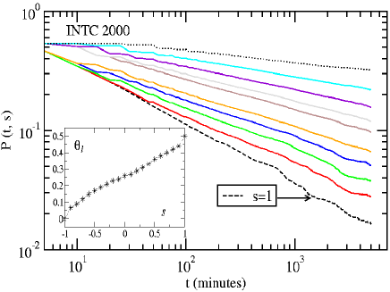
Figure 13: (Color online) Log–log plot of the persistent large deviations probability $P(t,s)$ vs. $t$ for the INTC 2000 stock. The average sign parameter, $s$, is varied from 1 to -0.8 (bottom to top) with an increment of 0.2. The inset contains the persistent large deviations exponent $\theta_{l}$ vs. $s$.

Finally we show the results of the survival probability in Fig. 14. We have looked at the temporal evolution of the JJ 2000 stock price recorded with two different sampling times, of 1 and 5 minutes, respectively. We have chosen different values of the measurement time, $t_{m}$, which influences directly the value of the average price $\bar{x}=1/t_{m}\int_{0}^{t_{m}}{dt^{\prime}~{}x(t^{\prime})}$. As shown in upper panel of Fig. 14 the survival probability measured over a longer $t_{m}$ has a slower decrease with time than the one corresponding to a smaller $t_{m}$. We find that the empirical measurements of $S(t)$ show good scaling with $t/\delta t$ at short times ($t<300$ minutes), when the ration between the sampling time and measurement time is kept constant. This agrees with similar measurements done on experimental step fluctuations dan_PRE . Since a very simple interpretation of the stock market fluctuations is based on the random walk model, we have numerically simulated the survival behavior of a random walker which allows us to understand qualitatively all the features of $S(t)$ found experimentally. Measurements of $S(t)$ for the random walk model were carried out for systems of size $L=100$. The measured average of the random walker variable at each site over the measurement time was used as the reference level in the calculation of the survival probability and the results were averaged over 300 independent runs. In bottom panel of Fig. 14 we show that a perfect collapse of $S(t)$ vs. $t/\delta t$ appears when the ratio $\delta t/t_{m}$ is constant. In addition, $S(t)$ corresponding to the data recorded with the same $\delta t$ shows a slower decrease when the measurement time is larger, as in the empirical case. Therefore both sampling time and total measurement time have to be taken into consideration in order to interpret correctly the survival features of the financial systems. We want to point out that $S(t)$ does not show an exponential behavior over the investigated time range (see the inset of the bottom panel of Fig. 14), and possibly much larger $t_{m}$ is needed to observe such a behavior at large time scales, as it happens in the case of equilibrium surface step fluctuations survival .

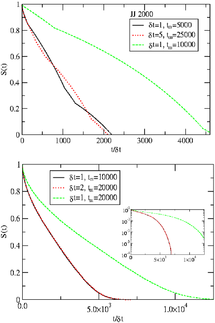
Figure 14: (Color online) The average survival probability $S(t)$ vs. $t/\delta t$ for the JJ 2000 stock (top) with different sampling times and different measurement times, as shown in the legend. The bottom plot contains the numerical simulation of $S(t)$ corresponding to a random walk with $L=100$. The scaling of $S(t)$ with $t/\delta t$ appears when $\delta t/t_{m}$ is constant. The inset shows the same curves on a logarithmic–linear scale.

IV Conclusions

We conclude with some speculative thoughts on the possible development of “understanding” in the sense of physics with respect to stock price fluctuations. In physics, e.g. step fluctuations krug ; magda1 ; magda_Pts ; dan_PRE ; survival or kinetic surface roughening barabasi , one typically looks for minimal (in the renormalization group sense) dynamical (in general, nonlinear) stochastic continuum partial differential equations underlying the stochastic phenomena, e.g., the Edwards–Wilkinson equation EW , the Mullins–Herring equation MH , the Kardar–Parisi–Zhang equation KPZ , the Villain–Lai–Das Sarma equation vill ; LD , etc., hoping to derive the long–time coarse–grained asymptotic power law behavior of the system arising from some simple minimal underlying dynamics (which is often based on symmetry and universality considerations). It is unclear whether such an approach based on continuum nonlinear stochastic equations is at all meaningful for the understanding of the dynamical evolution of complex economic phenomena such as stock price fluctuations. It may be possible to empirically construct dynamical equations which are sufficient to reproduce the exponents and the related statistical stochastic behavior described in this paper, but the necessary conditions for obtaining such equations are simply unknown (in fact, we do not know if such equations exist, except in some “trivial” data fitting sense). It is therefore quite intriguing that stock price fluctuation data are amenable to stochastic analyses based on first–passage statistics and multifractality (as carried out in this article) with results not that dissimilar from physical processes such as step fluctuations or nonequilibrium growth.

Our work demonstrates that the persistence and the multifractal behaviors of stock prices (both individual and composite) are subtle (including extended self-similar properties not identified in the literature before). It will be of interest to investigate if the empirical behavior we report in this paper can be derived from the various multifractal stochastic models Bacry:PRE ; Bacry:2001 ; Pochart:preprint ; Eisler:2004 for stock price fluctuations proposed in the literature. Such investigations, clearly beyond the scope of the current work, would, however, be quite difficult since both persistence and extended self–similarity are notoriously difficult concepts to derive theoretically, even when the underlying non–Markovian dynamics is known for a process. At this early stage of our understanding of econophysics, the fact that the stock price fluctuations seem to follow the persistence and the multifractal properties of well–studied surface fluctuation phenomena is by itself intriguing and interesting.

To summarize, in this study we have analyzed the multifractality, extended self–similarity, and first–passage properties of several financial stocks. While the second order Hurst exponent and the persistence exponent characterizing the power–law decay of the average persistence probability are not able to explain the long–term correlations in the investigated price time series, higher order correlation functions reveal much richer information about the complicated dynamics of such systems. We have shown that the persistence exponent $\theta$ is in agreement with $1-H_{2}$ and does not depend on the sampling time and measurement time. However, the survival probability has a nontrivial dependence on both $\delta t$ and $t_{m}$, presenting scaling with $t/\delta t$ only when the ration $\delta t/t_{m}$ is a constant. The numerical simulations of persistence, survival, and extended self–similarity features using discrete models of financial stocks remain on interesting open problem.

The authors wish to thank A. Christian Silva and Victor M. Yakovenko for useful discussions and providing most of the empirical data sets used in this study. We are indebted to Professor Michael E. Fisher for his proof reading of our manuscript and his positive comments. This work is partially supported by the NSF and U.S. ONR.

References

- (1) M. Ausloos and K. Ivanova, Comput. Phys. Commun. 147, 582 (2002).
- (2) N. Vandewalle, M. Ausloos, Eur. Phys. J. B 4, 257 (1998).
- (3) K. Matia, Y. Ashkenazy, H. E. Stanley, Europhys. Lett 61, 422 (2003).
- (4) P. Oswiecimka, J. Kwapien and S. Drozdz, Physica A 347, 626 (2005).
- (5) F. Schmitt, D. Schertzer, and S. Lovejoy, Int. J. Theor. Appl. Fin. 3, 361 (2000).
- (6) K. Kim and S.-M. Yoon, cond-mat/0305270
- (7) J. W. Lee, K. E. Lee, and P. A. Rikvold, arXiv:nlin.CD/0412038, to appear in Physica A.
- (8) B. Mandelbrot, A. Fisher, L. Calvet, A Multifractal Model of Asset Returns, Cowles Foundation Discussion Paper 1164 (1997) (unpublished).
- (9) T. Lux, The Multi-Fractal Model of Asset Returns: Its Estimation via GMM and Its Use for Volatility Forecasting, University of Kiel, Working Paper (2003) (unpublished).
- (10) E. Bacry, J. Delour and J. F. Muzy, Phys. Rev. E 64, 026103 (2001).
- (11) E. Bacry, J. Delour and J. F. Muzy, Physica A 299, 84 (2001).
- (12) J. -P. Bouchaud, M. Potters and M. Meyer, Eur. Phys. J. B 13, 595 (2000).
- (13) B. Pochart and J.-P. Bouchaud, Quantitative Finance 2, 303 (2002).
- (14) Z. Eisler and J. Kertésza, Physica A, 343, 603 (2004).
- (15) J. Krug, H. Kallabis, S. N. Majumdar, S. J. Cornell, A. J. Bray and C. Sire, Phys. Rev. E 56, 2702 (1997).
- (16) M. Constantin, C. Dasgupta, P. Punyindu Chatraphorn, S. N. Majumdar, and S. Das Sarma, Phys. Rev. E 69, 061608 (2004).
- (17) B. Zheng, Mod. Phys. Lett. B 21, 775 (2002).
- (18) I. Simonsen, M. H. Jensen, and A. Johansen, Eur. Phys. J. B 27, 583 (2002).
- (19) A. -L. Barabasi and H. E. Stanley, Fractal Concepts in Surface Growth (Cambridge University Press, New York, 1995).
- (20) R. Benzi et al., Phys. Rev. E 48, R29 (1993).
- (21) G. Stolovitzky and K. R. Sreenivasan, Phys. Rev. E 48, R33 (1993) .
- (22) A. Kundagrami, C. Dasgupta, P. Punyindu and S. Das Sarma, Phys. Rev. E 57, R3703 (1998).
- (23) M. Constantin, S. Das Sarma, C. Dasgupta, O. Bondarchuk, D. B. Dougherty and E. D. Williams, Phys. Rev. Lett. 91, 086103 (2003).
- (24) D. B. Dougherty, C. Tao, O. Bondarchuk, W. G. Cullen, E. D. Williams, M. Constantin, C. Dasgupta, and S. Das Sarma, Phys. Rev. E 71, 021602 (2005).
- (25) C. Dasgupta, M. Constantin, S. Das Sarma, and Satya N. Majumdar, Phys. Rev. E 69, 022101 (2004).
- (26) J. Krug, Adv. Phys. 46, 139 (1997).
- (27) J. W. Kantelhardt, S. A. Zschiegner, E. Koscielny-Bunde, A. Bunde, S. Havlin, H. E. Stanley, Physica A 316, 87 (2002).
- (28) C.-K. Peng et al., Phys. Rev. E 49 1685 (1994).
- (29) A. Christian Silva, Richard E. Prange, and Victor M. Yakovenko, Physica A 344, 227 (2004).
- (30) N. Vandevalle, Ph. Boveroux, A. Minguet, and M. Ausloos, Physics A 255, 201 (1998).
- (31) B. B. Mandelbrot and J.W. van Ness, SIAM Rev. 10, 422 (1968).
- (32) S. M. Berman, Ann. Math. Stat. 41, 1260 (1970).
- (33) A. Hansen, T. Engoy and K. J. Maloy, Fractals 2, 527 (1994).
- (34) M. Ding and W. Yang, Phys. Rev. E 52, 207 (1995).
- (35) S. Maslov, M. Paczuski and P. Bak, Phys. Rev. Lett. 73, 2162 (1994).
- (36) I. Dornic and C. Godreche, J. Phys. A: Math. Gen. 31, 5413 (1998).
- (37) J. Feder, Fractals, Plenum Press, New York, 1988.
- (38) R. L. Costa and G. L. Vasconcelos, Physica A 329, 231 (2003).
- (39) M. S. Taqqu, V. Teverovsky, W. Willinger, Fractals 3, 785 (1995).
- (40) R. N. Mantegna and H. E. Stanley, Nature 383, 587 (1996).
- (41) S. F. Edwards and D. R. Wilkinson, Proc. R. Socs. London, Ser.A 381, 17 (1982).
- (42) W. W. Mullins, J. Appl. Phys. 28, 333 (1957); C. Herring, J. Appl. Phys. 21, 301 (1950).
- (43) M. Kardar, G. Parisi, and Y. -C. Zhang, Phys. Rev. Lett. 56, 889 (1986).
- (44) J. Villain, J. Phys. I (France) 1, 19 (1991).
- (45) Z. -W. Lai and S. Das Sarma, Phys. Rev. Lett. 66, 2348 (1991).