Two Models for Bolometer and Microcalorimeter Detectors with Complex Thermal Architectures

Abstract

We have developed two analytical models to describe the performance of cryogenic microcalorimeters and bolometers. One of the models is suitable to describe Transition Edge Sensor(TES) detectors with an integrated absorber, the other is suitable for detectors with large absorbers. Both models take into account hot-electron decoupling and absorber decoupling. The differential equations describing these models have been solved using block diagram algebra. Each model has produced closed form solutions for the detector’s responsivity, dynamic impedance, and noise equivalent power for phonon noise, Johnson noise, amplifier noise, 1/f noise, and load resistor noise.

1 Introduction

The operational principle of simple microcalorimeters and bolometers is based on three components. An absorber where the incoming power or energy is dissipated and converted into a change in temperature, a sensor that reads the change in temperature, and a thermal link from the detector to the heat sink that brings the system back to equilibrium after a measurement. The sensor is usually a resistor whose resistance depends strongly on temperature around the working point. In this case a change in resistance can be measured as a change in voltage or a change in current using a current or voltage bias.

In 1982 J.C Mather [1] presented a complete non-equilibrium theory for the noise in simple bolometers with ideal resistive thermometers and in 1984 it was extended to microcalorimeter performance [2]. At temperatures below  200 mK the ideal assumptions are no longer valid and complex thermal architectures are needed to understand the behavior of these devices. At these low temperatures the thermal fluctuations between the thermometer lattice and its electron system, or between the thermometer and the absorber are no longer negligible and therefore these components must be considered as separate entities in the model. These non-ideal effects are called electron decoupling and absorber decoupling. Another consequence of working at low temperatures is the increased dependence of the thermometer resistance on the readout power, making the ideal resistance-temperature relationship inaccurate. Galeazzi and McCammon [3] constructed a general procedure for developing bolometer and microcalorimeter models for these complex thermal architectures using block diagram formalism of control theory.

To quantify the relation between incoming power or energy and the measured change in voltage or current, including non-ideal effects, this paper follows the modeling procedure of Galeazzi and McCammon [3]. The first step in this modeling procedure is to set up the temperature equations, then apply a Taylor expansion to derive a linear model for small temperature deviations from equilibrium. Afterward, Fourier transforms are used to express the equations in the frequency domain, and finally the coupled equations are solved using block diagram algebra. This procedure yields closed form solutions for the responsivity and dynamic impedance of the model, including noise contributions.

The two models developed in this paper are modifications of the absorber decoupling model obtained in [3]. Model 1 was developed to describe the new generation of transition edge sensor detectors where the absorber is not electrically isolated from the thermometer by a gluing agent but rather the two are deposited one on top of the other [4]. Model 2 describes microcalorimeters that have the heat sink connected to the absorber instead of to the thermometer. This may occur when the absorber is much bigger than the thermometer and therefore it is necessary to connect the heat sink to the absorber rather than to the thermometer. These two models will help optimize the next generation of detectors, and because of the analytical results of the modeling procedure the relations between the detector’s resolution and the different parameters included in the model should be clear.

2 Model 1

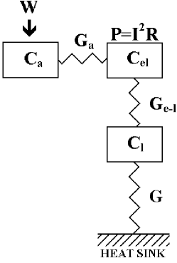
Figure 1: Thermal architecture of Model 1.

This model is suitable to describe TES detectors with an integrated absorber. In this model both the electron system and the absorber are detached from the lattice. The lattice is connected to the heat sink by a thermal conductivity $G$, the electron system is connected to the lattice by a thermal conductivity $G_{e-l}$, and the absorber is connected to the electron system by a thermal conductivity $G_{a}$ ( see Fig. 1). The absorber is directly connected to the electron system instead of the lattice because with integrated absorbers the absorber-lattice thermal coupling is expected to be negligible compared to that of the absorber-electron system.

2.1 Responsivity S($\omega$)

The following equations determine the temperature for each of the three components in the model:

$$C_{a}\frac{d(T^{\prime}_{a})}{dt}+\int_{T^{\prime}_{e}}^{T^{\prime}_{a}}G_{a}(T^{\prime})dT^{\prime}=W$$ (1)

$$C_{e}\frac{d(T^{\prime}_{e})}{dt}+\int_{T^{\prime}_{a}}^{T^{\prime}_{e}}G_{a}(T^{\prime})dT^{\prime}+\int_{T^{\prime}_{l}}^{T^{\prime}_{e}}G_{e-l}(T^{\prime})dT^{\prime}=P(T^{\prime}_{e})$$ (2)

$$C_{l}\frac{d(T^{\prime}_{l})}{dt}+\int_{T^{\prime}_{e}}^{T^{\prime}_{l}}G_{e-l}(T^{\prime})dT^{\prime}+\int_{T_{s}}^{T^{\prime}_{l}}G(T^{\prime})dT^{\prime}=0,$$ (3)

where $C_{a}$, $C_{e}$, and $C_{l}$ are the heat capacities of the absorber, the electron system, and the lattice system respectively, and $T^{\prime}_{a}$, $T^{\prime}_{e}$, and $T^{\prime}_{l}$ are the corresponding temperatures. $W$ is the incoming outside power to be measured and $P(T^{\prime}_{e})$ is the Joule power dissipated into the sensor by the bias current/voltage. In the case of microcalorimeters $W=E\delta(t_{o})$, where $E$ is the photon energy and $\delta(t_{o})$ is the delta function.

The equilibrium conditions of the system are obtained by setting the outside power to zero ($W=0$), and $d(T^{\prime}_{x})/dt=0$ ($x$= $a$, $e$, or $l$) since the equilibrium temperatures are independent of time. Therefore the equilibrium temperatures $T_{a}$ of the absorber, $T_{e}$ of the electron system, and $T_{l}$ of the lattice are given by the integrals in the previous three equations. For example the integral in Eq. 1 must equal zero at equilibrium, which implies that the thermal equilibrium temperature of the absorber is the same as that of the electron system. We are interested in small deviations about the equilibrium temperatures, therefore we set $T^{\prime}_{x}=T_{x}+\Delta T_{x}$, where $T_{x}$ is the equilibrium temperature for each component of the model, and $\Delta T_{x}$ is the small temperature deviation from equilibrium:

$$C_{a}\frac{d(T_{a}+\Delta T_{a})}{dt}+\int_{T_{e}+\Delta T_{e}}^{T_{a}+\Delta T_{a}}G_{a}(T^{\prime})dT^{\prime}=W$$ (4)

$$C_{e}\frac{d(T_{e}+\Delta T_{e})}{dt}+\int_{T_{a}+\Delta T_{a}}^{T_{e}+\Delta T_{e}}G_{a}(T^{\prime})dT^{\prime}+\int_{T_{l}+\Delta T_{l}}^{T_{e}+\Delta T_{e}}G_{e-l}(T^{\prime})dT^{\prime}=P(T_{e}+\Delta T_{e})$$ (5)

$$C_{l}\frac{d(T_{l}+\Delta T_{l})}{dt}+\int_{T_{e}+\Delta T_{e}}^{T_{l}+\Delta T_{l}}G_{e-l}(T^{\prime})dT^{\prime}+\int_{T_{s}}^{T_{l}+\Delta T_{l}}G(T^{\prime})dT^{\prime}=0.$$ (6)

In the small signal limit $\Delta T_{x}$ is small compared to $T_{x}$, and a Taylor expansion up to the first $\Delta T_{x}$ term is appropriate. The results are the equations that determine small temperature deviations about equilibrium:

$$C_{a}\frac{d(\Delta{T_{a}})}{dt}+G_{a}\Delta T_{a}=W+G_{a}\Delta T_{e}$$ (7)

$$C_{e}\frac{d(\Delta{T_{e}})}{dt}+G_{a}\Delta T_{e}+G_{e-l}(T_{e})\Delta T_{e}=\Delta P+G_{a}\Delta T_{a}+G_{e-l}(T_{l})\Delta T_{l}$$ (8)

$$C_{l}\frac{d(\Delta T_{l})}{dt}+G_{e-l}(T_{l})\Delta T_{l}+G\Delta T_{l}=G_{e-l}(T_{e})\Delta T_{e},$$ (9)

where $\Delta P=P(T_{e}+\Delta T_{e})-P(T_{e})$, and for simplicity we used $G_{a}=G_{a}(T_{a})$ and $G=G(T_{l})$.

These are coupled differential equations which are difficult to solve directly; instead they are transformed into coupled algebraic equations using Fourier transforms. The quantity $\Delta P$ represents what is known as the electro-thermal feedback term and can be written as $\Delta P=-G_{ETF}\Delta T_{e}$, where $G_{ETF}=P(R-R_{L})\alpha/T_{e}R(R_{L}+R)$; (see reference [3]). Converting Eqs. 7, 8, and 9 into the frequency domain using Fourier transforms we obtain:

$$j\omega C_{a}\Delta T_{a}+G_{a}\Delta T_{a}=W+G_{a}\Delta T_{e}$$ (10)

$$j\omega C_{e}\Delta T_{e}+(G_{a}+G_{e-l}(T_{e})+G_{ETF})\Delta T_{e}=G_{a}\Delta T_{a}+G_{e-l}(T_{l})\Delta T_{l}$$ (11)

$$j\omega C_{l}\Delta T_{l}+(G_{e-l}(T_{l})+G)\Delta T_{l}=G_{e-l}(T_{e})\Delta T_{e}.$$ (12)

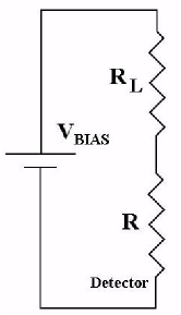
Figure 2: Typical readout circuit. Notice that if $R_{L}<<R$ the detector is voltage biased, if $R_{L}>>R$ the detector is current biased.

With these equations it is possible to solve for $\Delta T_{e}$, which can be related to the measured quantities $\Delta I$ or $\Delta V$, using the typical detector readout circuit of Fig. 2:

$$\Delta V=V\frac{\alpha}{T_{e}}\frac{R_{L}}{R_{L}+R}\Delta T_{e}$$ (13)

$$\Delta I=-I\frac{\alpha}{T_{e}}\frac{R}{R_{L}+R}\Delta T_{e},$$ (14)

where $\alpha=T_{e}/R\times dR/dT_{e}$ is the sensitivity of the detector, $R_{L}$ is the load resistance, $R$ is the resistance of the detector, $V$ is the voltage across $R$, and $I$ is the current flowing through $R$.

To simplify the notation let $X$ be either $V$ or $I$, and introduce the quantity $A_{tr}=R/X\times dX/dR$ to be deduced from the previous two equations. Then Eqs. 13 and 14 can be summarized as:

$$\frac{\Delta X}{X}=\alpha A_{tr}\frac{\Delta T_{e}}{T_{e}}.$$ (15)

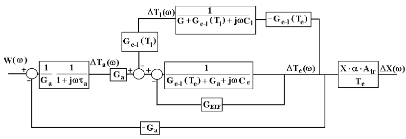
Figure 3: Block diagram representing Model 1.

Equations 10, 11, 12, and 15 can be solved using the block diagram of Fig. 3. To set up the block diagram consider the left hand side of Eqs.10, 11, 12, and 15 as the response function of the absorber system, electron system, lattice system, and circuit readout respectively. The right hand side of these equations corresponds to the input to each system. Connecting the response functions with their appropriate inputs leads to the block diagram of Fig. 3.

To solve the block diagram in Fig. 3 for $\Delta X(\omega)$ we used the procedure and simplification rules of the block diagram formalism described in [3]. This result is then used to find the responsivity, which is defined as $S(\omega)=\Delta X(\omega)/W(\omega)$. The following responsivity characterizes the response of Model 1 detectors:

$$S(w)=\frac{G_{a}}{(G_{a}+j\omega C_{a})\bigg{[}(G_{a}+G_{e-l}(T_{e})+G_{ETF}+j\omega C_{e})-\frac{G_{e-l}(T_{l})G_{e-l}(T_{e})}{j\omega C+G_{e-l}(T_{l})+G}\bigg{]}-G_{a}^{2}}\frac{X\alpha A_{tr}}{T_{e}}.$$ (16)

2.2 Dynamic Impedance

A detector can also be described by its complex dynamic impedance $Z(\omega)=dV(\omega)/dI(\omega)$. The dynamic impedance differs from the detector resistance due to the effect of the electro-thermal feedback. When the current changes, the power dissipated into the detector changes too, therefore the temperature and the detector’s resistance change. The dynamic impedance is a useful parameter because it is easily measured experimentally. To find the dynamic impedance we use $-G_{ETF}\Delta T_{e}=\Delta P$ in Eqs. 11, and use Eqs. 10, 11, and 12 to find $\Delta T_{e}$ in terms of $\Delta P$, $\omega$, the heat capacity of each of the three components, and the three thermal conductivities:

$$dT_{e}=\frac{dP}{\bigg{(}j\omega C_{e}+G_{a}+G_{e-l}(T_{e})-\frac{G_{a}^{2}}{G_{a}+j\omega C_{a}}-\frac{G_{e-l}(T_{l})G_{e-l}(T_{e})}{j\omega C+G_{e-l}(T_{l})+G}\bigg{)}}.$$ (17)

Differentiating Ohm’s law ($V=IR$) and using the definition of sensitivity $\alpha$ we obtain:

$$dV=RdI+I\frac{\alpha RdT}{T}.$$ (18)

Substituting Eq. 17 into Eq 18 and using the fact that $dP=VdI+IdV$, it is possible to solve for $dV/dI$ and obtain the following result for the dynamic impedance:

$$Z(\omega)=\frac{dV}{dI}=R\frac{\bigg{[}\alpha P+T\bigg{(}j\omega C_{e}+G_{a}+G_{e-l}(T_{e})-\frac{G_{a}^{2}}{G_{a}+j\omega C_{a}}-\frac{G_{e-l}(T_{l})G_{e-l}(T_{e})}{j\omega C+G_{e-l}(T_{l})+G}\bigg{)}\bigg{]}}{\bigg{[}-\alpha P+T\bigg{(}j\omega C_{e}+G_{a}+G_{e-l}(T_{e})-\frac{G_{a}^{2}}{G_{a}+j\omega C_{a}}-\frac{G_{e-l}(T_{l})G_{e-l}(T_{e})}{j\omega C+G_{e-l}(T_{l})+G}\bigg{)}\bigg{]}}.$$ (19)

2.3 Noise

The effect of noise on a detector’s performance is quantified by the Noise Equivalent Power (NEP). It corresponds to the power that would be required as input to the detector in order to generate an output equal to the signal generated by the noise. The NEP can therefore be calculated as the ratio between the output generated by the noise and the responsivity of the detector:

$$NEP_{y}=\frac{\Delta X_{y}}{S(\omega)}.$$ (20)

The variable $y$ stands in for any of the possible noise terms: $amp$=amplifier noise, $j$=Johnson noise, $R_{L}$=load resistor noise, $1/f$=$1/f$ noise, $a$=absorber-electron system thermal noise, $th$=heat sink-lattice thermal noise or $he$=electron system-lattice thermal noise.

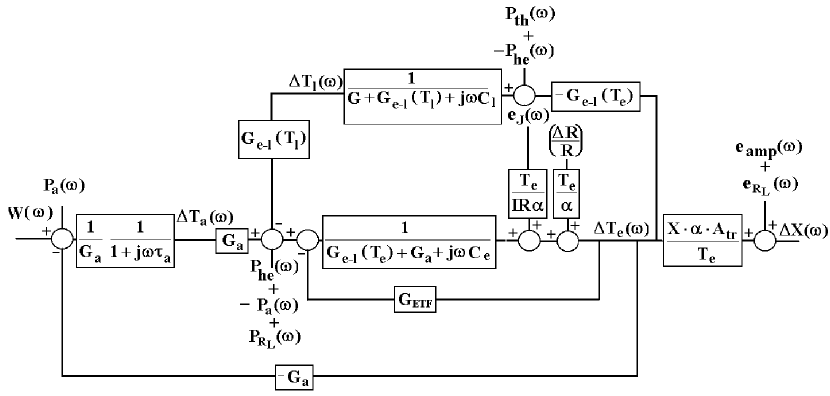
Figure 4: Block diagram including noise contributions for Model 1.

To obtain the Noise Equivalent Power for each term, the noise contributions $e_{amp}$, $e_{j}$, $e_{R_{L}}$, $P_{R_{L}}$, $(\Delta R/R)_{1/f}$, $P_{a}$, $P_{th}$, and $P_{he}$ must be added to the block diagram of Fig. 3. Figure 4 shows where each noise term should be added to the block diagram (for more details see [3]). Solving the noise block diagram for each noise term independently and dividing by the responsivity obtained in Eq. 16 we obtain the following NEP’s:

$$NEP_{a}=P_{a}(\omega)j\omega\tau_{a}$$ (21)

$$NEP_{R_{L}}=P_{R_{L}}(\omega)(1+j\omega\tau_{a})+\frac{e_{R_{L}}}{S(\omega)}$$ (22)

$$NEP_{amp}=\frac{e_{amp}}{S(\omega)}$$ (23)

$$NEP_{he}=P_{he}\frac{(1+j\omega\tau_{a})(G+j\omega C_{l})}{(G+G_{e-l}(T_{l})+j\omega C_{l})}$$ (24)

$$NEP_{th}=P_{th}\frac{G_{e-l}(T_{l})(1+j\omega\tau_{a})}{(G+G_{e-l}(T_{l})+j\omega C_{l})}$$ (25)

$$NEP_{e_{j}}=e_{j}(\omega)\frac{T_{e}}{IR\alpha}(1+j\omega\tau_{a})\bigg{(}G_{a}+G_{e-l}(T_{e})+j\omega C_{e}-$$

$$\frac{G_{e-l}(T_{l})G_{e-l}(T_{e})}{j\omega C+G_{e-l}(T_{l})+G}-\frac{G_{a}^{2}}{G_{a}+j\omega C_{a}}\bigg{)}$$ (26)

$$NEP_{1/f}=\Big{(}\frac{\Delta R(\omega)}{R}\Big{)}_{1/f}\frac{T_{e}}{\alpha}(1+j\omega\tau_{a})\bigg{(}G_{a}+G_{e-l}(T_{e})+j\omega C_{e}-$$

$$\frac{G_{e-l}(T_{l})G_{e-l}(T_{e})}{j\omega C+G_{e-l}(T_{l})+G}-\frac{G_{a}^{2}}{G_{a}+j\omega C_{a}}\bigg{)}.$$ (27)

Where $\tau_{a}=C_{a}/G_{a}$.

3 Model 2

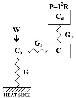
Figure 5: Thermal architecture of Model 2.

In experiments involving dark matter detectors and double-beta decay detectors the absorber size is significant and can have a mass up to almost 1 Kg [5]. For mechanical reasons these large absorbers must be mechanically connected to the heat sink. The thermal link between the detector and the heat sink can therefore also be through the absorber rather than through the sensor. Model 2 reflects this condition by having the absorber connected to the heat sink through a thermal conductivity $G$. Model 2 also takes into account absorber decoupling and electron decoupling by connecting the lattice system to the absorber through a thermal conductivity $G_{a}$ and by having the electron system connected to the lattice system through a thermal conductivity $G_{e-l}$ (see Fig. 5).

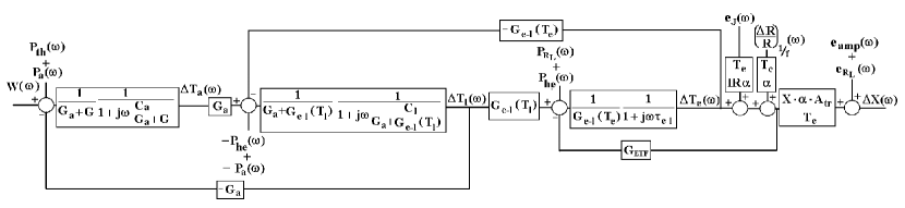
Figure 6: Block diagram including noise contributions for Model 2.

Applying the same procedure previously used for Model 1 we obtain for Model 2 the block diagram of Fig. 6.Solving the block diagram for the responsivity, the dynamic impedance, and all the noise contributions, we obtain the following results:

$$\scriptstyle S(\omega)=\frac{G_{a}G_{e-l}(T_{l})}{(G_{e-l}(T_{e})+G_{ETF}+j\omega C_{e})\bigg{[}(G_{a}+G_{e-l}(T_{l})+j\omega C_{l})(G_{a}+G+j\omega C_{a})-G_{a}^{2}\bigg{]}-G_{e-l}(T_{l})G_{e-l}(T_{e})(G_{a}+G+j\omega C_{a})}\frac{X\alpha A_{tr}}{T_{e}}$$ (28)

$$Z(\omega)=R\frac{\alpha P+T_{e}\bigg{[}j\omega C_{e}+G_{e-l}(T_{e})-G_{e-l}(T_{l})\bigg{(}\frac{G_{e-l}(T_{e})(j\omega C_{a}+G_{a}+G)}{(j\omega C_{a}+G_{a}+G)(j\omega C_{l}+G_{a}+G_{e-l}(T_{l}))-G_{a}^{2}}\bigg{)}\bigg{]}}{-\alpha P+T_{e}\bigg{[}j\omega C_{e}+G_{e-l}(T_{e})-G_{e-l}(T_{l})\bigg{(}\frac{G_{e-l}(T_{e})(j\omega C_{a}+G_{a}+G)}{(j\omega C_{a}+G_{a}+G)(j\omega C_{l}+G_{a}+G_{e-l}(T_{l}))-G_{a}^{2}}\bigg{)}\bigg{]}}$$ (29)

$$NEP_{th}=P_{th}$$ (30)

$$NEP_{amp}=\frac{e_{amp}}{S(\omega)}$$ (31)

$$NEP_{a}=P_{a}\bigg{[}\frac{G+j\omega C_{a}}{G_{a}}\bigg{]}$$ (32)

$$NEP_{he}=P_{he}\bigg{[}\frac{(G_{a}+G+j\omega C_{a})(G_{a}+G_{e-l}(T_{l})+j\omega C_{l})-G_{a}^{2}}{G_{a}G_{e-l}(T_{l})}-\frac{G+G_{a}+j\omega C_{a}}{G_{a}}\bigg{]}$$ (33)

$$NEP_{R_{L}}=P_{R_{L}}\bigg{[}\frac{(G_{a}+G+j\omega C_{a})(G_{a}+G_{e-l}(T_{l})+j\omega C_{l})-G_{a}^{2}}{G_{a}G_{e-l}(T_{l})}\bigg{]}+\frac{e_{RL}}{S(\omega)}$$ (34)

$$NEP_{e_{j}}=e_{j}\frac{T_{e}}{IR\alpha}\frac{(G_{a}+G+j\omega C_{a})[(G_{a}+G_{e-l}(T_{l})+j\omega C_{l})-\frac{G_{e-l}(T_{l})G_{e-l}(T_{e})}{j\omega C_{e}+G_{e-l}(T_{e})}]-G_{a}^{2}}{G_{a}G_{e-l}(T_{l})}$$

$$\times(j\omega C_{e}+G_{e-l})$$ (35)

$$NEP_{\frac{1}{f}}=\Big{(}\frac{\Delta R(\omega)}{R}\Big{)}_{\frac{1}{f}}\frac{(G_{a}+G+j\omega C_{a})[(G_{a}+G_{e-l}(T_{l})+j\omega C_{l})-\frac{G_{e-l}(T_{l})G_{e-l}(T_{e})}{j\omega C_{e}+G_{e-l}(T_{e})}]-G_{a}^{2}}{G_{a}G_{e-l}(T_{l})}$$

$$\times\frac{T_{e}}{\alpha}(j\omega C_{e}+G_{e-l}).$$ (36)

4 Examples of Energy Resolution and Time constant Results from the Models

In experimental setups of detectors some of the parameters are fixed while others can vary. With the freedom to vary a few parameters the goal is to optimize the detectors characteristics. The equations derived in this paper offer the flexibility and power to perform such operations. An example of such applications is reported in fig. 7. The characteristics of interest are energy resolution and the time constant of the detector. The energy resolution is calculated following equation 69 in reference [3]. The time constant is calculated as the inverse of the first turn frequency of the responsivity. The variable parameters in the examples of fig. 7 are: heat capacity of the absorber ($C_{a}$) vs. thermal conductivity between absorber and thermometer ($G_{a}$) and thermal conductivity between detector and heat sink ($G$) vs. thermal conductivity between absorber and thermometer ($G_{a}$). The fixed parameters are reported in Table 1. By inputing the fixed parameter into the two models of this paper and the model found in [3] and letting $C_{a}$, $G$ , and $G_{a}$ vary we obtain the twelve contour plots in fig. 7. The first six plots predict energy resolution while the last six plots refer to the detectors time constant. Each column of contour plots belongs to one of the three different models.

5 Conclusions

To improve the performance of microcalorimeters and bolometers it is important to accurately understand how this depends on the fabrications parameters. Significant improvements in detectors performance have, in fact, been achieved by optimizing the design based on an accurate model of the detector [6]. In this paper we derived detailed theoretical models to describe the behavior of two different detector architectures. The use of block diagram algebra has allowed us to present the results in an analytical form that can be easily and immediately utilized by investigators to improve the design of their detectors. Furthermore, the contour plots in fig. 7 provide an example of how the equations derived in this paper can be utilized to predict the characteristics of detectors.

Tables

Table 1: Values of the fixed parameters needed to produce the contour plots of fig. 7

Figures

FIG. 1: Thermal architecture of Model 1.

FIG. 2: Typical readout circuit. Notice that if $R_{L}<<R$ the detector is voltage biased, if $R_{L}>>R$ the detector is current biased.

FIG. 3: Block diagram representing Model 1.

FIG. 4: Block diagram including noise contributions for Model 1.

FIG. 5: Thermal architecture of Model 2.

FIG. 6: Block diagram including noise contributions for Model 2.

FIG. 7: Contour plots of how the energy resolution and time constant of each model change with respect to the heat capacity $C_{a}$ and the thermal conductivities $G$ and $G_{a}$. These plots were constructed using the fixed parameters in Table 1.

Table 1: Values of the fixed parameters needed to produce the contour plots in fig 7

Parameter	Value
$R$	$5m\Omega$
$R_{L}$	$0.2m\Omega$
$V_{bias}$	$1.0848\times 10^{-7}V$
$\alpha$	$100$
$C_{a}$	$1pJ/K$
$C_{l}$	$4.911\times 10^{-5}pJ/K$
$C_{e}$	$0.154pJ/K$
$T_{s}$	$0.1K$
$G_{e-l}(T_{l})$	$5\times 10^{-10}W/K$
$G_{e-l}(T_{e})$	$5.87\times 10^{-10}W/K$
$G$	$1\times 10^{-10}W/K$

Figure 7: Contour plots of how the energy resolution and time constant of each model change with respect to the heat capacity $C_{a}$ and the thermal conductivities $G$ and $G_{a}$. These plots were constructed using the fixed parameters in Table 1.