Activation entropy of electron transfer reactions

Abstract

We report microscopic calculations of free energies and entropies for intramolecular electron transfer reactions. The calculation algorithm combines the atomistic geometry and charge distribution of a molecular solute obtained from quantum calculations with the microscopic polarization response of a polar solvent expressed in terms of its polarization structure factors. The procedure is tested on a donor-acceptor complex in which ruthenium donor and cobalt acceptor sites are linked by a four-proline polypeptide. The reorganization energies and reaction energy gaps are calculated as a function of temperature by using structure factors obtained from our analytical procedure and from computer simulations. Good agreement between two procedures and with direct computer simulations of the reorganization energy is achieved. The microscopic algorithm is compared to the dielectric continuum calculations. We found that the strong dependence of the reorganization energy on the solvent refractive index predicted by continuum models is not supported by the microscopic theory. Also, the reorganization and overall solvation entropies are substantially larger in the microscopic theory compared to continuum models.

I Introduction

Beginning with work of Marcus on electron transfer (ET) between ions dissolved in polar solvents Marcus (1993), the understanding of the dynamics and thermodynamics of the nuclear polarization coupled to the transferred electron has been viewed as a key component of ET theories. The concept of polarization fluctuations as a major mechanism driving ET has been extended over the several decades of research from simple molecular solvents to a diversity of condensed-phase media of varying complexity. A significant part of the present experimental and theoretical effort is directed toward the understanding of ET in biology, where this process is a key component of energy transport chains Marcus and Sutin (1985); Winkler and Gray (1992); McLendon and Hake (1992); Warshel (2002). Biological systems pose a major challenge to theoretical and computational chemistry from at least two viewpoints. First, the solvent, including bulk and bound water Gregory (1995), membranes, and parts of the polar and polarizable matrix of the biopolymer, is highly anisotropic and heterogeneous. Second, the geometry of what can be separated as a solute is often very complex, including concave regions of molecular scale occupied by the solvent and regions of the biopolymer with a significant mobility of polar and ionizable residues.

Dielectric continuum models accommodate the complex solute shape by numerical algorithms solving the Poisson equation with the boundary conditions defined by a dielectric cavity Rocchia et al. (2001). The heterogeneous nature of the solvent in the vicinity of a redox site can in principle be included by assigning different dielectric constants to its heterogeneous parts Siriwong et al. (2003). Two fundamental problems inevitably arise in this algorithm. The first has been well recognized over the years of its application and is related to the ambiguity of defining the dielectric cavity for molecular solutes. This problem is often resolved by proper parameterization of the radii of atomic and molecular groups of the solute. The second problem is much less studied. It is related to the fact that collective polarization fluctuations of molecular dielectrics possess a finite correlation length which may be comparable to the length of concave regions of the solute or some other characteristic dimensions significant for solvation thermodynamics. The definition of the dielectric constant for polar regions of molecular length is very ambiguous and, in addition, once the dielectric constant is defined, it is not clear if the dielectric response can fully develop on the molecular length scale.

In addition to the problems in implementing the continuum formalism for molecular solutes there are some fundamental limitations of the continuum approximation itself that may limit its applicability to solvation and electron transfer thermodynamics. On the basic level, the definition of the molecular cavity should be re-done for each particular thermodynamic state of the solvent Roux et al. (1990); Lynden-Bell (1999) and/or electronic state of the solute Rick and Berne (1994). This precludes the use of continuum theories with a given cavity parametrization to describe derivatives of the solvation free energy, e.g. entropy and volume of solvation Vath et al. (1999). In addition, the calculation of the free energy of ET activation requires a proper separation of nuclear solvation from the overall solvent response. This problem, actively studied by formal theories in the past Lee and Hynes (1988); Kuznetsov (1992); Gehlen et al. (1992); Zhu and Cukier (1995), has been recently addressed by computer simulations Bader and Berne (1996); Ando (2001); Gupta and Matyushov (2004). Computer simulations have indicated that continuum recipes for the separation of nuclear and electronic polarization are unreliable, resulting in too strong a dependence of the solvent reorganization (free) energy on solvent refractive index. All these limitations call for an extension of traditional approaches to solvation and ET thermodynamics that would include microscopic length-scales of solvent polarization.

Microscopic theories of solvation are not yet sufficiently developed to compete efficiently with continuum models in application to solvation of biopolymers. Computer simulations provide a very detailed picture of the local solvation structure, but their application to solvation of large solutes requires very lengthy computations and often includes approximations that are hard to control. In particular, the dielectric response is very slowly converging in simulations and is potentially affected by approximations made to describe the long-range electrostatic forces. Several simulation protocols in which polarization response is (partially) integrated out by analytical techniques have been proposed Marchi et al. (2001); Leontyev et al. (2003). Integral equation theories have been successfully applied to small solutes Raineri and Friedman (1999), but examples of their application to solvation and reactivity of large solutes are just a few Beglov and Roux (1996). The formulation of the solvation problem in terms of molecular response functions holds significant promise, as it combines the molecular length scale of the polarization response with a possibility to accommodate an arbitrary shape of the solute Kornyshev (1985); Kornyshev and Ulstrup (1986); Fried and Mukamel (1990); Bagchi and Chandra (1991); Chandler (1993); Matyushov (1993); Song et al. (1996); Kornyshev and Sutmann (1996); Song and Chandler (1998); Lang et al. (1999); Ramirez et al. (2002). A recent re-formulation of the Gaussian model Chandler (1993) for solvation in polar solvents Matyushov (2004a, b) shows a good agreement with simulations of model systems and an ability to conform with experiment when applied to ET in biomolecules LeBard et al. (2003) and charge-transfer complexes Milischuk and Matyushov (2005a) and to solvation dynamics Matyushov (2005). Testing the algorithm, referred to as the non-local response function theory (NRFT), on model systems for which both computer simulations and experiment exist is critical for future applications to more complex systems. This is the aim of the present contribution.

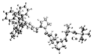
Figure 1: Diagram of the polypeptide donor-spacer-acceptor (DSA) complex referred to as complex 1 in the text.

Testing microscopic solvation theories requires comparison to computer simulations on model, yet realistic, systems. The current experimental database does not provide sufficient accuracy to test various approximations entering theoretical algorithms. On the other hand, computer experiment offers essentially exact (within the accuracy of simulation protocols) integration of the same Hamiltonian as the one used in the analytical theory. Therefore, the present calculations of the ET thermodynamics are compared to recent very extensive Molecular Dynamics (MD) simulations Ungar et al. (1999) of a donor-spacer-acceptor (DSA) complex consisting of transition-metal donor (D) and acceptor (A) sites linked by a polyproline peptide spacer (S) (Fig. 1):

$$\mathrm{(bpy)_{2}Ru^{2+}(bpy^{\prime})-(pro)_{4}-O^{-}Co^{3+}(NH_{3})_{5}},$$

where in the donor bpy=2,2^′-bipyridine and bpy^′=4^′-methyl-2,2^′-bipyridyl. The spacer is a polyproline chain whose first member (the N-terminus) is connected to the bpy^′ carbonyl, and whose fourth member is terminated by a carboxylate moiety bound to the $\mathrm{-Co^{3+}(NH_{3})_{5}}$ acceptor. This system, modeling ET in redox proteins, is a representative member of a homologous series of DSA complexes for which ET rates as a function of temperature have been reported Ogawa et al. (1993). This complex will be referred to as complex 1 in the text.

The analytical NRFT model is shown to agree exceptionally well with MD simulations for complex 1 (Figure 1) in TIP3P water. In order to provide a rigorous comparison between simulations and analytical theory, the set of solute charges employed in the simulations was also used in the analytical calculations. In addition, the polarization structure factors of TIP3P water were obtained from separate MD simulations to be used as input in the analytical theory. Once the accuracy and robustness of the analytical procedures are tested on MD simulations, the next step is to see if the model is capable of reflecting the behavior of real systems. To this end, we have developed a parameterization scheme for polarization structure factors applicable to polarizable polar solvents. Once this is done, the theory can be extended to calculations at varying thermodynamic conditions of the solvent (e.g., temperature) and should generate a set of predictions which can be tested experimentally.

We use the polypeptide DSA to focus on two problematic areas of dielectric continuum models: dependence of the reorganization energy on the solvent polarizability Bader and Berne (1996); Gupta and Matyushov (2004) and the entropy of nuclear solvation Matyushov (1993); Vath et al. (1999). For both areas there is a fundamental, both quantitative and qualitative, disagreement between microscopic models and continuum calculations. Unfortunately, no experimental evidence on the dependence of the solvent reorganization energy on solvent refractive index is available in the literature. There is, on the other hand, a limited number of experimental Grampp and Jaenicke (1984); Liang et al. (1989); Dong and Hupp (1992); Elliott et al. (1998); Nelsen et al. (1999); Derr and Elliott (1999); Vath et al. (1999); Vath and Zimmt (2000); Zhao et al. (2001); Coropceanu et al. (2003); Mertz (2005) and simulation Leontiev and Basilevskii (2005) studies on the entropy of reorganization. Most of the available experimental (laboratory and simulation) evidence points to a positive reorganization entropy (i.e., a negative slope of the reorganization energy vs temperature) in polar solvents, in agreement with the prediction of microscopic theory Matyushov (1993) and in disagreement with negative entropies from continuum calculations Kumar et al. (1998); Vath et al. (1999). We are aware, however, of a few measurements performed on charged donor-acceptor complexes indicating either zero or negative reorganization entropies Dong and Hupp (1992); Coropceanu et al. (2003); Mertz (2005). Our current calculations on complex 1 (Fig. 1) give absolute values of the reorganization entropy much higher than continuum calculations. This great discrepancy calls for additional tests of the theory against experimental data, which will be a subject of future work.

II Golden Rule Rate Constant

The Golden Rule rate constant of ET is Kubo and Toyozawa (1955)

$$k_{\text{ET}}=\frac{2\pi V_{12}^{2}}{\hbar^{2}}\mathrm{FCWD}(0),$$ (1)

where FCWD stands for the density-of-states weighted Franck-Condon (FC) factor

$$\mathrm{FCWD}(\omega)=\int\frac{dt}{2\pi}\left\langle e^{iH_{2}t/\hbar}e^{-iH_{1}t/\hbar}\right\rangle_{n}e^{-i\omega t}.$$ (2)

Here, $\langle\dots\rangle_{n}$ is an ensemble average over the nuclear degrees of freedom of the system (denoted by subscript “n”), which include the manifold of $N$ normal vibrational modes of the donor-acceptor complex $Q=\{\mathbf{q}_{1},\dots\mathbf{q}_{N}\}$ and the nuclear component of the dipolar polarization of the solvent $\mathbf{P}_{n}$. The ensemble average is carried out over the configurations in equilibrium with the initial state. Further, $H_{i}$ ($i=1,2$) are the diagonal matrix elements of the unperturbed system Hamiltonian $H$ taken on the two-state electronic basis $\{\Psi_{1},\Psi_{2}\}$: $H_{i}=\langle\Psi_{i}|H|\Psi_{i}\rangle$ ($i=1$ and $i=2$ stand for the initial and final electronic states, respectively). The sum of $H$ and the perturbation $V$ makes the whole system Hamiltonian, $H^{\prime}=H+V$, and $V_{12}=\langle\Psi_{1}|V|\Psi_{2}\rangle$ is the off-diagonal matrix element in the Golden Rule expression.

The system Hamiltonian of a donor-acceptor complex in a condensed-phase solvent can be separated into the gas-phase component, $H_{g}$, the solute-solvent interaction, $H_{0s}$ (“0” stands for the solute, “s” stands for the solvent), and the bath Hamiltonian, $H_{B}$, describing thermal fluctuations of the solvent:

$$H=H_{g}+H_{0s}+H_{B}.$$ (3)

The gas-phase Hamiltonian is the sum of the kinetic energy of the electrons, kinetic energy of the nuclei, and the full electron-nuclear Coulomb energy. The solute-solvent Hamiltonian for ET in dipolar solvents is commonly given by the coupling of the operator of the solute electric field $\mathbf{\hat{E}}_{0}$ to the dipolar polarization of the solvent $\mathbf{P}$

$$H_{0s}=-\mathbf{\hat{E}}_{0}*\mathbf{P}.$$ (4)

The bath Hamiltonian represents Gaussian statistics of the collective mode $\mathbf{P}$ with the linear response function $\bm{\chi}(\mathbf{r},\mathbf{r}^{\prime})$

$$H_{B}=\frac{1}{2}\mathbf{P}*\bm{\chi}^{-1}*\mathbf{P}.$$ (5)

The asterisk between the bold capital letters denotes tensor contraction (scalar product for vectors) and space integration over the volume $\Omega$ occupied by the solvent

$$\mathbf{E}*\mathbf{P}=\int_{\Omega}\mathbf{E}\cdot\mathbf{P}d\mathbf{r}.$$ (6)

Assuming that the intramolecular vibrations are decoupled from solvent nuclear modes allows one to cast the FCWD as a convolution of the vibrational, $G_{v}(\omega)$, and solvent, $G_{s}(\omega)$, FC densities Bixon and Jortner (1999):

$$\mathrm{FCWD}(\omega)=\int_{-\infty}^{\infty}d\omega^{\prime}G_{v}(\omega^{\prime})G_{s}(\omega-\omega^{\prime}-\Delta G/\hbar),$$ (7)

where the diabatic equilibrium free energy gap is the sum of the gas-phase component $\Delta G_{g}$ and difference in solvation energies $\Delta G_{s}$

$$\Delta G=\Delta G_{g}+\Delta G_{s}.$$ (8)

In the absence of vibrational frequency change, the former component is equal to the 0-0 transition energy in the gas phase.

The FC density for each nuclear mode is given in terms of a broadening function $g_{n}(t)$ Ovchinnikov and Ovchinnikova (1969); Mukamel (1995)

$$G_{n}(\omega^{\prime})=\int_{-\infty}^{\infty}\frac{dt}{2\pi}\exp\left[i(\lambda_{n}/\hbar-\omega^{\prime})t-g_{n}(t)\right],$$ (9)

where

$$\begin{split}g_{n}(t)=&\frac{1}{\pi}\int_{0}^{\infty}\frac{dz}{z^{2}}(1-\cos zt)\chi_{n}^{\prime\prime}(z)\coth\frac{\hbar z}{2k_{\text{B}}T}\\ &+\frac{i}{\pi}\int_{0}^{\infty}\frac{dz}{z^{2}}(zt-\sin zt)\chi_{n}^{\prime\prime}(z).\end{split}$$ (10)

In Eq. (9), $\lambda_{n}$ is the nuclear reorganization energy

$$\lambda_{n}=\frac{\hbar}{\pi}\int_{0}^{\infty}\frac{dz}{z}\chi_{n}^{\prime\prime}(z)$$ (11)

and $\chi_{n}^{\prime\prime}(z)$ is the imaginary part of the frequency-dependent linear response function (spectral density) corresponding to the nuclear mode $n$ (in general, many such modes contribute to the solvent (s) and vibrational (v) FC densities).

For a set of vibrational normal modes with frequencies $\omega_{q}$ and reorganization energies $\lambda_{q}$, the spectral density is Mukamel (1995)

$$\chi_{v}^{\prime\prime}(z)=\pi\sum_{q}S_{q}\omega_{q}^{2}\left[\delta(z-\omega_{q})-\delta(z+\omega_{q})\right],$$ (12)

where $S_{q}=\lambda_{q}/\hbar\omega_{q}$ is the Huang-Rhys factor. When all nuclear modes are classical, $g_{n}(t)=k_{\text{B}}T\lambda_{n}t^{2}/\hbar^{2}$ and one reaches the classical, high temperature limit of the Marcus theory

$$\begin{split}\mathrm{FCWD}_{1}(\omega)=&\left[4\pi(\lambda_{s}+\lambda_{v})k_{\text{B}}T\right]^{-1/2}\\ &\exp\left[-\frac{(\Delta G+\lambda_{s}+\lambda_{v}-\hbar\omega)^{2}}{4k_{\text{B}}T(\lambda_{s}+\lambda_{v})}\right],\end{split}$$ (13)

where $\lambda_{v}=\sum_{q}\lambda_{q}$ is the total vibrational reorganization energy.

When the solvent mode is classical and the vibrations are quantized, one can use the small $t$ expansion in Eq. (9), valid in the limit when $\omega_{q}$ is much smaller than the vertical energy gap [$|\lambda_{v}-\omega^{\prime}|$ in Eq. (9)]. With $\hbar\omega_{q}/k_{\text{B}}T\gg 1$, one gets

$$g_{v}(t)\simeq(t^{2}/2\hbar)\omega_{v}\lambda_{v},$$ (14)

where

$$\omega_{v}=(\lambda_{v})^{-1}\sum_{q}\omega_{q}\lambda_{q}$$ (15)

is the effective vibrational frequency. With the vibrational broadening function in the form of Eq. (14) the FCWD becomes Holstein (1959); Hopfield (1974); Siders and Marcus (1981); Marcus (1989)

$$\begin{split}\mathrm{FCWD}_{1}(\omega)=&\left[\pi(4\lambda_{s}k_{\text{B}}T+2\hbar\omega_{v}\lambda_{v})\right]^{-1/2}\\ &\exp\left[-\frac{(\Delta G+\lambda_{s}+\lambda_{v}-\hbar\omega)^{2}}{4k_{\text{B}}T\lambda_{s}+2\hbar\omega_{v}\lambda_{v}}\right].\end{split}$$ (16)

The above equation, present in some early papers on ET Hopfield (1974); Siders and Marcus (1981), is not very accurate as was pointed out by Jortner Jortner (1976). The set of equations given below, which can be found in work by Lax Lax (1952), Davydov Davydov (1953), and Kubo and Toyozawa Kubo and Toyozawa (1955), provides a better description of the vibronic envelope.

When the normal mode vibrations are represented by a single effective vibration with frequency defined by Eq. (15), the vibrational FCWD is a weighted sum of resonant vibrational transitions

$$G_{v}(\omega)=\sum_{m=-\infty}^{\infty}A_{m}\delta(\omega-m\omega_{v}),$$ (17)

where

$$A_{m}=e^{-S\coth\chi_{v}+m\chi_{v}}I_{m}\left(\dfrac{S}{\sinh\chi_{v}}\right),$$ (18)

$S=\lambda_{v}/\hbar\omega_{v}$, $\chi_{v}=\hbar\omega_{v}/2k_{\text{B}}T$, and $I_{m}(x)$ is the modified Bessel function of order $m$.

The FCWD for the classical nuclear modes of the solvent is given by the expression

$$G_{s}(\omega-\Delta G/\hbar)=\hbar\langle\delta(\Delta E(\mathbf{P}_{n})-\hbar\omega)\rangle,$$ (19)

where

$$\Delta E(\mathbf{P}_{n})=\Delta G+\lambda_{s}-\Delta\mathbf{E}_{0}*\delta\mathbf{P}_{n}$$ (20)

and $\langle\dots\rangle_{1}$ denotes an ensemble average over the fluctuations of the nuclear solvent polarization $\mathbf{P}_{n}$ coupled to the difference in initial and final state electric fields of the donor-acceptor complex, $\Delta\mathbf{E}_{0}=\mathbf{E}_{02}-\mathbf{E}_{01}$. In Eq. (20), $\lambda_{s}$ stands for the solvent reorganization energy (see below), and $\delta\mathbf{P}_{n}$ is the fluctuation of the nuclear polarization with respect to its equilibrium value. With the Gaussian Hamiltonian for polarization fluctuations [Eq. (5)], $G_{s}(\omega-\Delta G/\hbar)$ is a Gaussian function leading to a total FCWD in the form of a weighted sum of Gaussians

$$\begin{split}\mathrm{FCWD}_{i}(\omega)&=\left[4\pi\lambda_{s}k_{\text{B}}T\right]^{-1/2}\sum_{m=-\infty}^{\infty}A_{m}\\ &\exp\left(-\frac{\left(\Delta G+\lambda_{s}+m\hbar\omega_{v}-\hbar\omega\right)^{2}}{4\lambda_{s}k_{\text{B}}T}\right).\end{split}$$ (21)

When the energy of vibrational excitations is much greater than $k_{\text{B}}T$ [$\chi_{v}\gg 1$ in Eq. (18)] the FC envelope turns into a sum of Gaussians with weights given by the Poisson distribution Bixon and Jortner (1999)

$$A_{m}=e^{-S}\frac{S^{m}}{m!},\quad m>0.$$ (22)

III Solvation Thermodynamics

Inserting a solute into a molecular solvent results in solvent perturbation that can roughly be split into two components with drastically different length scales. The first component is due to repulsion of the solvent from the solute core caused by short-range, but strong repulsive forces. This perturbation creates a local density profile in the solvent around the solute which may or may not induce a polarization field acting on the solute charges. The electric field of solute charges creates yet another perturbation. The solute electric field is sufficiently long-ranged to induce the dipolar polarization $\mathbf{P}(\mathbf{r})$ in a quasi-macroscopic region of the solvent around the solute. Gradients of the solute field couple to the higher-order (quadrupolar, etc.) polarization, but this interaction is more short-ranged Perng et al. (1996a, b); Matyushov and Voth (1999); Milischuk and Matyushov (2005a).

The dipolar polarization is caused by alignment of the permanent and induced solvent dipoles along the solute field. This alignment occurs on two quite different time scales: $\simeq 10^{-15}$ s for induced dipoles and $\simeq 10^{-11}-10^{-12}$ s for permanent dipoles. Accordingly, the polarization field splits into a fast relaxing electronic polarization (induced dipoles, $\mathbf{P}_{e}$) and a much slower nuclear polarization (permanent dipoles, $\mathbf{P}_{n}$) com (a). The electronic solvent polarization is always in equilibrium with the changing distribution of the electronic density in the donor-acceptor complex. The energy conservation condition of the Golden Rule formula is thus imposed on the energies with equilibrated electronic polarization. Therefore, before being used in the Golden Rule expression, the Hamiltonian matrix should be averaged over the fast electronic component of the dipolar polarization Gehlen et al. (1992); Matyushov and Ladanyi (1998). For the energy $E_{i}$ depending on the instantaneous configuration of the nuclear subsystem one gets

$$e^{-\beta E_{i}}=\mathrm{Tr}_{\text{el}}\left[e^{-H_{i}/k_{\text{B}}T}\right],$$ (23)

where Tr${}_{\text{el}}$ denotes the statistical average over the electronic degrees of freedom of the solvent. Before going into the details of separate calculations for electronic and nuclear components of the polarization, we outline the general formalism of polarization response to an external electric field.

Figure 2: Two approaches to the calculation of the response function: as polarization response to an external electric field perturbation (a) and as correlation of polarization fluctuations near the solute hard core from which the polarization field is excluded (b).

III.1 Formalism

In the linear response approximation (LRA), the solvent polarization $\mathbf{P}(\mathbf{r})$ is a linear functional of the perturbing electric field $\mathbf{E}_{0}$ (vacuum electric field of the solute for solvation):

$$\mathbf{P}(\mathbf{r})=\bm{\chi}*\mathbf{E}_{0}=\int\bm{\chi}(\mathbf{r},\mathbf{r}^{\prime})\cdot\mathbf{E}_{0}(\mathbf{r}^{\prime})d\mathbf{r}^{\prime}.$$ (24)

Here, $\bm{\chi}(\mathbf{r},\mathbf{r}^{\prime})$ is a two-rank tensor describing the non-local linear response of the solvent to the solute electric field, dot denotes tensor contraction over the common Cartesian projections. This function is different from dielectric susceptibility appearing in Maxwell’s equations in two respects. First, $\bm{\chi}(\mathbf{r},\mathbf{r}^{\prime})$ describes the polarization response to the field of external charges and not to the total electric field $\mathbf{E}=\mathbf{E}_{0}+\mathbf{E}_{P}$ combining the external field with the electric field $\mathbf{E}_{P}$ created by the solvent polarization ($\bm{\chi}$ corresponds to $\bm{\chi}^{0}$ of Madden and Kivelson Madden and Kivelson (1984)). Second, $\bm{\chi}(\mathbf{r},\mathbf{r}^{\prime})$ is affected by the presence of the solute and thus $\bm{\chi}(\mathbf{r}_{1},\mathbf{r}^{\prime})$ is generally not equal to $\bm{\chi}(\mathbf{r}_{2},\mathbf{r}^{\prime\prime})$ even if $\mathbf{r}_{1}-\mathbf{r}^{\prime}=\mathbf{r}_{2}-\mathbf{r}^{\prime\prime}$.

Equation (24) determines the response function in terms of an external electrostatic perturbation and polarization induced by it (Fig. 2a). An alternative view of the response function is through the fluctuation-dissipation theorem which relates the response to the correlation function of polarization fluctuations in the solute vicinity

$$\bm{\chi}(\mathbf{r},\mathbf{r}^{\prime})=(k_{\text{B}}T)^{-1}\langle\delta\mathbf{P}(\mathbf{r})\delta\mathbf{P}(\mathbf{r}^{\prime})\rangle.$$ (25)

An important result of the LRA is that this correlation function does not depend on the long-range electrostatic field of the solute. The ensemble average $\langle\dots\rangle$ in the presence of the real solute with its charge distribution is equivalent to the ensemble average $\langle\dots\rangle_{0}$ in the presence of a fictitious solute which has the geometry of the real solute (and therefore the complete repulsion potential) but no partial charges. This notion provides a convenient route to the calculations of the response function for complex solutes. Instead of calculating the polarization in response to a non-trivial field $\mathbf{E}_{0}(\mathbf{r})$, one can calculate the correlation of polarization fluctuations in the presence of a fictitious solute with only the hard repulsive core of the real solute retained. The correlation function is then calculated with the requirement of zero polarization within the solute (Fig. 2b)

$$\bm{\chi}(\mathbf{r},\mathbf{r}^{\prime})=(k_{\text{B}}T)^{-1}\langle\delta\mathbf{P}(\mathbf{r})\delta\mathbf{P}(\mathbf{r}^{\prime})\rangle_{0}.$$ (26)

This is the essence of the approach adopted in the present formalism, making the response function solely determined by the molecular structure inherent to the pure solvent and the short-range perturbation produced by the repulsive core of the solute.

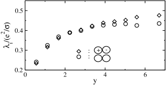
Figure 3: $\lambda_{1}$ for a neutral diatomic D-A (circles) and $\lambda_{2}$ for a polar diatomic D⁺-A^- (diamonds) for a donor-acceptor complex represented by two contact spheres with radii $R_{0}/\sigma=0.9$. Solvent is a fluid of dipolar hard spheres of diameter $\sigma$ and dipole moment $m$. The simulations, reported in Ref. Matyushov, 2004b, were carried out at different $m$ and at constant density $\rho\sigma^{3}=0.8$. The change in solvent polarity is reflected by the dipolar density $y=(4\pi/9)m^{2}\rho/k_{\text{B}}T$.

The applicability of the LRA to solvation of large donor-acceptor complexes common for ET research in molecular solvents is well supported by existing evidence from computer simulations Hwang and Warshel (1987); Kuharski et al. (1988); Marchi et al. (1993); Yelle and Ichiye (1997); Hartnig and Koper (2001). The direct consequence of the LRA are the following relations for the moments of the solute-solvent interaction potential $v_{0s}$:

$$-k_{\text{B}}T\langle v_{0s}\rangle=\langle\left(\delta v_{0s}\right)^{2}\rangle=\langle\left(\delta v_{0s}\right)^{2}\rangle_{0}.$$ (27)

When the solute-solvent interaction is limited to the coupling of the solute charges to the solvent dipolar polarization, $v_{0s}=\langle\Psi|H_{0s}|\Psi\rangle$ in Eq. (4).

The independence of the response function with respect to the solute charge is propagated into equality of the variance of $v_{0s}$ in equilibrium with fully charged solute, $\langle\dots\rangle$, and in equilibrium with uncharged solute, $\langle\dots\rangle_{0}$. Figure 3 shows the results of simulations from Ref. Matyushov, 2004b for a model diatomic donor-acceptor complex D–A in a dense solvent of hard sphere point dipoles. The system is designed to mimic the charge separation, D–A $\to$ D⁺–A^-, and charge recombination, D⁺–A^- $\to$ D–A, reactions. The reorganization energies for charge separation, $\lambda_{1}=\langle\left(\delta v_{0s}\right)^{2}\rangle_{0}/2k_{\text{B}}T$, and for charge recombination, $\lambda_{2}=\langle\left(\delta v_{0s}\right)^{2}\rangle/2k_{\text{B}}T$, turn out to be very similar over a broad range of solvent polarities monitored by the dipolar density parameter $y=(4\pi/9)m^{2}\rho/k_{\text{B}}T$; $\rho$ is the solvent number density, $m$ is the solvent molecule permanent dipole moment.

The inhomogeneous character of the response functions is retained after transformation to $\mathbf{k}$-space. The function $\bm{\chi}(\mathbf{k},\mathbf{k}^{\prime})$ then depends on two wavevectors in contrast to the dependence on a single wave-vector for the homogeneous dielectric response. The calculation of $\bm{\chi}(\mathbf{k},\mathbf{k}^{\prime})$ is still a major challenge for microscopic theories of polar solvation. Despite some very active research in this area for the last 80 years since the formulation of the Born model for solvation of spherical ions Born (1920), no microscopic solution applicable to solutes of arbitrary shape has been presented so far. A promising strategy, adopted already in the Born Born (1920) and Onsager Onsager (1936) models, is to calculate the response functions in terms of properties of the pure solvent. This connection can be achieved by considering the polarization correlation function in the presence of the repulsive core of the solute [Eq. (26)].

The exclusion of the polarization field from the solute volume is provided by the Li-Kardar-Chandler approach Li and Kardar (1992); Chandler (1993), in which the trajectories defining the response function in its path integral representation are restricted from entering the solute. The result of this procedure is an integral equation relating $\bm{\chi}(\mathbf{k},\mathbf{k}^{\prime})$ to the non-local susceptibility of the pure solvent $\bm{\chi}_{s}(\mathbf{k})$ (with a single $\mathbf{k}$-vector for the homogeneous response) and the shape of the solute. The equation for the response function is then equivalent to the Ornstein-Zernike equation for the solute-solvent correlation function with the Percus-Yevick closure for the solute-solvent direct correlation function Chandler (1993).

No general solution for $\bm{\chi}(\mathbf{k},\mathbf{k}^{\prime})$ in the Li-Kardar-Chandler integral equation has been obtained so far. One can, however, employ analytical properties of the response functions to obtain the solvation chemical potential Matyushov (2004a)

$$-\mu_{0s}=\frac{1}{2}\int\frac{d\mathbf{k}d\mathbf{k}^{\prime}}{(2\pi)^{6}}\mathbf{\tilde{E}}_{0}(\mathbf{k})\cdot\bm{\chi}(\mathbf{k},\mathbf{k}^{\prime})\cdot\mathbf{\tilde{E}}_{0}(-\mathbf{k}^{\prime}).$$ (28)

The closed-form result for $\mu_{0s}$ exists when the Fourier transform of the electric field $\mathbf{\tilde{E}}_{0}(\mathbf{k})$ is known in analytical functional form. This is not the case for many real problems, when the distribution of molecular charge is given from force fields or quantum calculations and the Fourier transform of the field is calculated numerically. Unfortunately, the analytical solution is given by the difference of two large numbers almost canceling each other. It therefore becomes not very practical in strongly polar solvents because of accumulation of numerical errors. To facilitate numerical applications, a mean-field solution for $\bm{\chi}(\mathbf{k},\mathbf{k}^{\prime})$ was offered in Ref. Matyushov, 2004b. This solution eliminates the inhomogeneous character of the response function by a non-local renormalization of its transverse component:

$$\bm{\chi}(\mathbf{k},\mathbf{k}^{\prime})=(2\pi)^{3}\delta(\mathbf{k}-\mathbf{k}^{\prime})\left[\chi^{L}(\mathbf{k})\mathbf{J}^{L}+\chi^{T}(\mathbf{k})\mathbf{J}^{T}\right],$$ (29)

where $\mathbf{J}^{L}=\mathbf{\hat{k}}\mathbf{\hat{k}}$ and $\mathbf{J}^{T}=\mathbf{1}-\mathbf{\hat{k}}\mathbf{\hat{k}}$ are, respectively, the longitudinal and transverse projections of a 2-rank tensor with the axial symmetry established by the direction of the wavevector, $\mathbf{\hat{k}}=\mathbf{k}/k$. The 6D integral of Eq. (28) is then reduced to the computationally tractable 3D integral.

The transverse, $\chi^{T}(\mathbf{k})$, and longitudinal, $\chi^{L}(\mathbf{k})$, projections in Eq. (29) are related to corresponding components of the susceptibility of the pure polar solvent

$$\chi^{T}(\mathbf{k})=\chi_{s}^{T}(k)\frac{\chi_{s}^{L}(0)}{\chi_{\text{tr}}}-f_{s}\chi_{s}^{L}(k)\frac{\mathbf{F}_{0}\cdot\mathbf{J}^{L}\cdot\mathbf{\tilde{E}}_{0}(\mathbf{k})}{\mathbf{F}_{0}\cdot\mathbf{J}^{T}\cdot\mathbf{\tilde{E}}_{0}(\mathbf{k})}$$ (30)

and

$$\chi^{L}(\mathbf{k})=\chi_{s}^{L}(k).$$ (31)

In Eq. (30), $\chi_{\text{tr}}=(1/3)\mathrm{Tr}[\bm{\chi}_{s}(0)]$ and

$$f_{s}=\frac{2[\chi_{s}^{T}(0)-\chi_{s}^{L}(0)]}{3\chi_{\text{tr}}}.$$ (32)

Further, $\mathbf{\tilde{E}}_{0}(\mathbf{k})$ denotes the Fourier transform of the electric field of the solute calculated on the volume of the solvent $\Omega$ obtained by excluding the hard repulsive core of the solute from the solvent

$$\mathbf{\tilde{E}}_{0}(\mathbf{k})=\int_{\Omega}\mathbf{E}_{0}(\mathbf{r})e^{i\mathbf{k}\cdot\mathbf{r}}d\mathbf{r}.$$ (33)

The mean-field approximation adopted in deriving Eqs. (29)–(33) consists of replacing a generally non-uniform field of the solvent within the solute by its spatial average $\mathbf{F}_{0}$ [Eq. (30)]. The neglect of the gradients of the field induced by the solvent within the solute amounts to taking the dipolar projection of the solute field according to the following relation:

$$\mathbf{F}_{0}=\ \int_{\Omega}\mathbf{E}_{0}(\mathbf{r})\cdot\mathbf{D}_{\mathbf{r}}\frac{d\mathbf{r}}{r^{3}},$$ (34)

where

$$\mathbf{D}_{\mathbf{r}}=3\mathbf{\hat{r}}\mathbf{\hat{r}}-\mathbf{1}.$$ (35)

is the dipolar tensor. The electric field $\mathbf{F}_{0}$ is a generalization of the Onsager reaction field for the case of non-spherical solutes with non-dipolar charge distribution. $\mathbf{F}_{0}$ reduces to the Onsager field for spherical dipolar solutes.

The mean-field renormalization of the transverse component of the response function in Eq. (30) resolves the fundamental difficulty of microscopic solvation theories arising from the fact that the short-range repulsive perturbation caused by the solute produces a major change in the polarization response functions compared to those of the pure solvent. For instance, a direct replacement of $\bm{\chi}(\mathbf{k})$ with $\bm{\chi}_{s}(\mathbf{k})$ in the homogeneous approximation (see Ref. Raineri et al., 1994 for discussion) results in divergent behavior of $\lambda_{s}$ with increasing solvent dipole moment Matyushov (1996). The divergence arises from the transverse component of the response (“transverse catastrophe”) which has to be included once the dielectric cavity does not coincide with an equipotential surface of the solute charge distribution Kharkats et al. (1976). In continuum calculations, the divergent behavior is eliminated by imposing boundary conditions at the dielectric cavity on the solution of the Poisson equation.

Although the problem with the transverse response has long been recognized in the literature Kharkats et al. (1976); Matyushov (1996); Kuznetsov and Medvedev (1996), many microscopic formulations of solvation thermodynamics and dynamics have avoided the problem by neglecting the transverse response Chandra and Bagchi (1989); Bagchi and Chandra (1989); Fried and Mukamel (1990) which is also neglected in some continuum calculations, e.g. the Generalized Born approximation Schaefer and Karplus (1996). Equations (29)–(33) provide a general solution of the problem which agrees well with available simulations of polar solvation Matyushov (2004a, b) and experiment on solvation dynamics Matyushov (2005). The formalism is based on the homogeneous solvent susceptibility as input and, once the susceptibility is defined from computer experiment or liquid-state theories, can be applied to solvation in an arbitrary isotropic dielectric.

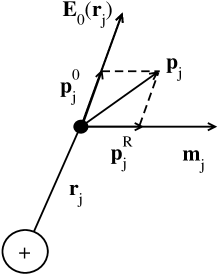
Figure 4: Components of the induced dipole moment at solvent molecule $j$. $\mathbf{p}_{j}^{0}$ is produced by the external electric field $\mathbf{E}_{0}(\mathbf{r}_{j})$; $\mathbf{p}_{j}^{R}$ is produced by the reaction field induced in the solvent by the permanent dipole $\mathbf{m}_{j}$.

III.2 Polarization structure factors

The dipole moment at a given molecule $j$ in a polar-polarizable solvent is a sum of the permanent dipole $\mathbf{m}_{j}$ and the induced dipole $\mathbf{p}_{j}$

$$\bm{\mu}_{j}=\mathbf{m}_{j}+\mathbf{p}_{j}.$$ (36)

The total induced dipole then splits into $\mathbf{p}_{j}^{0}$ created by the external electric field $\mathbf{E}_{0}(\mathbf{r}_{j})$ and $\mathbf{p}_{j}^{R}$ induced by the reaction field (superscript “R”) caused by the dipole $\mathbf{m}_{j}$ itself (Fig. 4):

$$\mathbf{p}_{j}=\mathbf{p}_{j}^{0}+\mathbf{p}_{j}^{R}$$ (37)

The reaction field caused by the dipole $\mathbf{m}_{j}$ relaxes on the time-scale of translational-rotational motion of molecule $j$. Therefore, the induced dipole $\mathbf{p}_{j}^{R}$, which follows adiabatically the reaction field, should be attributed com (b) to the slow nuclear polarization of the solvent $\mathbf{P}_{n}$. In contrast, the component $\mathbf{p}_{j}^{0}$, following adiabatically the external field, is attributed to the the fast solvent polarization $\mathbf{P}_{e}$. The sum of the permanent dipole $\mathbf{m}_{j}$ and the induced dipole $\mathbf{p}_{j}^{R}$ makes the effective condensed-phase dipole Stell et al. (1981)

$$\mathbf{m}_{j}^{\prime}=\mathbf{m}_{j}+\mathbf{p}_{j}^{R}=m^{\prime}\mathbf{\hat{e}}_{j},$$ (38)

where $\mathbf{\hat{e}}_{j}$ is the unit vector along the direction of $\mathbf{m}_{j}$. The dipole moment $m^{\prime}$ in principle depends on the instantaneous configuration of the liquid. However, we will not consider fluctuations of $m^{\prime}$ here and, following self-consistent models of polarizable liquids Stell et al. (1981), will replace $m^{\prime}$ with its statistical average value.

The attribution of the electronic polarization in equilibrium with the electric field of the permanent dipoles to the nuclear (slow) polarization of the solvent is an essential part of the Pekar partitioning of the solvent polarization into fast and slow components Pekar (1946, 1963). Other partitioning schemes have been proposed Brady and Carr (1985), but they all lead to the same value of the solvation energy when correctly implemented Aguilar (2001). Computer simulation protocols in which the induced polarization is self-consistently adjusted to the instantaneous nuclear configuration provide direct access to the slow polarization in Pekar’s definition Milischuk and Matyushov (2005b). Self-consistent simulations of polarizable solvents are used here to test the analytical procedure employed for the response functions of the nuclear polarization (Sec. IV.1).

The total dipolar response function of the homogeneous solvent is a 2-rank tensor describing correlations of dipole moments $\bm{\mu}_{j}$:

$$\bm{\chi}_{s}(\mathbf{k})=(\beta/\Omega)\left\langle\sum_{j,k}\bm{\mu}_{j}\bm{\mu}_{k}e^{i\mathbf{k}\cdot\mathbf{r}_{jk}}\right\rangle,$$ (39)

where $\mathbf{r}_{jk}=\mathbf{r}_{j}-\mathbf{r}_{k}$ and brackets refer to an ensemble average. Because of the isotropic symmetry of the solvent, $\bm{\chi}_{s}(\mathbf{k})$ splits into longitudinal and transverse components Madden and Kivelson (1984)

$$\bm{\chi}_{s}(\mathbf{k})=\chi_{s}^{L}(k)\mathbf{J}^{L}+\chi_{s}^{T}(k)\mathbf{J}^{T}.$$ (40)

It is convenient to factor the response function into the effective density of dipoles $y_{\text{eff}}$, which is mostly affected by the magnitude of the solvent dipole, and the structure factor, which reflects dipolar correlations and can be expressed through angular projections of the pair distribution function Matyushov (2004b)

$$\bm{\chi}_{s}(\mathbf{k})=\frac{3y_{\text{eff}}}{4\pi}\left[S^{L}(k)\mathbf{J}^{L}+S^{T}(k)\mathbf{J}^{T}\right].$$ (41)

The structure factors $S^{L,T}(k)$ (Fig. 5) are defined based on the unit vectors $\mathbf{\hat{u}}_{j}=\bm{\mu}_{j}/\mu_{j}$ in the direction of the respective total dipole moments

$$\begin{split}S^{L}(k)=&\frac{3}{N}\left\langle\sum_{i,j}(\mathbf{\hat{u}}_{i}\cdot\mathbf{\hat{k}})(\mathbf{\hat{k}}\cdot\mathbf{\hat{u}}_{j})e^{i\mathbf{k}\cdot\mathbf{r}_{ij}}\right\rangle,\\ S^{T}(k)=&\frac{3}{2N}\left\langle\sum_{i,j}\left[(\mathbf{\hat{u}}_{i}\cdot\mathbf{\hat{u}}_{j})-(\mathbf{\hat{u}}_{i}\cdot\mathbf{\hat{k}})(\mathbf{\hat{k}}\cdot\mathbf{\hat{u}}_{j})\right]e^{i\mathbf{k}\cdot\mathbf{r}_{ij}}\right\rangle.\end{split}$$ (42)

The effective dipole density in Eq. (41) is

$$y_{\text{eff}}=y_{p}+(4\pi/3)\rho\alpha,\quad y_{p}=(4\pi/9)\rho(m^{\prime})^{2}/k_{\text{B}}T,$$ (43)

where $\alpha$ is the dipolar polarizability. Only the permanent dipole moment is renormalized by the mean field of the solvent in the above equation, which corresponds to Wertheim’s 1-RPT theory Wertheim (1979) (2-RPT theory renormalizes the polarizability $\alpha$ to $\alpha^{\prime}$, but the 1-RPT version of the theory is in better agreement with simulations Gupta and Matyushov (2004)).

The nuclear response function reflects correlated orientations and positions of dipoles $\mathbf{m}_{j}^{\prime}$:

$$\bm{\chi}_{n}(\mathbf{k})=(\beta/\Omega)\left\langle\sum_{j,k}\mathbf{m}_{j}^{\prime}\mathbf{m}_{k}^{\prime}e^{i\mathbf{k}\cdot\mathbf{r}_{jk}}\right\rangle.$$ (44)

Similarly to Eq. (41), $\bm{\chi}_{n}(\mathbf{k})$ can be separated into the longitudinal and transverse components

$$\bm{\chi}_{n}(\mathbf{k})=\frac{3y_{p}}{4\pi}\left[S_{n}^{L}(k)\mathbf{J}^{L}+S_{n}^{T}(k)\mathbf{J}^{T}\right].$$ (45)

The nuclear structure factors are defined by Eq. (42), in which the unit vectors $\mathbf{\hat{u}}_{j}$ are replaced by the unit vectors $\mathbf{\hat{e}}_{j}$ [Eq. (38)].

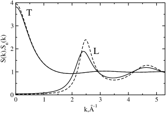
Figure 5: Longitudinal (L) and transverse (T) polarization structure factors calculated by using the PPSF with the parameters of ambient water. The solid lines refer to the total structure factors $S^{L,T}(k)$, the dashed lines refer to the nuclear structure factors $S_{n}^{L,T}(k)$.

The $k=0$ values of the structure factors are related to the macroscopic dielectric properties of the solvent. The total polarization response is defined through the static dielectric constant $\epsilon_{s}$

$$\begin{split}S^{L}(0)&=\frac{\epsilon_{s}-1}{3\epsilon_{s}y_{\text{eff}}},\\ S^{T}(0)&=\frac{\epsilon_{s}-1}{3y_{\text{eff}}}.\end{split}$$ (46)

The nuclear structure factors depend, in addition, on the high-frequency dielectric constant $\epsilon_{\infty}$ Milischuk and Matyushov (2005b)

$$\begin{split}S_{n}^{L}(0)&=\frac{c_{0}}{3y_{p}},\\ S_{n}^{T}(0)&=\frac{\epsilon_{s}-\epsilon_{\infty}}{3y_{p}},\end{split}$$ (47)

where

$$c_{0}=1/\epsilon_{\infty}-1/\epsilon_{s}$$ (48)

is the Pekar factor.

Both $S_{n}^{L,T}(k)$ and $S^{L,T}(k)$ tend to unity at $k\to\infty$. This limit is the result of the point multipole approximation for the intramolecular charge distribution within the solvent molecules. In contrast, charge-charge structure factors defined on interaction-site models of liquids decay to zero at $k\to\infty$ (Refs. Perng et al., 1996a; Raineri and Friedman, 1999; Perng and Ladanyi, 1999). The region of $k$-values where this distinction becomes important is, however, insignificant for the calculation of solvation thermodynamics (see below). The nuclear and the total structure factors differ in the range of small $k$-values and around the longitudinal peak as a result of the influence of the high-frequency dielectric constant of the solvent (Fig. 5). The effect of $\epsilon_{\infty}$ on the longitudinal peak is insignificant for the calculation of the reorganization energy. Therefore, it is the range of small $k$-values and, in addition, the dependence of the liquid-state dipole moment $m^{\prime}$ on the solvent polarizability, that ultimately determine the variation of the solvent reorganization energy with the solvent high-frequency dielectric constant $\epsilon_{\infty}$ (see below).

III.3 ET thermodynamics

The solvation thermodynamics of ET is determined by the solvent reorganization energy and the solvent component of the free energy gap. They are defined in terms of the nuclear and total response functions by the following relations

$$\lambda_{s}=\frac{1}{2}\int\frac{d\mathbf{k}d\mathbf{k}^{\prime}}{(2\pi)^{6}}\Delta\mathbf{\tilde{E}}_{0}(\mathbf{k})\cdot\bm{\chi}_{n}(\mathbf{k},\mathbf{k}^{\prime})\cdot\Delta\mathbf{\tilde{E}}_{0}(-\mathbf{k}^{\prime})$$ (49)

and

$$\Delta G_{s}=-\int\frac{d\mathbf{k}d\mathbf{k}^{\prime}}{(2\pi)^{6}}\Delta\mathbf{\tilde{E}}_{0}(\mathbf{k})\cdot\bm{\chi}(\mathbf{k},\mathbf{k}^{\prime})\cdot\mathbf{\bar{E}}_{0}(-\mathbf{k}^{\prime}).$$ (50)

In Eqs. (49) and (50), $\Delta\mathbf{\tilde{E}}_{0}(\mathbf{k})=\mathbf{\tilde{E}}_{02}(\mathbf{k})-\mathbf{\tilde{E}}_{01}(\mathbf{k})$ and $\mathbf{\bar{E}}_{0}(\mathbf{k})=(\mathbf{\tilde{E}}_{02}(\mathbf{k})+\mathbf{\tilde{E}}_{01}(\mathbf{k}))/2$; $\mathbf{\tilde{E}}_{0i}(\mathbf{k})$ are the Fourier transforms of the solute electric field in the initial ($i=1$) and final ($i=2$) ET states taken over the volume $\Omega$ occupied by the solvent [Eq. (33)].

The mean-field solution for the response functions [Eq. (29)] splits both the solvent reorganization energy and the free energy gap into their corresponding longitudinal and transverse components:

$$\lambda_{s}=\lambda_{s}^{L}+\lambda_{s}^{T}$$ (51)

and

$$\Delta G_{s}=\Delta G_{s}^{L}+\Delta G_{s}^{T}.$$ (52)

Each projection is obtained as a $\mathbf{k}$-integral with the corresponding polarization structure factor. For the “T” projections one gets

$$\lambda_{s}^{T}=\frac{3y_{p}}{8\pi}\,\frac{S_{n}^{L}(0)}{g_{Kn}}\int\frac{d\mathbf{k}}{(2\pi)^{3}}\left|\Delta\tilde{E}_{0}^{T}(\mathbf{k})\right|^{2}S_{n}^{T}(k)$$ (53)

and

$$\begin{split}\Delta G_{s}^{T}&=-\frac{3y_{\text{eff}}}{8\pi}\,\frac{S^{L}(0)}{g_{K}}\int\frac{d\mathbf{k}}{(2\pi)^{3}}\\ &\left[|\tilde{E}_{02}^{T}(\mathbf{k})|^{2}-|\tilde{E}_{01}^{T}(\mathbf{k})|^{2}\right]S^{T}(k).\end{split}$$ (54)

In Eqs. (53) and (54),

$$g_{Kn}=(1/3)\left[S_{n}^{L}(0)+2S_{n}^{T}(0)\right]$$ (55)

and

$$g_{Kn}=(1/3)\left[S^{L}(0)+2S^{T}(0)\right]$$ (56)

are the nuclear and total Kirkwood factors, respectively.

The longitudinal components of free energies, $\lambda_{s}^{L}$ and $\Delta G_{s}^{L}$, include both the longitudinal and transverse projections of the solute field:

$$\lambda_{s}^{L}=\frac{3y_{p}}{8\pi}\int\frac{d\mathbf{k}}{(2\pi)^{3}}\mathcal{E}^{\text{eff}}_{\Delta}(\mathbf{k})S_{n}^{L}(k)$$ (57)

and

$$\Delta G_{s}^{L}=-\frac{3y_{\text{eff}}}{8\pi}\int\frac{d\mathbf{k}}{(2\pi)^{3}}\left(\mathcal{E}_{2}^{\text{eff}}(\mathbf{k})-\mathcal{E}_{1}^{\text{eff}}(\mathbf{k})\right)S^{L}(k).$$ (58)

In Eqs. (57) and (58),

$$\mathcal{E}^{\text{eff}}_{\Delta}(\mathbf{k})=|\Delta\tilde{E}_{0}^{L}(\mathbf{k})|^{2}-f_{n}|\Delta\tilde{E}_{0}^{T}(\mathbf{k})|^{2}\frac{\Delta\mathbf{F}_{0}\cdot\mathbf{J}^{L}\cdot\Delta\mathbf{\tilde{E}_{0}}(\mathbf{k})}{\Delta\mathbf{F}_{0}\cdot\mathbf{J}^{T}\cdot\Delta\mathbf{\tilde{E}}_{0}(\mathbf{k})}$$ (59)

and

$$\mathcal{E}^{\text{eff}}_{i}(\mathbf{k})=|\tilde{E}_{0i}^{L}(\mathbf{k})|^{2}-f_{s}|\tilde{E}_{0i}^{T}(\mathbf{k})|^{2}\frac{\mathbf{F}_{0i}\cdot\mathbf{J}^{L}\cdot\mathbf{\tilde{E}}_{0i}(\mathbf{k})}{\mathbf{F}_{0i}\cdot\mathbf{J}^{T}\cdot\mathbf{\tilde{E}}_{0i}(\mathbf{k})}.$$ (60)

The longitudinal and transverse components of the electrostatic energy density in Eqs. (53)–(58) are defined as

$$\begin{split}|\Delta E_{0}^{L,T}(\mathbf{k})|^{2}&=\Delta\mathbf{\tilde{E}}_{0}(\mathbf{k})\cdot\mathbf{J}^{L,T}\cdot\Delta\mathbf{\tilde{E}}_{0}(-\mathbf{k}),\\ |E_{0i}^{L,T}(\mathbf{k})|^{2}&=\mathbf{\tilde{E}}_{0i}(\mathbf{k})\cdot\mathbf{J}^{L,T}\cdot\mathbf{\tilde{E}}_{0i}(-\mathbf{k}).\end{split}$$ (61)

The effective fields $\mathcal{E}^{\text{eff}}_{\Delta}(\mathbf{k})$ and $\mathcal{E}^{\text{eff}}_{i}(\mathbf{k})$ depend on the symmetry of the charge distribution within the solute analogously to the result of imposing the boundary conditions on the solution of the Poisson equation in continuum electrostatics.

The electric field $\mathbf{F}_{0i}$ in Eq. (60) is a generalization of the Onsager reaction cavity field Onsager (1936) to the case of solutes of non-spherical shape and non-point-dipole charge distribution. This field is obtained by summing up a continuous distribution of dipolar electric fields induced by the solute in the solvent volume:

$$\mathbf{F}_{0i}=\ \int_{\Omega}\mathbf{E}_{0i}(\mathbf{r})\cdot\mathbf{D}_{\mathbf{r}}\frac{d\mathbf{r}}{r^{3}},$$ (62)

where $\mathbf{D}_{\mathbf{r}}$ is given by Eq. (35). Also, $\Delta\mathbf{F}_{0}$ in Eq. (59) is $\Delta\mathbf{F}_{0}=\mathbf{F}_{02}-\mathbf{F}_{01}$. $\mathbf{F}_{0i}$ becomes the standard Onsager reaction field for a point dipole at the center of a spherical cavity. Finally, in Eqs. (59) and (60),

$$f_{s}=\frac{2(\epsilon_{s}-1)}{2\epsilon_{s}+1}$$ (63)

is the usual Onsager polarity parameter Onsager (1936) and the corresponding polarity parameter for the nuclear polarization is

$$f_{n}=\frac{2(\epsilon_{\infty}\epsilon_{s}-1)}{2\epsilon_{\infty}\epsilon_{s}+1}.$$ (64)

IV Calculation procedure

The formalism outlined above is realized in a computational algorithm sketched in Figure 6. It includes two branches, one is for the solvent part of the calculation and another is for the solute part. The two parts are combined together in the integration over the inverted space, which yields the reorganization energy ($\lambda_{s}$) and the total free energy of nuclear plus electronic solvation ($\Delta G_{s}$). We start with describing the solvent branch followed by the outline of the solute part.

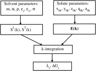
Figure 6: Diagram of the calculation algorithm. Solvent parameters include: $m$ (gas-phase dipole moment), $\alpha$ (gas-phase dipolar polarizability), $\epsilon_{\infty}$ (high-frequency dielectric constant), $\epsilon_{s}$ (static dielectric constant), and $\sigma$ (effective hard sphere diameter of the solvent molecules). Parameters $x_{0k}$, $y_{0k}$, $z_{0k}$ stand for Cartesian coordinated of the solute atoms, $q_{0k}$ are partial charges, and $a_{0k}$ are atomic vdW radii.

IV.1 Solvent

The calculation of the structure factors in the solvent branch in Fig. 6 requires a set of experimental input parameters: $m$ (gas-phase dipole moment), $\alpha$ (gas-phase dipolar polarizability), $\epsilon_{\infty}$ (high-frequency dielectric constant), $\epsilon_{s}$ (static dielectric constant), and $\sigma$ (effective hard sphere diameter of the solvent molecules). The hard sphere diameter is obtained from the experimental compressibility of the solvent by fitting it to the compressibility found from the generalized van der Waals (vdW) equation of state Schmid and Matyushov (1995). Based on these parameters, an analytical procedure has been recently proposed to calculate $S^{L,T}(k)$ Matyushov (2004b). This parameterization, called parametrized polarization structure factors (PPSF), makes use of the analytical solution of the mean-spherical approximation (MSA) for dipolar fluids Wertheim (1971). The MSA solution gives $S^{L,T}(k)$ in terms of the Baxter function $Q(k\sigma,\eta)$ appearing as solution of Percus-Yevick integral equations for hard sphere fluids Gray and Gubbins (1984)

$$S(k\sigma,\eta)=|Q(k\sigma,\eta)|^{-2},$$ (65)

where

$$\begin{split}Q(k\sigma,\eta)=&1-12\eta\int_{0}^{1}e^{ik\sigma t}\\ &\left[a(\eta)(t^{2}-1)/2-b(\eta)(t-1)\right]dt\end{split}$$ (66)

and $a(\eta)=(1+2\eta)/(1-\eta)^{2}$, $b(\eta)=-3\eta/2(1-\eta)^{2}$. For a fluid of hard sphere molecules, $\eta=(\pi/6)\rho\sigma^{3}$ is the packing density, equal to the ratio of the volume of the solvent molecules to the volume of the liquid. In the MSA, the $S^{L,T}(k)$ are obtained by setting $\eta=2\xi$ for $S^{L}(k)$ and $\eta=-\xi$ for $S^{T}(k)$ in Eq. (65). Here, $\xi$ is the MSA polarity parameter which can be related either to the dipolar density $y_{\text{eff}}$ or to the static dielectric constant $\epsilon_{s}$ Wertheim (1971).

Two problems arise when dealing with the reorganization energy calculations using the polarization structure factors from the MSA. First, one needs a general procedure which would provide the nuclear structure factors $S_{n}^{L,T}(k)$ in polarizable solvents in contrast to total structure factors $S^{L,T}(k)$ given by the MSA solution. Such a formalism should thus exclude (quantum) fluctuations of the induced solvent dipoles $\mathbf{p}_{j}^{0}$ which are not included in the nuclear polarization field (Fig. 4). Second, the MSA does not give a consistent description of the dielectric properties of polar solvents, i.e. the polarity parameters $\xi$ calculated from $y_{\text{eff}}$ and $\epsilon_{s}$ are quite different. The PPSF procedure goes around the second problem by considering $y_{\text{eff}}$ and $\epsilon_{s}$ as two independent input parameters used to calculate $S^{L,T}(k)$. A convenient way to introduce the two-parameter scheme is to specify two separate polarity parameters which are obtained from the longitudinal and transverse structure factors at $k=0$:

$$\begin{split}\frac{(1-2\xi^{L})^{4}}{(1+4\xi^{L})^{2}}=&S^{L}(0),\\ \frac{(1+\xi^{T})^{4}}{(1-2\xi^{T})^{2}}=&S^{T}(0).\end{split}$$ (67)

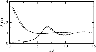
Figure 7: Nuclear longitudinal (L) and transverse (T) structure factors from the PPSF (dashed lines) and MC simulations (solid lines). MC simulations are carried out for a fluid of 1372 hard spheres with permanent dipole $m$, diameter $\sigma$, polarizability $\alpha$, and density $\rho$: $(m^{*})^{2}=\beta m^{2}/\sigma^{3}=1.0$, $\alpha^{*}=\alpha/\sigma^{3}=0.06$, $\rho\sigma^{3}=0.8$. The dielectric properties from the simulations are: $\epsilon_{s}=21.4$, $y_{\text{eff}}=1.57$, and $y_{p}=1.54$; $\epsilon_{\infty}=1.75$ is obtained from the Clausius-Mossotti equation.

Separate definitions of $\xi^{L}$ and $\xi^{T}$ in terms of $S^{L}(0)$ and $S^{T}(0)$ [Eq. (46)] allows us to incorporate contributions to macroscopic dielectric properties which are not present in the model of dipolar HS fluids. Specifically, the magnitude of parameter $y_{\text{eff}}$, calculated according to Wertheim’s 1-RPT algorithm Wertheim (1979), defines the solvent dipolar strength which strongly affects the dielectric constant. However, $\epsilon_{s}$ also depends on such factors as solvent quadrupolar moment Stell et al. (1981), solvent non-sphericity, etc. The influence of these factors is incorporated into $S^{L,T}(0)$ through the dielectric constant. Similarly, the polarity parameters $\xi_{n}^{L}$ and $\xi_{n}^{T}$ are calculated from Eq. (67) with $S^{L,T}(0)$ replaced by $S_{n}^{L,T}(0)$ taken from Eq. (47).

Dipolar projections of the structure factors of molecular liquids modeled by site-site interaction potentials have been studied previously Fonseca and Ladanyi (1990); Raineri and Friedman (1993); Skaf and Ladanyi (1995); Perng and Ladanyi (1999). The PPSF procedure has also been tested against MC simulations of dipolar hard sphere fluids Matyushov (2004b). However, the structure factors arising from the nuclear polarization as well as the applicability of the PPSF to non-spherical molecules with site-site potentials have not been previously tested. This is the aim of the Monte Carlo (MC) and MD simulations carried out in this study. The details of the simulation protocol are given in Appendix A and here we focus only on the results.

Figure 7 shows the comparison of the transverse and longitudinal components of the nuclear structure factors calculated from the PPSF and from MC simulations. The MC simulations (dashed lines in Fig. 7) have been performed on a fluid of 1372 polarizable dipolar hard spheres characterized by dipole moment $m$, diameter $\sigma$, and isotropic polarizability $\alpha$ ($(m^{*})^{2}=\beta m^{2}/\sigma^{3}=1.0$, $\alpha^{*}=\alpha/\sigma^{3}=0.06$, Appendix A). Since the simulation protocol generates the induced polarization in equilibrium with the nuclear configuration of the solvent Gupta and Matyushov (2004), the generated ensamble yields the nuclear polarization in the Pekar partitioning Pekar (1963).

The PPSF nuclear structure factors are calculated by the relations:

$$S_{n}^{T}(k)=|Q(k\sigma,-\xi_{n}^{T})|^{-2}$$ (68)

and

$$S_{n}^{L}(k)=|Q(\kappa k\sigma,2\xi_{n}^{L})|^{-2}.$$ (69)

In Eq. (69), $\kappa=0.95$ is an empirical parameter introduced for a better agreement between the PPSF and MC simulations of non-polarizable dipolar fluids Milischuk and Matyushov (2005b). The simulations and the PPSF agree well in the entire range of solvent polarizabilities $\alpha^{*}=\alpha/\sigma^{3}=0.01-0.08$ studied by simulations Milischuk and Matyushov (2005b).

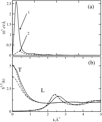
Figure 8: Upper panel: longitudinal (1), $k^{2}\langle\mathcal{E}_{\Delta}^{\text{eff}}(\mathbf{k}))\rangle_{\mathbf{\hat{k}}}$, and transverse (2), $k^{2}\langle(\Delta E^{T}_{0}(k))^{2}\rangle_{\mathbf{\hat{k}}}$ components of the electrostatic energy density of complex 1 entering the $k$-integral in Eqs. (57) and (53), respectively. $\langle\dots\rangle_{\mathbf{\hat{k}}}$ denotes the average over the orientations of the wavevector $\mathbf{k}$. Lower panel: longitudinal (L) and transverse (T) structure factors for TIP3P water at 298 K. The solid lines refer to the results of MD simulations. Dashed lines indicate the results of PPSF calculations with the input parameters corresponding to the TIP3P force field (Table 5, $m=2.35$ D, $\epsilon_{s}=95.4$, $\epsilon_{\infty}=1.0$) and $\sigma=2.87$ Å. The dash-dotted lines refer to the nuclear structure factors of ambient water. The graphs in the upper and lower panels are plotted against the same scale of $k$-values to indicate that the details of the structure factors beyond approximately $k\sigma\simeq\pi$ are insignificant for the calculation of the reorganization energy.

The MSA solution in Eq. (65) was derived for a model liquid of dipolar hard spheres. The parameterization introduced by the PPSF suggests to use the experimental $\epsilon_{s}$ to accommodate empirically the features which are not included in the MSA solution. Two factors, often present in real polar solvents, molecular quadrupoles and non-sphericity, are expected to affect significantly the form of the structure factors. Therefore, we have performed MD simulations for two solvents with well-developed force fields, water Jorgensen et al. (1983) and acetonitrile Edwards et al. (1984). Water is a relatively symmetric molecule with a very large quadrupole moment $Q$ com (c) ($(Q^{*})^{2}=\beta Q^{2}/\sigma^{5}=1.1$) among commonly used molecular solvents. On the other hand, acetonitrile has a small quadrupole moment ($(Q^{*})^{2}=0.13$), but the molecule is very non-spherical with the aspect ratio $\simeq 3$. Therefore, these two extreme cases may provide a good test of the ability of the PPSF to incorporate the complications related to molecular specifics of the solvents in terms of their macroscopic dielectric constants.

Figure 8 (lower panel) shows the comparison of the simulation results for TIP3P water to the PPSF. A slightly wrong positioning of the longitudinal peak may be related to a different hard sphere diameter of TIP3P water (see Table 5 in Appendix A) compared to the hard sphere diameter of water at ambient conditions used in scaling wavevectors in Figure 8. A downward scaling of $\sigma$ by just 5% results in a very good match between calculated and simulated structure factors. As expected, the steric effects of packing the solvent molecules in dense liquids is the main factor determining the position of the longitudinal peak. This indeed is seen in Fig. 9 for simulations of acetonitrile. The effective hard sphere diameter obtained from solvent compressibility does not accommodate the fact that linear dipoles tend to pack side-to-side pointing in opposite directions. The longitudinal thus peak effectively reflects a lower molecular diameter. The preferential opposite orientation of the dipoles leads to a low Kirkwood factor and the dielectric constant much lower than one would expect for a dipolar solvent with such large dipole moment ($4.12$ D for the force field by Edwards, Madden, and McDonald Edwards et al. (1984)). As a result, the transverse structure factor does not change with $k$ as much as it does for hard sphere dipolar liquids (cf. Figs. 7 and 8 to Fig. 9). As is seen, the PPSF with $\epsilon_{s}$ from MD simulations accommodates this feature of the solvent quite well.

Figure 8 compares on the common scale the $k$-dependence of the longitudinal and transverse components of the electrostatic energy density of complex 1, $k^{2}\langle\mathcal{E}_{\Delta}^{\text{eff}}(\mathbf{k})\rangle_{\mathbf{\hat{k}}}$ and $k^{2}\langle|\Delta E_{0}^{T}(\mathbf{k})|^{2}\rangle_{\mathbf{\hat{k}}}$, with the longitudinal and transverse components of the polarization structure factors ($\langle\dots\rangle_{\mathbf{\hat{k}}}$ refers to the average over the orientations of the wavevector $\mathbf{k}$). This comparison shows that details of the molecular structure of the polar solvent affecting the range of $k$-values beyond the limit of $k\simeq\pi/\sigma$ are insignificant for the calculation of the reorganization energy and the free energy gap. Therefore, the discrepancies in the position of the longitudinal peak between the simulations and the PPSF do not noticeably affect the results of calculations. This statement also applies to the range of $k$-values ($k>2\pi/l_{s}$, where $l_{s}$ is the characteristic distance between partial charges within the solvent molecule) at which the multipolar approximation for the charge distribution within the solvent molecules breaks down. The charge-charge structure factors calculated on site-site interaction potentials Bopp et al. (1996); Perng et al. (1996a); Skaf (1997); Bopp et al. (1998); Omelyan (1999); Raineri and Friedman (1999); Perng and Ladanyi (1999) then decay to zero instead of approaching the unity limit ($S^{L,T}(k)\to 1$ at $k\to\infty$) of multipolar approximations Fonseca and Ladanyi (1990); Skaf and Ladanyi (1995); Bopp et al. (1998). The range of $k$-values where the inaccuracy of the multipolar approximation becomes significant lays beyond the range of small $k$-values affecting the calculation of thermodynamic properties unless the solute is much smaller than the solvent.

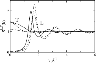
Figure 9: Longitudinal (L) and transverse (T) polarization structure factors of acetonitrile at 298 K. The solid lines refer to the results of MD simulations. Dashed lines indicate the results of PPSF calculations with the input parameters corresponding to ACN3 (Table 5, $m=4.12$ D, $\epsilon_{s}=29.6$, $\epsilon_{\infty}=1.0$) and $\sigma=4.14$ Å. The dash-doted lines indicate the nuclear structure factors $S_{n}^{L,T}(k)$ from the PPSF with the parameters of ambient acetonitrile: $m=3.9$ D, $\epsilon_{s}=35.9$, $\epsilon_{\infty}=1.8$, $\alpha=4.48$ ų, $\eta=0.424$, $\sigma=4.14$ Å.

IV.2 Solute

The solute branch of the calculation algorithm (Fig. 6) consists of the numerical calculation of the Fourier transform of the electric field outside the solute placed in the vacuum. The direct-space electric fields in the initial and final states of the solute are given by a superposition of electric fields produced by partial charges $q_{0k}^{i}$

$$\mathbf{E}_{0i}(\mathbf{r})=\sum_{k=1}^{M_{0}}q_{0k}^{i}\frac{\mathbf{r}-\mathbf{r}_{0k}}{|\mathbf{r}-\mathbf{r}_{0k}|^{3}},$$ (70)

where the sum runs over $M_{0}$ partial charges localized on solute atoms. The field $\mathbf{E}_{0i}(\mathbf{r})$ is Fourier transformed in the region $\Omega$ accessible to the solvent molecules [Eq. (33)]. The region $\Omega$ is generated by assigning vdW radii to all atoms of the solute and then adding the hard sphere radius $\sigma/2$ of the solvent ($\sigma=2.87$ Å for water and 4.14 Å for acetonitrile). This creates the solvent-accessible surface (SAS). The definition of the solute field thus requires atomic coordinates and vdW radii of $N_{0}$ atoms of the solute and $M_{0}$ partial charges $q_{0k}$ to be used in Eq. (70) (indicated as $x_{0k}$, $y_{0k}$, $z_{0k}$, $q_{0k}$ in Fig. 6).

The infinite-space Fourier transform of the Coulomb electric field [Eq. (33)] is numerically divergent Matyushov (2004b). This numerical problem is obviated by splitting the region of integration into the inner part between the SAS and a cutoff sphere and the region outside the cutoff sphere. The Fourier transform within the sphere is calculated numerically by the Fast Fourier Transform (FFT) technique Press et al. (1996) on a cube with the center at the geometrical center of the DSA complex

$$\mathbf{r}_{c}=N_{0}^{-1}\sum_{k=1}^{N_{0}}\mathbf{r}_{0k}.$$ (71)

The length of the cube is chosen by multiplying the maximum extension of the molecule measured from $\mathbf{r}_{c}$ by a factor of 9. This choice yields a sufficiently small increment of the $\mathbf{k}$-grid necessary for the inverted-space integration and, at the same time, avoids numerical errors arising from artificial periodicity imposed by a finite-size numerical FFT technique. The FFT calculation was done on a grid of dimension $256\times 256\times 256$ and the step of 0.5 Å. Calculations on complex 1 involved 143 atoms holding partial charges $q_{0k}^{i}$. The charge shifts ($\Delta q_{k}=q_{0k}^{2}-q_{0k}^{1}$) and coordinates used in the solvent reorganization and free energy calculations are the same as those reported in Ref. Ungar et al., 1999. The individual (i.e., initial and final state) charges used in the reaction free energy calculations are also taken from Ref. Ungar et al., 1999. The field $\mathbf{\tilde{E}}_{0i}(\mathbf{k})$ obtained by combining the numerical and analytical parts is used to calculate the longitudinal and transverse components of the electrostatic energy density in Eqs. (60) and (61). These components are then used in the $k$-integrals with the polarization structure factors (Eqs. (53)–(58); also see Fig. 6).

Table 1: Reorganization energy (kcal/mol) of 1 in water. All calculations except those in the last column are done with $\epsilon_{\infty}=1.0$.

T, K	$\eta$	$y_{p}$	$\epsilon_{s}$	$\lambda_{p}$	$\lambda_{p}$	$\lambda_{p}$	$\lambda_{pq}$	$\lambda_{q}$	$\lambda_{p}$
288	0.4110	6.44	107.7	64.93	39.60	64.35	1.55	4.37	45.88
293	0.4104	6.32	102.1	64.52	39.58	64.26	1.45	4.33	45.47
298	0.4098	6.21	97.5	64.11	39.56	63.93	1.38	4.25	45.07
303	0.4092	6.09	96.0	63.67	39.55	63.52	1.42	4.13	44.68
308	0.4085	5.99	93.7	63.25	39.54	62.98	1.22	4.14	44.30

V Results and comparison to experiment

V.1 Solvent reorganization energy

The solvent reorganization energy of complex 1 was previously obtained from MD simulations of this complex in TIP3P water Ungar et al. (1999). The permanent dipole moment in this force field is enhanced from the vacuum dipole of 1.87 D to 2.35 D to account for water polarizability. This results in a dielectric constant of $\epsilon_{s}=97.5$ from our simulations, which agrees well with $\epsilon_{s}=97.0$ found in the literature Guillot (2002). Table 1 lists the results of calculations of the reorganization energy with structure factors from the PPSF (column 5) and from MD simulations (column 7). The density of the solvent in the $NVT$ simulations was adjusted at each temperature in order to reproduce the expansivity $\alpha_{p}=2.96\times 10^{-4}$ K^-1 of TIP3P water Paschek (2004). The temperature derivative of the reorganization energy thus gives the constant-pressure reorganization entropy corresponding to conditions normally employed in experiment,

$$S_{\lambda}=-(\partial\lambda_{s}/\partial T)_{P}.$$ (72)

Overall, there is an exceptionally good agreement between the reorganization energies calculated by using the structure factors from PPSF and MD simulations. This is not surprising in view of the very good agreement between the two sets of structure factors shown in Fig. 8.

The PPSF result at 298 K, $\lambda_{s}=64.11$ kcal/mol, also compares well with the direct calculation of the reorganization energy from MD simulations, where the value of 60.9 kcal/mol was reported Ungar et al. (1999). The electrostatic forces in those simulations were cut off at distances greater than 10.1 Å. The cutoff is expected to lower the reorganization energy compared to that of an infinite system. In order to estimate the effect of the interaction cutoff, we have calculated the reorganization energy for a fictitious solute with the distance 10.1 Å added to the radius of each atom exposed to the solvent. This contribution amounts to 7.1 kcal/mol. Column 6 in Table 1 shows the results of calculations when the $k$-dependent polarization structure factors are replaced by their $k=0$ values. The gap in $\lambda_{s}$ values between columns 5 and 6 thus quantifies the contribution of the non-local part of solvent response to the reorganization energy. The last (10) column in Table 1 shows the PPSF calculations using parameters of ambient water. In these calculations, the gas phase dipole moment $m=1.87$ D is renormalized by the polarizability effect to give $m^{\prime}=2.43$ D (Wertheim’s 1-RPT formalism Wertheim (1979); Gupta and Matyushov (2004)). Despite this renormalization, $\lambda_{s}$ in this calculation is substantially ($\simeq$ 30 %) smaller than in the calculations using parameters of TIP3P water. TIP3P water thus appears to produce stronger solvation than ambient water.

Table 2: Reorganization energy (kcal/mol) and reorganization entropy (e.u., cal K^-1mol^-1) at T=298 K of complex 1 (experimental parameters for ambient water) calculated with the PPSF for the structure factors.

$\epsilon_{\infty}$	$\epsilon_{s}$	$\lambda_{s}$	$S_{\lambda}$	$\lambda_{s}$	$S_{\lambda}$	$\lambda_{s}$	$\lambda_{s}$
1.0	78.0	52.97	46.50	39.49	$-8.14$	81.12	43.64
1.2	78.0	48.84	52.17	32.84	$-4.85$	69.61	37.44
1.4	78.0	46.41	61.52	28.11	$-2.88$	61.39	33.01
1.6	78.0	45.32	70.66	24.52	$-1.60$	55.23	29.69
1.8	78.00	45.15	80.01	21.74	$-0.71$	50.44	27.11
2.0	78.0	45.68	90.12	19.52	$-0.15$	46.60	26.05
1.0	97.5	64.11	84.13	39.56	2.96	81.44	43.79

Table 1 also presents two components of the solvent reorganization energy produced by solvent quadrupoles: $\lambda_{q}$ is the second cumulant of the coupling of the solute electric field gradient to solvent quadrupole moment Matyushov and Voth (1999); Milischuk and Matyushov (2005a) whereas $\lambda_{pq}$ is a mixed term arising from correlated fluctuations of dipoles and quadrupoles positioned at different solvent molecules Matyushov and Voth (1999); Milischuk and Matyushov (2005c). The resulting solvent reorganization energy is the sum of the dipolar component $\lambda_{p}$ and two quadrupolar components:

$$\lambda_{s}=\lambda_{p}+\lambda_{pq}+\lambda_{q}.$$ (73)

The problem of quadrupolar solvent reorganization has recently attracted much attention Perng et al. (1996a, b); Matyushov and Voth (1999); Jeon and Kim (2001) in connection with new experimental data showing appreciable solvent reorganization in non-dipolar solvents Britt et al. (1995); Reynolds et al. (1996); Kulinowski et al. (1995); Khajehpour and Kauffman (2000); Read et al. (2000). However, the components $\lambda_{q}$ and $\lambda_{pq}$ constitute only a small fraction of the overall reorganization energy despite a relatively high reduced quadrupole of water, $\beta Q^{2}/\sigma^{5}=1.1$ (cf. to $(Q^{*})^{2}=0.13$ of acetonitrile). For the rest of the paper we will therefore assume

$$\lambda_{s}\simeq\lambda_{p}.$$ (74)

We note that the value $\lambda_{s}=69.7$ kcal/mol calculated for TIP3P water with the account of water quadrupoles is in remarkable agreement with $\lambda_{s}=68$ kcal/mol obtained by correcting the simulated values Ungar et al. (1999) by the finite-size cutoff effects.

The dependence of $\lambda_{s}$ and the reorganization entropy on $\epsilon_{\infty}$ are given in Table 2. In these calculations, the vacuum dipole moment of water, 1.83 D, was held constant along with the total dielectric constant $\epsilon_{s}=78.0$. The change in $\epsilon_{\infty}$ was achieved by varying the polarizability $\alpha$ according to the Clausius-Mossotti equation

$$\frac{\epsilon_{\infty}-1}{\epsilon_{\infty}+2}=8\eta\alpha/\sigma^{3},$$ (75)

where $\eta=(\pi/6)\rho\sigma^{3}$ is the solvent packing fraction.

Two drastically different predictions for the effect of solvent polarizability on $\lambda_{s}$ can be found in the literature. The classical Marcus two-sphere model Marcus (1993) predicts a drop of $\lambda_{s}$ by about a factor of 0.6 when going from $\epsilon_{\infty}=1.0$ to $\epsilon_{\infty}=1.8$. On the other hand, simulations using non-polarizable and polarizable versions of the water force field predict almost no dependence of $\lambda_{s}$ on solvent polarizability Bader and Berne (1996); com (d). The actual situation is in between of the two extremes. The reorganization energy does drop with increasing $\epsilon_{\infty}$, but not as much as is predicted by continuum models Gupta and Matyushov (2004). On the other hand, the change is sufficient to make simulations based on non-polarizable solvent models unreliable.

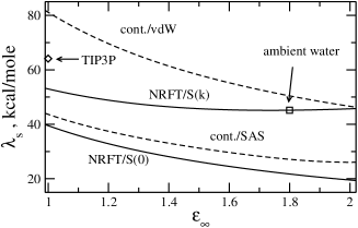
Figure 10: $\lambda_{p}$ vs $\epsilon_{\infty}$ calculated for complex 1 by using the nonlocal polarization response theory (NRFT, solid lines). The dashed lines refer to the numerical solution of the Poisson equation with the vdW (cont./vdW) and SAS (cont./SAS) cavities. The diamond and square indicate TIP3P and ambient water, respectively.

The situation for the dependence of $\lambda_{s}$ on $\epsilon_{\infty}$ is illustrated in Fig. 10, where continuum results for complex 1 obtained with the DelPhi Poisson-Boltzmann solver Rocchia et al. (2002) are compared to the calculations within the NRFT. The dielectric calculations with the vdW dielectric cavity (denoted “cont./vdW” in Fig. 10) show a substantial drop of $\lambda_{s}$ with $\epsilon_{\infty}$. The dependence on $\epsilon_{\infty}$ is much weaker in the NRFT (see also Table 2). The weak dependence of $\lambda_{s}$ on $\epsilon_{\infty}$ is the result of the cancellation of two competing factors: the decrease of the longitudinal structure factor in the range of small $k$-values with increasing $\epsilon_{\infty}$ (Fig. 5) compensated by an increase in $y_{p}$ due to higher solvent dipole $m^{\prime}$ in more polarizable solvents. We note that this cancellation is strongly affected by the $k$-dependence of the polarization structure factors in the range of small $k$-values contributing to the $k$-integral and cannot be reduced to the cancellation of the $y_{p}$ factor in $\lambda_{s}$ [Eqs. (53) and (57)] with $y_{p}$ in the denominator in Eq. (47), resulting in the Pekar factor of continuum electrostatics.

The continuum limit of the NRFT is obtained when the dependence on the wavevector $k$ is neglected in the solvent structure factors and one assumes $S^{L,T}(k)\simeq S^{L,T}(0)$ and $S^{L,T}_{n}(k)\simeq S^{L,T}_{n}(0)$. When this assumption is incorporated in the microscopic calculations (marked NRFT/$S(0)$ in Fig. 10), the resultant reorganization energy gains the strong dependence on $\epsilon_{\infty}$ characteristic of continuum theories. The continuum limit of the microscopic theory corresponds, however, to the dielectric cavity coinciding with the SAS. The corresponding DelPhi calculation (marked cont./SAS in Fig. 10) indeed goes parallel with the continuum limit of the NRFT. The distinction between these two results arises from the mean-field approximation used in the NRFT formulation and different handling of the polarizability effects in the two formulations (additive in the continuum and non-additive in the microscopic formulation Milischuk and Matyushov (2005b)). Note that the mean-field approximation is more accurate, when compared to the exact solution of the Li-Kardar-Chandler equation, in the full microscopic formulation than in its continuum limit Matyushov (2004b). The exact formulation of the theory, which does not involve the mean-field approximation, gives the solution of the Poisson equation in its continuum limit.

The numerical values for the reorganization energies shown in Fig. 10 are given in Table 2. The comparison between the microscopic and continuum calculations is instructive. At $\epsilon_{\infty}=1$, $\lambda_{s}$ from the vdW continuum is much higher than the microscopic calculation, while $\lambda_{s}$ from the SAS continuum is close to the microscopic result. With increasing $\epsilon_{\infty}$, on the other hand, $\lambda_{s}$ from the vdW continuum falls down almost to the microscopic value. The continuum calculation with the vdW cavity may thus appear in a reasonable accord with microscopic calculations or experiment due to the mutual cancellation of errors.

Along with reorganization energies, Table 2 lists reorganization entropies $S_{\lambda}$ [Eq. (72)]. Note that $S_{\lambda}$ obtained from the PPSF calibrated on TIP3P water is in a reasonable agreement with the corresponding value obtained with the structure factors from MD simulations: 84.1 e.u. and 69.9 e.u., respectively. The dielectric continuum calculation gives the wrong sign for the entropy in accord with previous reports Matyushov (1993); Vath et al. (1999). Also the magnitude of $S_{\lambda}$ is substantially higher in the microscopic theory than in the continuum calculation (cf. columns 4 and 6 in Table 2).

A similar trend is seen for the reaction free energy gap (Table 3) for which the reaction entropy is defined as

$$\Delta S_{s}=-\left(\partial\Delta G_{s}/\partial T\right)_{P}.$$ (76)

Although the sign of $\Delta S_{s}$ is correct in the continuum calculations, the entropy magnitude is much lower than in the NRFT, similar to a previous report for a different ET system Vath et al. (1999), where $\Delta S_{s}$ was experimentally obtained from temperature dependent absorption and emission charge-transfer bands. Since the analytical theory seems to be consistent with the computer experiment, one needs a test against experimental data. Unfortunately, experimental evidence on the solvent entropic effects on ET reactions is very limited (see Ref. Zimmt and Waldeck, 2003 for a recent review).

Table 3: Solvation Gibbs energy (kcal/mol) and solvation entropy (e.u., cal K^-1mol^-1).

$\epsilon_{\infty}$	$G_{s,1}$	$S_{s,1}$	$G_{s,2}$	$S_{s,2}$	$\Delta G_{s}$	$\Delta S_{s}$
1.0	$-236.01$	$-198.30$	$-183.36$	$-132.68$	52.65	65.62
1.2	$-245.13$	$-228.90$	$-189.28$	$-151.94$	55.85	76.96
1.4	$-255.10$	$-262.71$	$-195.75$	$-173.15$	59.35	89.56
1.6	$-266.00$	$-299.28$	$-202.79$	$-195.60$	63.21	103.68
1.8	$-277.88$	$-337.52$	$-210.43$	$-219.15$	67.45	118.37
2.0	$-290.77$	$-378.20$	$-218.66$	$-243.41$	72.11	134.79
1.8	$-325.1$	$-2.9$	$-242.1$	$-2.0$	83.0	1.1
1.8	$-196.0$	$-1.46$	$-277.88$	$-1.21$	67.45	0.26

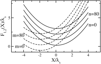
Figure 11: Diabatic initial (solid lines) and final (dashed lines) curves obtained from Eq. (21) for parameters of DSA 1. Curves marked with $n$ and $m$ indexes refer to vibrational states of the initial and final states, respectively. Relative energies are drawn to scale, based on $\lambda_{s}$=45.15 kcal/mol, $\Delta G=-41.2$ kcal/mol, $\hbar\omega_{v}$=400 cm^-1.

V.2 ET rate constant

The calculations of the temperature dependent reorganization energy and equilibrium energy gap can be compared to experimental Arrhenius law measurements Ogawa et al. (1993) for complex 1. Transition metal-based charge-transfer complexes are commonly characterized by metal-ligand vibrational frequencies Ungar et al. (1999) in the range $\omega_{v}\simeq 300-500$ cm^-1, substantially lower than frequencies $\omega_{v}\simeq 1100-1500$ cm^-1 normally assigned to C$-$C skeletal vibrations of organic donor-acceptor complexes. Therefore, Eqs. (1), (2), and (21) with the full quantum-mechanical description of vibrations and temperature-induced populations of vibrational states should be used for the ET rate in complex 1. Unfortunately, our calculations provide only the solvent component of the free energy gap. Its gas-phase component is unknown and the electronic coupling entering the Golden Rule ET rate in Eq. (1) is known with uncertainty Ungar et al. (1999). These two parameters ($\Delta G_{g}$ and $V_{12}$) were varied in fitting the experimental activation enthalpy $\Delta H^{{\dagger}}=9.5$ kcal/mol and the experimental activation entropy $\Delta S^{{\dagger}}/k_{\text{B}}=-5.6$ e.u. Ogawa et al. (1993). Note that the experimental quantity is an effective entropy, including contributions due to the electronic coupling element as well as solvation and inner-sphere vibrational modes Ungar et al. (1999). The Arrhenius analysis was performed by the linear regression of $\ln(k_{ET}/T)$ vs $1/T$ based on the transition-state expression

$$k_{\text{ET}}=\frac{k_{\text{B}}T}{h}e^{-\Delta G^{{\dagger}}(T)/k_{\text{B}}T}.$$ (77)

The rate constant was calculated based on Eqs. (1) and (21), with $\lambda_{s}$ and $\Delta G_{s}$ varied linearly with temperature using the calculated entropies (Tables 2 and 3). The results of calculations are listed in Table 4. The fitted electronic coupling $V_{12}$ falls in the range of values given by electronic structure calculations Ungar et al. (1999) using the semiempirical INDO/s model by Zerner and co-workers Zerner et al. (1980). The equilibrium gap obtained from the fit is appreciably more negative than $\Delta G\simeq-25.4$ kcal/mol estimated from the redox potentials of separate donor and acceptor sites, based on the high spin ground state of the Co²⁺ product (it has been argued Ungar et al. (1999) that the less exothermic low spin Co²⁺ product may be the relevant one in the experimentally observed process). Neglecting the vibrational excitations in the analysis (0-0 transition only) results in a much lower activation enthalpy and a substantially more negative activation entropy (second row in Table 4).

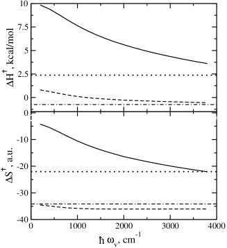
Figure 12: Enthalpy and entropy of activation of DSA complex 1 vs $\hbar\omega_{v}$. The solid lines indicate the calculations according to Eq. (21) with $\lambda_{s}$ and $\Delta G_{s}$ varying linearly with temperature based on the corresponding entropies from Tables 2 and 3. The dashed line indicate the same calculation with $\lambda_{s}$ and $\Delta G_{s}$ fixed at their 298 K values. The dash-dotted ($S_{\lambda}=0$, $\Delta S_{s}=0$) and dotted ($S_{\lambda}\neq 0$, $\Delta S_{s}\neq 0$) lines for the activation enthalpy and entropy refer to the $\omega_{v}\to\infty$ limit corresponding to Eq. (13) with $\lambda_{v}=0$ (no vibrational excitations).

The relatively low frequency of metal-ligand vibrations in transition metal complexes results in a dense manifold of vibrational levels (Fig. 11) which are partially populated at room temperature. The change of the vibrational populations with temperature may result in a contribution to the overall activation entropy Brunschwig et al. (1980). This, however, does not happen for complex 1 when $\lambda_{s}$ and $\Delta G_{s}$ are fixed at their 298 K values. The dashed lines in Fig. 12 show the enthalpy and entropy of activation as a function of the vibrational frequency at constant temperature and $\lambda_{v}$. Increasing the vibrational frequency makes vibrational excitations less accessible, but this is seen to have little effect on the activation entropy and enthalpy.

This situation changes when the temperature dependence of $\lambda_{s}$ and $\Delta G_{s}$ is included in the calculations of the Arrhenius activation parameters. In this case, the temperature dependence of the ET energy gap results in a change of the vibrational quantum numbers corresponding to the maximum vibronic contribution. The splitting of the activation barrier into the entropic and enthalpic contribution then becomes sensitive to the choice of $\omega_{v}$ (Fig. 12, solid lines). This sensitivity may be important for the interpretation of experimental data since the correct definition of the effective vibrational frequency [Eq. (15)] increases in importance once the temperature dependence of the solvation parameters is introduced into the analysis of reaction rates. The classical Marcus-Hush equation with $\lambda_{v}=0$ replaces the sum over all possible vibronic transitions with a single 0-0 transition. The result is a significantly lower enthalpy and more negative entropy of activation (Table 4).

Table 4: Parameters for complex 1 at T=298 K.

Level	$V_{12}$	$\Delta G$	$\hbar\omega_{v}$	$\lambda_{v}$	$\Delta S^{{\dagger}}$	$\Delta H^{{\dagger}}$
	cm-1	kcal/mol	cm-1	kcal/mol	e.u.	kcal/mol
Full	0.07	$-41.2$	400	16.1	$-5.5$	9.4
$\lambda_{v}=0$	0.07	$-25.4$	–	0.0	$-25.0$	2.0

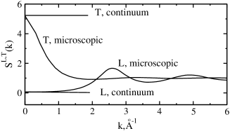
Figure 13: Microscopic structure factors and their continuum limits.

VI Discussion

The most relevant question in comparing microscopic solvation theories with the dielectric continuum approximation is why the latter has allowed to describe so many systems after proper parameterization of dielectric cavities, despite drastic approximations involved. The microscopic NRFT formulation contains dielectric continuum as its limit, allowing us to address this question. The continuum limit is obtained by neglecting the spatial correlations between solvent dipoles, i.e. by neglecting the $k$-dependence in the polarization response functions. This implies that polarization structure factors are replaced by their $k=0$ values (Fig. 13). This replacement is not a good approximation for the transverse structure factor, which changes quite sharply even for small $k$-values, but may be a reasonable approximation for the longitudinal structure factor, which is relatively flat in the range of $k$-values significant for solvation thermodynamics. However, for most charge configurations, even for the point dipole Matyushov (2004a), the contribution of transverse polarization to the solvation free energy is relatively small Matyushov (2004b) ($\simeq 10$% in our calculations for complex 1 in water). Therefore, the inaccurate continuum approximation for the transverse structure factor does not significantly affect the results of calculations.

The continuum estimates for the polarization structure factors result in the following inequalities between the continuum and microscopic longitudinal and transverse components of the reorganization energy

$$\lambda_{s}^{L,\text{cont}}<\lambda_{s}^{L},\quad\lambda_{s}^{T,\text{cont}}>\lambda_{s}^{T}.$$ (78)

The sharp change of the transverse structure factor at small $k$-values is responsible for a substantial overestimate of the transverse component of solvation by continuum models Matyushov (2004a, b). This overestimate manifests itself in solvation dynamics. The transverse polarization dynamics is much slower than the longitudinal polarization dynamics Bagchi and Chandra (1991). Therefore, continuum models predict biphasic solvation dynamics with an appreciable slow component due to transverse polarization relaxation. This slow component is not observed in computer simulations of solvation dynamics Kumar and Maroncelli (1995) and it does not show up in the microscopic calculations reported in Ref. Matyushov, 2005.

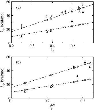
Figure 14: Reorganization energies in polar solvents vs the Pekar factor [Eq. (48)] (a) and the Lippert-Mataga polarity parameter [Eq. (79)] (b). The open points indicate the DelPhi calculations with vdW (squares) and SAS (circles) molecular surfaces. The closed points (triangles) refer to calculations with the NRFT. Numbers on the plot indicate: chloroform (1), tetrahydrofuran (2), methylacetate (3), N,N-dimethylformamide (4), acetone (5), acetonitrile (6), water (7).

The relatively flat form of the longitudinal structure factors at low $k$-values does not mean that replacing $S^{L,T}(k)$ by $S^{L,T}(0)$ gives accurate numbers for the solvation free energy and/or the reorganization energy. A moderate increase of $S^{L}(k)$ in the range of wavevectors contributing to the $k$-integral substantially affects the calculated values of solvation free energies (cf. columns 5 and 6 in Table 1). Moreover, the gap between the microscopic and continuum values changes with the solvent dielectric parameters (see, e.g., Fig. 10). This observation practically means that there is fundamentally no unique scheme for defining the dielectric cavity applicable to all solvent polarities.

The dominance of longitudinal polarization fluctuations in solvation thermodynamics is also responsible for experimentally observed linear trends of the reorganization energy with the Pekar factor Powers and Meyer (1980); Grampp and Jaenicke (1984); Hupp et al. (1993) [Eq. (48)]. Even at the continuum level, the polarization response function for a solute of complex shape is not represented by the Pekar factor appearing in the longitudinal projection of the solvent response function Brunschwig et al. (1986). However, large separation of charges is responsible for the predominantly longitudinal response of the solvent, and continuum reorganization energies calculated for complex 1 in polar solvents correlate well with the Pekar factor (Fig. 14a). If fact, an equally good correlation is seen in respect to the Lippert-Mataga polarity parameter commonly used for solvation of dipoles (Fig. 14b):

$$f_{n}^{\text{LM}}=\frac{\epsilon_{s}-1}{2\epsilon_{s}+1}-\frac{\epsilon_{\infty}-1}{2\epsilon_{\infty}+1}.$$ (79)

The use of a particular parameter does not therefore tell much about the nature of the solute charge distribution and, obviously, reflects a linear relation between $c_{0}$ and $f_{n}^{\text{LM}}$ for common solvents.

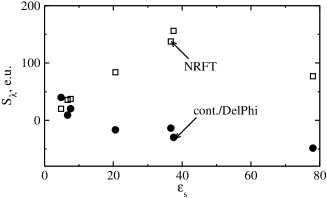
Figure 15: Reorganization entropies from continuum calculations (DelPhi Rocchia et al. (2001) with the vdW surface, closed circles) and by the NRFT (open squares). Points refer to the same solvents as in Fig. 14.

The results of the current microscopic calculations are shown by triangles in Fig. 14. These numbers do not exhibit a linear dependence, although the extent of scatter is not uncommon for ET experiment. The comparison of the continuum and microscopic dependence on the solvent polarity does not permit a clear distinction between the two formulations. Where the distinction becomes clear is for the reorganization entropy in strongly polar solvents. Figure 15 shows reorganization entropies $S_{\lambda}$ calculated in continuum (DelPhi Rocchia et al. (2001) Poisson-Bolzmann solver) and microscopic (NRFT) theories. The continuum calculation reflects the temperature variation of the Pekar factor $c_{0}$:

$$-(\partial c_{0}/\partial T)_{P}=\epsilon_{\infty}^{-2}(\partial\epsilon_{\infty}/\partial T)_{P}-\epsilon_{s}^{-2}(\partial\epsilon_{s}/\partial T)_{P}$$ (80)

In low-polarity solvents, $c_{0}$ is mostly influenced by the static dielectric constant, which has a negative temperature derivative. The continuum reorganization entropy (closed circles in Fig. 15) is positive and is close to the microscopic result (open squares in Fig. 15). The continuum estimate of the temperature variation of $\lambda_{s}$ in low-polarity solvents thus gives a semi-quantitative account of the experimental observations Liang et al. (1989). In strongly polar solvents, the temperature derivative of $c_{0}$ is mostly influenced by the high-frequency dielectric constant, and continuum $S_{\lambda}$ is nagative. In this case, the predictions of the continuum model significantly depart from both the microscopic calculations and many experimental measurements Grampp and Jaenicke (1984); Elliott et al. (1998); Nelsen et al. (1999); Derr and Elliott (1999); Vath et al. (1999); Vath and Zimmt (2000); Zhao et al. (2001), showing positive reorganization entropies.

The microscopic calculations presented here show a relatively weak dependence of the reorganization energy on the solvent high-frequency dielectric constant, in qualitative accord with available computer simulation data Bader and Berne (1996); Ando (2001); Gupta and Matyushov (2004). Testing this theoretical prediction experimentally may become problematic because of the narrow range of $\epsilon_{\infty}$ values available for common polar solvents. We note, however, that the problem of the weak dependence of the reorganization energy on $\epsilon_{\infty}$ is related to the problem of correct sign of the reorganization entropy. The strong dependence of the continuum reorganization energy on $\epsilon_{\infty}$ is one of major factors shifting the continuum reorganization entropy to the range of positive values.

The calculations of the quadrupolar component of the solvent reorganization energy presented here confirm the conclusion previously reached for Stokes shifts in coumarin-153 optical dye Matyushov and Newton (2001): quadrupolar solvation is insignificant in most commonly used polar solvents, and the dipolar approximation for the solvent charge distribution is sufficient for most practical calculations.

Appendix A Simulation and analysis.

The MC simulations of dipolar-polarizable hard sphere solvents shown in Fig. 7 were done as described in Ref. Gupta and Matyushov, 2004. Simulations of $6\times 10^{5}$ cycles long were run for 1372 polarizable molecules with periodic boundary conditions and the reaction field cutoff of dipole-dipole interactions. The MD simulations were carried out with the force field of 3-site acetonitrile (ACN3) by Edwards, Madden, and McDonald Edwards et al. (1984) and the 3-site model of water (TIP3P) by Jorgensen et al. Jorgensen et al. (1983) (Table 5). The site-site interaction potential is given by the sum of the Lennard-Jones (LJ) and Coulomb interaction potentials:

$$E_{\alpha\beta}=4\varepsilon_{\alpha\beta}\left[\left(\dfrac{\sigma_{\alpha\beta}}{r_{\alpha\beta}}\right)^{12}-\left(\dfrac{\sigma_{\alpha\beta}}{r_{\alpha\beta}}\right)^{6}\right]+\dfrac{q_{\alpha}q_{\beta}}{r_{\alpha\beta}},$$ (81)

where the LJ parameters are taken according to the Lorentz-Bertholet rules: $\varepsilon_{\alpha\beta}=\sqrt{\varepsilon_{\alpha}\varepsilon_{\beta}}$ and $\sigma_{\alpha\beta}=(\sigma_{\alpha}+\sigma_{\beta})/2$. All simulations were done with the DL_POLY molecular dynamics package Smith and Forester (1996). We run two sets of MD simulations in the temperature range from 288 K to 308 K with a 5 K step. The timestep in each simulation is 5 fs. All MD simulation are 20 ns long.

Table 5: Force field parameters for use in the simulation.

Atomic interaction site	$\sigma_{\alpha}$/Å	$\varepsilon_{\alpha}\times 10^{3}$/ (kcal/mol)	$q_{\alpha}$/ e
TIP3P water
O	3.15	152.10	$-0.834$
Acetonitrile
Me	3.6	379.55	0.269
C	3.4	99.36	0.129
N	3.3	99.36	$-0.398$

We used the Nosé-Hoover thermostat Hoover (1985) for the ACN3 simulations with the relaxation parameter of 0.5 fs. This value ensures good stabilization of the total system energy. The energy drift for ACN3 is only about 0.1%. The simulation box was constructed to include 256 ACN3 molecules in a cube with the side length $L=28.2025$ Å at T=298 K to reproduce the experimental mass density of acetonitrile, $\rho_{M}$=0.777 g/cm³. The side length is adjusted at each temperature to account for temperature expansion with the experimental volume expansion coefficient $\alpha_{p}=1.38\times 10^{-3}$ K^-1.

In simulations of TIP3P water, 256 molecules reside in a cube with the side length of $L=19.7744$ Å at 298 K. The system is coupled to the Berendsen Berendsen et al. (1984) thermostat with the relaxation time of 0.1 fs. The drift in total energy of about 0.1 % is observed. The liquid mass density $\rho_{M}=0.9896$ g/cm³ and the volume expansion coefficient $\alpha_{p}=2.96\times 10^{-3}$ K^-1 are taken from Ref. Paschek, 2004. The latter value is close to the experimental expansion coefficient of ambient water, $\alpha_{p}=2.6\times 10^{-3}$ K^-1.

The cutoff for short-range LJ interaction is 13 Å for ACN3 and 9 Å for TIP3P. For long-range Coulomb interactions, Ewald summation from DL_POLY Allen and Tildesley (1996) is used for ACN3 and smoothed particle mesh (SPME) Essmann et al. (1995) Ewald is adopted for TIP3P. Ewald summation parameters are the convergence parameter $\alpha$ and the maximum wavenumber $k^{max}_{x,y,z}$. The parameter sets $\alpha=0.24$ Å^-1, $k^{max}_{x,y,z}=7$ Å^-1, and $\alpha$ =0.35 Å^-1, ${k}^{max}_{x,y,z}=8$ Å^-1 were used for ACN3 and TIP3P respectively.

The structure factors have been calculated as the variance of longitudinal and transverse projections of the $\mathbf{k}$-space solvent polarization

$$\mathbf{M}(k)=(1/m)\sum_{i=1}^{N}\mathbf{m}_{i}e^{-\mathit{i}\mathbf{k}\cdot\mathbf{r}_{i}},$$ (82)

where $\mathbf{m}_{i}=\sum_{a}q_{a}\mathbf{r}_{i}^{a}$ is a dipole moment of the $i$th molecule and the sum runs over the $N$ molecules in the simulation box. The static dielectric constant is given in terms of the $k=0$ variance as follows Neumann (1986)

$$\varepsilon_{s}=1+3y\langle\mathbf{M(0)}^{2}\rangle/N,$$ (83)

where $y=(4\pi/9)\rho m^{2}/k_{\text{B}}T$.

References

- Marcus (1993) R. A. Marcus, Rev. Mod. Phys. 65, 599 (1993).
- Marcus and Sutin (1985) R. A. Marcus and N. Sutin, Biochim. Biophys. Acta 811, 265 (1985).
- Winkler and Gray (1992) J. R. Winkler and H. B. Gray, Chem. Rev. 92, 369 (1992).
- McLendon and Hake (1992) G. McLendon and R. Hake, Chem. Rev. 92, 481 (1992).
- Warshel (2002) A. Warshel, Acc. Chem. Res. 35, 385 (2002).
- Gregory (1995) R. B. Gregory, in Protein-solvent interactions, edited by R. B. Gregory (Marcel Dekker, New York, 1995), p. 191.
- Rocchia et al. (2001) W. Rocchia, E. Alexov, and B. Honig, J. Phys. Chem. B 105, 6507 (2001).
- Siriwong et al. (2003) K. Siriwong, A. A. Voityuk, M. D. Newton, and N. Rösch, J. Phys. Chem. B 107, 2595 (2003).
- Roux et al. (1990) B. Roux, H.-A. Yu, and M. Karplus, J. Phys. Chem. 94, 4683 (1990).
- Lynden-Bell (1999) R. M. Lynden-Bell, in Simulation and theory of electrostatic interactions in solution (American Institute of Physics, Melville, New York, 1999), AIP Conference proceedings, p. 3.
- Rick and Berne (1994) S. W. Rick and B. J. Berne, J. Am. Chem. Soc. 116, 3949 (1994).
- Vath et al. (1999) P. Vath, M. B. Zimmt, D. V. Matyushov, and G. A. Voth, J. Phys. Chem. B 103, 9130 (1999).
- Lee and Hynes (1988) S. Lee and J. T. Hynes, J. Chem. Phys. 88, 6853 (1988).
- Kuznetsov (1992) A. M. Kuznetsov, J. Phys. Chem. 96, 3337 (1992).
- Gehlen et al. (1992) J. N. Gehlen, D. Chandler, H. J. Kim, and J. T. Hynes, J. Phys. Chem. 96, 1748 (1992).
- Zhu and Cukier (1995) J. Zhu and R. I. Cukier, J. Chem. Phys. 102, 8398 (1995).
- Bader and Berne (1996) J. S. Bader and B. J. Berne, J. Chem. Phys. 104, 1293 (1996).
- Ando (2001) K. Ando, J. Chem. Phys. 115, 5228 (2001).
- Gupta and Matyushov (2004) S. Gupta and D. V. Matyushov, J. Phys. Chem. A 108, 2087 (2004).
- Marchi et al. (2001) M. Marchi, D. Borgis, N. Vevy, and P. Ballone, J. Chem. Phys. 114, 4377 (2001).
- Leontyev et al. (2003) I. V. Leontyev, M. V. Vener, I. V. Rostov, M. V. Basilevsky, and M. D. Newton, J. Chem. Phys. 119, 8024 (2003).
- Raineri and Friedman (1999) F. O. Raineri and H. L. Friedman, Adv. Chem. Phys. 107, 81 (1999).
- Beglov and Roux (1996) D. Beglov and B. Roux, J. Chem. Phys. 104, 8678 (1996).
- Kornyshev (1985) A. A. Kornyshev, in The Chemical Physics of Solvation, edited by R. R. Dogonadze, E. Kálman, A. A. Kornyshev, and J. Ulstrup (Elsevier, 1985), vol. A, p. 77.
- Kornyshev and Ulstrup (1986) A. A. Kornyshev and J. Ulstrup, Chem. Phys. Lett. 126, 74 (1986).
- Fried and Mukamel (1990) L. E. Fried and S. Mukamel, J. Chem. Phys. 93, 932 (1990).
- Bagchi and Chandra (1991) B. Bagchi and A. Chandra, Adv. Chem. Phys. 80, 1 (1991).
- Chandler (1993) D. Chandler, Phys. Rev. E 48, 2898 (1993).
- Matyushov (1993) D. V. Matyushov, Chem. Phys. 174, 199 (1993).
- Song et al. (1996) X. Song, D. Chandler, and R. A. Marcus, J. Phys. Chem. 100, 11954 (1996).
- Kornyshev and Sutmann (1996) A. A. Kornyshev and G. Sutmann, J. Chem. Phys. 104, 1524 (1996).
- Song and Chandler (1998) X. Song and D. Chandler, J. Chem. Phys. 108, 2594 (1998).
- Lang et al. (1999) M. J. Lang, X. J. Jordanides, X. Song, and G. R. Fleming, J. Chem. Phys. 110, 5884 (1999).
- Ramirez et al. (2002) R. Ramirez, R. Gebauer, M. Mareschal, and D. Borgis, Phys. Rev. E 66, 031206 (2002).
- Matyushov (2004a) D. V. Matyushov, J. Chem. Phys. 120, 1375 (2004a).
- Matyushov (2004b) D. V. Matyushov, J. Chem. Phys. 120, 7532 (2004b).
- LeBard et al. (2003) D. N. LeBard, M. Lilichenko, D. V. Matyushov, Y. A. Berlin, and M. A. Ratner, J. Phys. Chem. B 107, 14509 (2003).
- Milischuk and Matyushov (2005a) A. Milischuk and D. V. Matyushov, J. Chem. Phys. (2005a), in press, cond-mat/0504265.
- Matyushov (2005) D. V. Matyushov, J. Chem. Phys. 122, 044502 (2005).
- Ungar et al. (1999) L. W. Ungar, M. D. Newton, and G. A. Voth, J. Phys. Chem. B 103, 7367 (1999).
- Ogawa et al. (1993) M. Y. Ogawa, J. F. Wishart, Z. Young, J. R. Miller, and S. S. Isied, J. Phys. Chem. 97, 11456 (1993).
- Dong and Hupp (1992) Y. Dong and J. T. Hupp, Inorg. Chem. 31, 3322 (1992).
- Elliott et al. (1998) C. M. Elliott, D. L. Derr, D. V. Matyushov, and M. D. Newton, J. Am. Chem. Soc. 120, 11714 (1998).
- Nelsen et al. (1999) S. F. Nelsen, R. F. Ismagilov, K. E. Gentile, and D. R. Powell, J. Am. Chem. Soc. 121, 7108 (1999).
- Derr and Elliott (1999) D. L. Derr and C. M. Elliott, J. Phys. Chem. A 103, 7888 (1999).
- Vath and Zimmt (2000) P. Vath and M. B. Zimmt, J. Phys. Chem. A 104, 2626 (2000).
- Zhao et al. (2001) X. Zhao, J. A. Burt, F. J. Knorr, and J. L. McHale, J. Phys. Chem. A 105, 11110 (2001).
- Coropceanu et al. (2003) V. Coropceanu, C. Lambert, G. Nöll, and J. L. Brédas, Chem. Phys. Lett. 373, 153 (2003).
- Mertz (2005) E. L. Mertz, J. Phys. Chem. A 109, 44 (2005).
- Grampp and Jaenicke (1984) G. Grampp and W. Jaenicke, Ber. Bunsenges. Phys. Chem. 88, 335 (1984), this paper does not directly report the slope of the reorganization energy vs temperature. The negative slope can be, however, extracted by combining the dependence of the rate on the Pekar factor with the rate temperature dependence.
- Liang et al. (1989) N. Liang, J. R. Miller, and G. L. Closs, J. Am. Chem. Soc. 111, 8740 (1989), the negative slope of the reorganization energy vs temperature in a weakly polar solvent is obtained in this paper from the dielectric continuum estimate. The temperature correction of the solvent reorganization energy describes better the observed temperature dependence of the ET rate.
- Leontiev and Basilevskii (2005) I. V. Leontiev and M. V. Basilevskii, Russ. J. Phys. Chem. 79, 419 (2005).
- Kumar et al. (1998) K. Kumar, I. V. Kurnikov, D. N. Beratan, D. H. Waldeck, and M. B. Zimmt, J. Phys. Chem. A 102, 5529 (1998).
- Kubo and Toyozawa (1955) R. Kubo and Y. Toyozawa, Prog. Theor. Phys. 13, 160 (1955).
- Bixon and Jortner (1999) M. Bixon and J. Jortner, Adv. Chem. Phys. 106, 35 (1999).
- Ovchinnikov and Ovchinnikova (1969) A. A. Ovchinnikov and M. Y. Ovchinnikova, JETPh 29, 688 (1969).
- Mukamel (1995) S. Mukamel, Principles of Nonlinear Optical Spectroscopy (Oxford University Press, New York, 1995).
- Holstein (1959) T. Holstein, Ann. Phys. 8, 343 (1959).
- Hopfield (1974) J. J. Hopfield, Proc. Nat. Acad. Sci. 71, 3640 (1974).
- Siders and Marcus (1981) P. Siders and R. A. Marcus, J. Am. Chem. Soc. 103, 741 (1981).
- Marcus (1989) R. A. Marcus, J. Phys. Chem. 93, 3078 (1989).
- Jortner (1976) J. Jortner, J. Chem. Phys. 64, 4860 (1976).
- Lax (1952) M. Lax, J. Chem. Phys. 20, 1752 (1952).
- Davydov (1953) A. C. Davydov, JETPh 24, 397 (1953).
- Perng et al. (1996a) B.-C. Perng, M. D. Newton, F. O. Raineri, and H. L. Friedman, J. Chem. Phys. 104, 7153 (1996a).
- Perng et al. (1996b) B.-C. Perng, M. D. Newton, F. O. Raineri, and H. L. Friedman, J. Chem. Phys. 104, 7177 (1996b).
- Matyushov and Voth (1999) D. V. Matyushov and G. A. Voth, J. Chem. Phys. 111, 3630 (1999).
- com (a) The nuclear polarization also includes atomic polarization due to intramolecular flexibility of the solvent. The influence of these effects is estimated to be relatively minor, see p. 7183 in Ref. Perng et al., 1996b and H. Sumi and R. A. Marcus, J. Chem. Phys. 84 (1986) 4272.
- Matyushov and Ladanyi (1998) D. V. Matyushov and B. M. Ladanyi, J. Chem. Phys. 108, 6362 (1998).
- Madden and Kivelson (1984) P. Madden and D. Kivelson, Adv. Chem. Phys. 56, 467 (1984).
- Hwang and Warshel (1987) J.-K. Hwang and A. Warshel, J. Am. Chem. Soc. 109, 715 (1987).
- Kuharski et al. (1988) R. A. Kuharski, J. S. Bader, D. Chandler, M. Sprik, M. L. Klein, and R. W. Impey, J. Chem. Phys. 89, 3248 (1988).
- Marchi et al. (1993) M. Marchi, J. N. Gehlen, D. Chandler, and M. Newton, J. Am. Chem. Soc. 115, 4178 (1993).
- Yelle and Ichiye (1997) R. B. Yelle and T. Ichiye, J. Phys. Chem. B 101, 4127 (1997).
- Hartnig and Koper (2001) C. Hartnig and M. T. M. Koper, J. Chem. Phys. 115, 8540 (2001).
- Born (1920) M. Born, Z. Phys. 1, 45 (1920).
- Onsager (1936) L. Onsager, J. Am. Chem. Soc. 58, 1486 (1936).
- Li and Kardar (1992) H. Li and M. Kardar, Phys. Rev. A 46, 6490 (1992).
- Raineri et al. (1994) F. O. Raineri, H. Resat, B.-C. Perng, F. Hirata, and H. L. Friedman, J. Chem. Phys. 100, 1477 (1994).
- Matyushov (1996) D. V. Matyushov, Chem. Phys. 211, 47 (1996).
- Kharkats et al. (1976) Y. I. Kharkats, A. A. Kornyshev, and M. A. Vorotyntsev, Faraday Trans. II 72, 361 (1976).
- Kuznetsov and Medvedev (1996) A. M. Kuznetsov and I. G. Medvedev, J. Phys. Chem. 100, 5721 (1996).
- Chandra and Bagchi (1989) A. Chandra and B. Bagchi, J. Phys. Chem. 93, 6996 (1989).
- Bagchi and Chandra (1989) B. Bagchi and A. Chandra, Chem. Phys. Lett. 155, 533 (1989).
- Schaefer and Karplus (1996) M. Schaefer and M. Karplus, J. Phys. Chem. 100, 1578 (1996).
- com (b) Different partitioning schemes of the solvent polarization into the fast and slow components can be implemented for solvation thermodynamics calculations Pekar (1963); Brady and Carr (1985); Aguilar (2001). Although they all give identical results for the thermodynamics of solvation, they will lead to different predictions regarding the solvation dynamics. The Pekar partitioning results in slow relaxation of the component of induced dipole ( in Eq. (37)) in equilibrium with the field of permanent dipoles in the liquid.
- Stell et al. (1981) G. Stell, G. N. Patey, and J. S. Høye, Adv. Chem. Phys. 18, 183 (1981).
- Pekar (1963) S. I. Pekar, Research in electron theory of crystals (USAEC, Washington, D.C., 1963).
- Pekar (1946) S. I. Pekar, JETPh 16, 341 (1946).
- Brady and Carr (1985) J. E. Brady and P. W. Carr, J. Phys. Chem. 89, 5759 (1985).
- Aguilar (2001) M. A. Aguilar, J. Phys. Chem. A 105, 10393 (2001).
- Milischuk and Matyushov (2005b) A. A. Milischuk and D. V. Matyushov, J. Chem. Phys. (2005b), to be submitted.
- Wertheim (1979) M. S. Wertheim, Molec. Phys. 37, 83 (1979).
- Perng and Ladanyi (1999) B.-C. Perng and B. M. Ladanyi, J. Chem. Phys. 110, 6389 (1999).
- Schmid and Matyushov (1995) R. Schmid and D. V. Matyushov, J. Phys. Chem. 99, 2393 (1995).
- Wertheim (1971) M. S. Wertheim, J. Chem. Phys. 55, 4291 (1971).
- Gray and Gubbins (1984) C. G. Gray and K. E. Gubbins, Theory of Molecular Liquids (Clarendon Press, Oxford, 1984).
- Fonseca and Ladanyi (1990) T. Fonseca and B. M. Ladanyi, J. Chem. Phys. 11, 8148 (1990).
- Raineri and Friedman (1993) F. Raineri and H. Friedman, J. Chem. Phys. 98, 8910 (1993).
- Skaf and Ladanyi (1995) M. S. Skaf and B. M. Ladanyi, J. Chem. Phys. 102, 6542 (1995).
- Jorgensen et al. (1983) W. L. Jorgensen, J. Chandrasekhar, J. D. Madura, R. W. Impey, and M. L. Klein, J. Chem. Phys 79, 926 (1983).
- Edwards et al. (1984) D. M. F. Edwards, P. A. Madden, and I. R. McDonald, Mol. Phys 51, 1141 (1984).
- com (c) The quadrupole moment is a tensor; the scalar quadrupole moment is defined as Gray and Gubbins (1984).
- Bopp et al. (1996) P. A. Bopp, A. A. Kornyshev, and G. Sutmann, Phys. Rev. Lett. 76, 1280 (1996).
- Skaf (1997) M. S. Skaf, J. Chem. Phys. 107, 7996 (1997).
- Bopp et al. (1998) P. A. Bopp, A. A. Kornyshev, and G. Sutmann, J. Chem. Phys. 109, 1939 (1998).
- Omelyan (1999) I. P. Omelyan, Mol. Phys. 407, 407 (1999).
- Press et al. (1996) W. H. Press, S. A. Teukolsky, W. T. Vetterling, and B. P. Flannery, Numerical recipes in Fortran 77: The art of scientific computing (Cambridge University Press, 1996).
- Guillot (2002) B. Guillot, J. Mol. Liq. 101, 219 (2002).
- Paschek (2004) D. Paschek, J. Chem. Phys 120, 6674 (2004).
- Milischuk and Matyushov (2005c) A. A. Milischuk and D. V. Matyushov, J. Chem. Phys. (2005c), to be submitted.
- Jeon and Kim (2001) J. Jeon and H. J. Kim, J. Sol. Chem. 30, 849 (2001).
- Britt et al. (1995) B. M. Britt, J. L. McHale, and D. M. Friedrich, J. Phys. Chem. 99, 6347 (1995).
- Reynolds et al. (1996) L. Reynolds, J. A. Gardecki, S. J. V. Frankland, and M. Maroncelli, J. Phys. Chem. 100, 10337 (1996).
- Kulinowski et al. (1995) K. Kulinowski, I. R. Gould, and A. B. Myers, J. Phys. Chem. 99, 9017 (1995).
- Khajehpour and Kauffman (2000) M. Khajehpour and J. F. Kauffman, J. Phys. Chem. A 104, 9512 (2000).
- Read et al. (2000) I. Read, A. Napper, M. B. Zimmt, and D. H. Waldeck, J. Phys. Chem. A 104, 9385 (2000).
- com (d) In the simulations of Bader and Berne Bader and Berne (1996) the charge induced by formaldehyde taken as a solute on each solvent molecule (corresponding to dipole in Eq. (37)) was not subtracted from the overall induced charge. Their reported reorganization energies correspond, therefore, to the sum of the reorganization energy due to nuclear polarization fluctuations, , and a reorganization energy arising from fluctuations of the solute-solvent induction interaction, (see, e.g., D. V. Matyushov and R. Schmid, Mol. Phys. 84, 533 (1995)).
- Rocchia et al. (2002) W. Rocchia, S. Sridharan, A. Nicholls, E. Alexov, A. Chiabrera, and B. Honig, J. Comput. Chem. 23, 128 (2002).
- Zimmt and Waldeck (2003) M. B. Zimmt and D. H. Waldeck, J. Phys. Chem. A 107, 3580 (2003).
- Zerner et al. (1980) M. Zerner, G. H. Loew, R. F. Kirchner, and U. T. Mueller-Westerhoff, J. Am. Chem. Soc. 102, 589 (1980).
- Brunschwig et al. (1980) B. S. Brunschwig, J. Logan, M. D. Newton, and N. Sutin, J. Am. Chem. Soc. 102, 5798 (1980).
- Kumar and Maroncelli (1995) P. V. Kumar and M. Maroncelli, J. Chem. Phys. 103, 3038 (1995).
- Powers and Meyer (1980) M. J. Powers and T. J. Meyer, J. Am. Chem. Soc. 102, 1289 (1980).
- Hupp et al. (1993) J. T. Hupp, Y. Dong, R. L. Blackbourn, and H. Lu, J. Phys. Chem. 97, 3278 (1993).
- Brunschwig et al. (1986) B. S. Brunschwig, S. Ehrenson, and N. Sutin, J. Phys. Chem. 90, 3657 (1986).
- Matyushov and Newton (2001) D. V. Matyushov and M. D. Newton, J. Phys. Chem. A 105, 8516 (2001).
- Smith and Forester (1996) W. Smith and T. R. Forester, J. Molec. Graphics 14, 136 (1996).
- Hoover (1985) W. G. Hoover, Phys. Rev. A 31, 1695 (1985).
- Berendsen et al. (1984) H. J. C. Berendsen, J. P. M. Postma, W. van Bunsteren, A. DiNola, and J. R. Haak, J. Chem. Phys. 81, 3684 (1984).
- Allen and Tildesley (1996) M. P. Allen and D. J. Tildesley, Computer Simulation of Liquids (Clarendon Press, Oxford, 1996).
- Essmann et al. (1995) U. Essmann, L. Perera, M. L. Berkowitz, T. Darden, H. Lee, and L. G. Pedersen, J. Chem. Phys. 103, 8577 (1995).
- Neumann (1986) M. Neumann, Mol. Phys. 57, 97 (1986).