Long range scattering resonances in strong-field seeking states of polar molecules

Abstract

We present first steps toward understanding the ultracold scattering properties of polar molecules in strong electric field-seeking states. We have found that the elastic cross section displays a quasi-regular set of potential resonances as a function of the electric field, which potentially offers intimate details about the inter-molecular interaction. We illustrate these resonances in a “toy” model composed of pure dipoles, and in more physically realistic systems. To analyze these resonances, we use a simple WKB approximation to the eigenphase, which proves both reasonably accurate and meaningful. A general treatment of the Stark effect and dipolar interactions is also presented.

I Introduction

Conventional spectroscopy of atoms and molecules begins with the premise that the energy levels of the species being probed are fixed although they may shift slightly in electromagnetic fields. These levels are then interrogated by energy-dependent probes such as photons or charged or neutral particles. Information on the energetics and structure of the molecules is extracted from absorption energies, oscillator strengths, selection rules, etc. In these investigations, the study of resonances has played a central role.

With the advent of ultracold environments for atoms and molecules, this general view of spectroscopy can be inverted. Cold collisions provide a nearly monochromatic probe of near-threshold intermolecular interactions, with resolution set by the milliKelvin or microKelvin temperature of the gas. In this case the energy levels of nearby resonant states can be tuned into resonance with the zero-energy collisions. For cold gases of alkali atoms, this strategy is already in widespread use. It exploits the fact that the Zeeman effect can shift the internal energies of the atoms over ranges orders of magnitude larger than the collision energy itself. In this way, atoms can be made to resonate when they would not naturally do so (i.e., in zero field). Measurement of these “Feshbach” resonances (more properly, Fano-Feshbach resonances) has yielded the most accurate determination of alkali-alkali potential energy surfaces for near-threshold processes potentials .

The current experimental and theoretical push to create and study ultracold molecules cold-rev will lead to many more opportunities for this novel kind of spectroscopy, since molecules possess many more internal degrees of freedom than do atoms. There will be, for example, numerous Fano-Feshbach resonances in which one or both of the collision partners becomes vibrationally or rotationally excited Forrey ; Deskevich ; Bala ; statistical arguments suggest that these resonances will be quite narrow in energy, a fact related to their abundance Deskevich . A second class of resonant states will occur when the constituents are excited into higher-lying fine structure or hyperfine structure states, more reminiscent of the resonances observed in the alkali atoms. In molecules, these resonances are naturally also tunable in energy using magnetic fields krems .

In this paper, we are primarily interested in a third class of resonance: potential resonances that are engendered by altering the intermolecular potential energy surface itself. This capability becomes especially prominent in cold collisions of heteronuclear polar molecules, whose dipolar interactions are quite strong on the scale of the low translational temperatures of the gas. At the same time, the dipole moments of the individual dipoles can be strengthened or weakened as well as aligned by an applied electric field.

This kind of resonance includes the shape resonances, discussed in the context of cold atoms polarized by strong electric fields shape-you ; Deb . A second set, dubbed “field-linked” resonances, has been studied in some detail in Refs AA_PRL ; AA_PRA ; AA_FL . These states appear in potential energy surfaces (PES’s) that correlate to weak electric field-seeking states of the free molecules. They are weakly bound, long-ranged in character, and indeed do not appear to exist without an electric field present. Similar resonances are predicted to occur in metastable states of the alkaline earth elements at low temperatures derev ; santra .

A rich set of potential resonances emerges among strong-field seeking states, and this is the subject of the present paper. Strong-field seekers are of increasing importance experimentally, since they would enable molecules to be trapped in their absolute ground states where no 2-body inelastic collision processes are available to harm the gas. In this case, the colliding molecules are free to approach to within a small internuclear distance of one another; the resulting potential resonances therefore can probe detailed intermolecular dynamics near threshold. The resulting data, consisting of scattering peaks as a function of electric field, can be thought of as a kind of “Stark spectroscopy”. Just such a tool has been applied previously in precision measurements of alkali Rydberg spectra Ryd1 ; Ryd2 .

In this paper we explore such spectra in ultracold molecules, finding that the spectrum is dominated by a quasi-regular series in the electric field values. Such a series is the fundamental building block of molecular Stark spectroscopy and plays a role analogous to the Rydberg series in atomic spectroscopy. In both cases, the series lays out the fundamental structure of the unperturbed, long-range physics between interacting entities. In the case of atoms, the deviation from an unperturbed Rydberg series, encapsulated in the quantum defects, yields information on the electron-core interaction Seaton ; qdt . Similarly, it is expected that differences in observed Stark spectra from those presented here will probe the short-range intermolecular interactions.

To emphasize the generality of these resonances, we first briefly develop in Sec. II a general formalism for arbitrary polar collision partners, covering explicitly Hund’s cases (a) and (b) as well as asymmetric rotor molecules. Using this formalism, we introduce in Sec. III the potential resonances using a simplified version of the molecular gas in which all dipoles are assumed to be perfectly aligned and where molecular fine structure plays no role. In Sec. IV, we consider the case of more realistic molecules, where fine structure does intervene. We show that the structure of the potential resonances is unchanged, but that additional narrow Fano-Feshbach resonances do appear. Throughout the article we emphasize how the various types of resonance can be classified and organized by simple considerations involving the WKB approximation.

II General Form of the Stark Effect and dipolar interaction

In this section, we briefly recapitulate our scattering model which is presented in Refs.AA_PRA ; CT1 ; CT_thesis . The molecular scattering Hamiltonian can be written as

$$H=T_{0}+V_{SR}+V_{LR}+H_{S}+H_{int}$$ (1)

Where $T_{0}$ is the kinetic energy operator, $V_{SR}$ is the short range potential energy surface (PES), $V_{LR}$ is the long range interaction of the polar molecules, $H_{S}$ is the Stark Hamiltonian, and $H_{int}$ is the Hamiltonian describing the internal degrees of freedom of the molecules. For the purpose of this paper we disregard $V_{SR}$. The long range interaction is dominated by the dipole-dipole interaction AA_PRA . Furthermore an electric field can significantly change the structure of the interaction and be used to control the molecular collisions AA_PRA ; CT1 .

The first step in performing a scattering calculation is to construct a basis of molecular energy eigenstates in an external field. Here we generalize the approach slightly to make it applicable to various types of polar molecules. Once the Stark Hamiltonian is obtained, the result can be used in the Hamiltonian of the dipolar interaction, showing their common physical origin in terms of electric fields.

To simplify the analysis and calculations, we assume that the vibrational degrees of freedom are frozen out at low temperatures; hence can treat the molecules as rigid rotors. The molecular state is described in terms of the state $|JM_{J}\Omega\rangle$, where $J$ is the molecule’s rotational plus electronic angular momenta, $M_{J}$ is the projection of $J$ onto the lab axis, and $\Omega$ is $J$’s projection onto the molecular axis. To describe the rigid rotor molecular wave function, we use $\langle\alpha,\beta,\gamma|JM_{J}\Omega\rangle=\sqrt{2J+1\over 8\pi^{2}}D^{J\star}_{M_{J}\Omega}(\alpha,\beta,\gamma)$, where $\alpha,\beta,$ and $\gamma$ are the Euler angles defining the molecular axis and $D^{J\star}_{M_{J}\Omega}$ is a Wigner D-function Brown .

II.1 The Stark effect

Since the electric field is a true vector (as opposed to a pseudovector), it only couples states of opposite parity. This implies that the Stark energies vary quadratically with low electric field; they vary linearly only at higher fields once the Stark energy is greater than the energy splitting of the two states. The Stark Hamiltonian has the form

$$H_{S}=-{\vec{\mu}}\cdot\vec{\cal E}.$$ (2)

For the current discussion, we pursue a general approach and allow the field to point in any direction in the laboratory reference frame. This general approach allows the matrix elements to be used in the dipolar interaction. However when explicitly considering the molecular states in an electric field, we that the field lies in the $\hat{z}$ direction.

The Stark interaction can be evaluated by decomposing the electric field in spherical coordinates and then rotating the dipole into the lab frame. In this representation, the Stark Hamiltonian has the form $H_{S}=-\sum_{q}\mu{\cal E}D^{1\star}_{q0}$, where $\mu$ is the electric dipole moment of the molecule and $D^{1\star}$ is a Wigner D-function. $D^{1\star}_{q0}$ is equal to $(-1)^{2q}C^{1}_{q}$, a reduced spherical harmonic Brink , and $q$ is the projection quantum number of $\cal E$ onto the lab axis. At the heart of evaluating the Stark effect, we find the operator $D^{1\star}$ coupling two molecular states, which themselves are described by D functions. The Stark matrix element is an integral of three D-functions over the molecular coordinates, averaging over molecular orientation. The evaluation of the integral results in selection rules whose details depend on the molecular specifics. For a valuable qualitative discussion on the Stark effect see Schreel .

A given molecule may also have a nuclear spin that generates a hyperfine structure. In this case, it is more appropriate to present the matrix elements in the hyperfine basis, where $F$ and $M_{F}$ define the state. Here $F$ is the sum of $J$ and the nuclear spin $I$ and $M_{F}$ is the projection of $F$ in the lab frame. We use the Wigner-Eckart theorem to compute the Stark matrix elements in a compact form. The matrix elements of the Stark effect are written as

$$\langle\alpha FM_{F}|H_{S}|\alpha^{\prime}F^{\prime}M_{F}^{\prime}\rangle=-\mu{\cal E}\langle\alpha FM_{F}|D^{1\star}_{q0}|F^{\prime}M_{F}^{\prime}\alpha^{\prime}\rangle,$$ (3)

which contains a purely geometrical matrix element

$$\langle\alpha FM_{F}|D^{1\star}_{q0}|F^{\prime}M_{F}^{\prime}\alpha^{\prime}\rangle=[F](-1)^{1+M_{F}+F^{\prime}}$$

$$\times\left(\begin{array}[]{ccc}F^{\prime}&1&F\\ M_{F}^{\prime}&M_{F}-M_{F}^{\prime}&-M_{F}\end{array}\right)\langle\alpha F\parallel D^{1\star}_{0}\parallel\alpha^{\prime}F^{\prime}\rangle.$$ (6)

Here $\langle\alpha F\parallel D^{1\star}_{0}\parallel\alpha^{\prime}F\prime\rangle$ is the reduced matrix element and $\alpha$ represents all remaining quantum numbers needed to uniquely determine the quantum state. $[j]$ is a shorthand notation for $\sqrt{2j+1}$. We have left $q$ in the matrix element simply as a place holder. Its value is assumed to be $q=M_{F}-M_{F}^{\prime}$ in accordance with conservation of angular momentum. If we consider the case where the electric field points in the $\hat{z}$ direction, then $q=0$, and we find that $M_{F}=M_{F}^{\prime}$. This means that $M_{F}$ is a conserved quantum number. We have used the convention of Brink and Satchler to define the Wigner-Eckart theorem and reduced matrix elements Brink .

II.2 Molecular examples

We present a few examples of reduced matrix elements for specific molecular symmetries. First, consider a Hund’s case (a) molecule with $\Omega\neq 0$. The OH radical, with ground state ${}^{2}\Pi_{3/2}$, is a good example of this. The energy eigenstates of such a molecule in zero electric field are eigenstates of parity, i.e., $|JM_{J}\bar{\Omega}\epsilon\rangle$ where $\epsilon=+(-)$ represents the $e$ ($f$) parity state and $\bar{\Omega}=|\Omega|$. The parity of this molecule is $\epsilon(-1)^{J-1/2}$ if $J$ is a half integer or $\epsilon(-1)^{J}$ if $J$ is an integer. (For details see Refs. Schreel ; CT1 ; CT_thesis .) Taking this molecular structure into account, we find that the reduced matrix element is

$$\langle\alpha F\parallel D^{1\star}_{0}\parallel F^{\prime}\alpha^{\prime}\rangle=(-)^{1+I+F+J+J^{\prime}-\bar{\Omega}}[F^{\prime},J,J^{\prime}]$$

$$\times\left\{\begin{array}[]{ccc}F&F^{\prime}&1\\ J^{\prime}&J&I\end{array}\right\}\left(\begin{array}[]{ccc}J^{\prime}&1&J\\ -\bar{\Omega}&0&\bar{\Omega}\end{array}\right)$$ (11)

$$\times\left({1+\epsilon\epsilon^{\prime}(-1)^{J+J^{\prime}+2\bar{\Omega}+1}\over 2}\right).$$ (12)

Here the index $\alpha$ represents the set of quantum numbers $\epsilon,\bar{\Omega}$ and $J$. We have introduced another notation: $[j_{1},j_{2},...,j_{N}]=$ $\sqrt{(2j_{1}+1)(2j_{2}+1)\cdots(2j_{N}+1)}$. This reduced matrix element is the same for any case (a) molecule.

On the other hand consider a Hund’s case (b) molecule with $L=0$. Many molecules fit this mold such as heteronuclear alkali dimers and SrO with ${}^{2S+1}\Sigma$ ground states. Here the parity of a state is directly identified by the value of $J$, where $parity=(-1)^{J}$. The Stark effect therefore mixes the ground state with the next rotational state. We find the reduced matrix element to be

$$\langle\alpha F\parallel D^{1\star}_{0}\parallel F^{\prime}\alpha^{\prime}\rangle=(-1)^{F+I+J+J^{\prime}+S+N+N^{\prime}}$$

$$\times{[N,N^{\prime},J,J^{\prime},F^{\prime}]}\left\{\begin{array}[]{ccc}F&F^{\prime}&1\\ J^{\prime}&J&I\end{array}\right\}$$ (15)

$$\times\left\{\begin{array}[]{ccc}J&J^{\prime}&1\\ N^{\prime}&N&S\end{array}\right\}\left(\begin{array}[]{ccc}N^{\prime}&1&N\\ 0&0&0\end{array}\right)$$ (20)

where the index $\alpha$ represents the set of quantum numbers $N$ and $S$.

This formalism is easily extended to include asymmetric rotors by including the rotational Hamiltonian to construct molecular eigenstates. For an asymmetric rotor, there are three distinct moments of inertia and therefore three distinct rotational constants. The rotational Hamiltonian is $H_{rot}=A{\bf J}^{2}_{a}+B{\bf J}^{2}_{b}+C{\bf J}^{2}_{c}$, where $A>B>C$ and $a,b$ and $c$ are the axis labels in the molecular frame. This additional structure mixes $\Omega$ such that it is not a good quantum number, implying we that need to diagonalize the rotational Hamiltonian along with the Stark Hamiltonian to obtain the molecular eigenstates. We consider the primary effect of this additional structure to change the progression of rotationally excited states. For a complete discussion on asymmetric rotors see Refs. Hain ; tinkham .

II.3 Dipole-dipole interaction

The intrigue of polar molecules is their long range anisotropic scattering properties whose origin is the dipole-dipole interaction. The interaction in vector form is

$$H_{\mu\mu}=-\ {3(\hat{\bf R}\cdot\hat{\bf\mu}_{1})(\hat{\bf R}\cdot\hat{\bf\mu}_{2})-\hat{\bf\mu}_{1}\cdot\hat{\bf\mu}_{2}\over R^{3}},$$ (21)

where ${\bf\hat{\mu}}_{i}$ is the electric dipole of molecule $i$, $R$ is the intermolecular separation, and ${\bf\hat{R}}$ is the unit vector defining the intermolecular axis. This interaction is conveniently rewritten in terms of tensorial operators in the laboratory frame as:

$$H_{\mu\mu}=-{\sqrt{6}\over R^{3}}\sum_{q}(-1)^{q}C^{2}_{-q}\cdot(\mu_{1}\otimes\mu_{2})^{2}_{q}.$$ (22)

Here $C^{2}_{-q}(\theta,\phi)$ is a reduced spherical harmonic that acts on the relative angular coordinate of the molecules, while $(\mu_{1}\otimes\mu_{2})^{2}_{q}$ is the second rank tensor formed from the two rank one operators determining the individual dipoles. For this reason, matrix elements of the interaction are also given conveniently in terms of the matrix elements in Eq. (II.1). The matrix elements of the dipolar interaction are:

$$\langle 12lm_{l}|H_{\mu\mu}|1^{\prime}2^{\prime}l^{\prime}m_{l}^{\prime}\rangle=(-1)^{-m_{l}+m_{l}^{\prime}+1}\left({\mu^{2}\sqrt{6}\over R^{3}}\right)$$

$$\times\langle lm_{l}|C_{(m_{l}-m_{l}^{\prime})}^{2}|l^{\prime}m_{l}^{\prime}\rangle\langle\alpha_{1}F_{1}M_{F_{1}}|D^{1\star}_{q0}|\alpha_{1}^{\prime}F_{1}^{\prime}M_{F_{1}}^{\prime}\rangle$$

$$\times\langle\alpha_{2}F_{2}M_{F_{2}}|D^{1\star}_{q^{\prime}0}|\alpha_{2}^{\prime}F_{2}^{\prime}M_{F_{2}}^{\prime}\rangle$$

$$\times\left(\begin{array}[]{ccc}1&1&2\\ M_{F_{1}}-M_{F_{1}}^{\prime}&M_{F_{2}}-M_{F_{2}}^{\prime}&m_{l}-m_{l}^{\prime}\end{array}\right)$$ (25)

where

$$\langle lm_{l}|C_{(m_{l}-m_{l}^{\prime})}^{2}|l^{\prime}m_{l}^{\prime}\rangle=(-1)^{m_{l}}[l,l^{\prime}]\left(\begin{array}[]{ccc}l&2&l^{\prime}\\ 0&0&0\end{array}\right)$$ (28)

$$\times\left(\begin{array}[]{ccc}l&2&l^{\prime}\\ -m_{l}&m_{l}-m_{l}^{\prime}&m_{l}^{\prime}\end{array}\right).$$ (31)

Equation (25) shows that once the Stark Hamiltonian has been constructed for a particular molecule, then the Hamiltonian describing the dipolar interaction can be achieved with little extra effort. This result reflects the fact that in Eq. (25) each dipole is acted on by the electric field of the other. We have also used a shorthand to represent the channel, $|12lm_{l}\rangle$, where $|1\rangle$ denotes the quantum state of the first molecule and as $|2\rangle$ for second molecule. At this point, we disregard all interactions between molecules except the dipolar interaction.

To exploit an analogy with Rydberg atoms, the long range Coulombic interaction is well understood. With this understanding of the long range physics, a solution to the complete problem is achieved by matching it to the short range solution or a parameterization of the short range interaction qdt . This idea was, in fact, implemented as a numerical tool in Ref.Deb , which dealt with collisions of atoms in strong electric fields. To this end, we pursue an understanding of the long range characteristics of the dipolar scattering. We then envision merging the long range physics with the short range physics, or a parametrization thereof, to offer insight into the short range interaction and to explore the dynamic interaction of polar molecules. With this idea in mind we first explore “pure” dipolar scattering.

III Dipolar Scattering

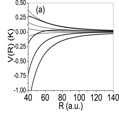
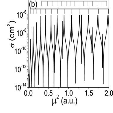
Figure 1: (a) Adiabatic curves of the pure dipole system for two values of the dipole moment $\mu$: $\mu=0.1$ (gray) and $\mu=1$ (black) (b) The cross section of the polarized dipole model versus $\mu$, at a collision energy $E=10^{-12}$ K. The brackets denote predicted resonant positions using the adiabatic WKB phase (AWP) approximation. The black bracket represents for the phase contribution from the lowest adiabatic curve and the gray is from all remaining contributions.

Our primary interest in polar molecule scattering is how the strong anisotropic interaction affects the system. As a first step illustrating the influence of dipolar interactions, we present a simple model composed of polarized dipoles with no internal structure. Strictly speaking, this system is created by an infinitely strong electric field that completely polarizes the molecules and raises all other internal states to experimentally unattainable energies. Thus the only label required for a channel is its partial wave, $l=\{0,2,4,...\}$ in the numerical example given here. The matrix elements of the dipole-dipole interaction are taken to be $\langle 12l0|H_{\mu\mu}|12l^{\prime}0\rangle=-0.32\mu^{2}\langle l0|C_{0}^{2}|l^{\prime}0\rangle$, which is typical for molecules like RbCs or SrO. We then artificially vary the dipole moment $\mu$ to see the effect of an increasingly strong dipolar interaction. Pragmatically speaking, varying $\mu$ parallels changing the electric field. The intention of this model is to focus on the effect of direct anisotropic couplings between the degenerate channels, as measured by their effect on the partial wave channels.

For this model, we use a reduced mass of $m_{r}=10^{4}$ a.u., typical of very light molecules. We moreover assume that the molecules approach one another along the laboratory z-axis, so that only the projection $m_{l}=0$ of orbital angular momentum is relevant. To set a concrete boundary condition at small $R$, we apply “hard wall” boundary conditions, $\psi(R_{in})=0$ at a characteristic radius $R_{in}=20$ a.u. (In Sec. V we will relax this restriction.) We pick the collision energy to be nearly zero, namely $10^{-12}$ K. To converge the calculation for this model requires inclusion of partial waves up to $l=14$, and numerical integration of the Schrödinger equation out to $R=R_{\infty}=1\times 10^{5}$ a.u., using the log-derivative propagator method of Johnson Johnson .

To get a sense of the influence of increasing the dipole moment, we first look at adiabatic curves of the system. Figure 1 (a) shows two different sets of adiabatic curves: a gray set with $\mu=0.1$ (a.u.) and a black set $\mu=1.0$ (a.u.). In each set, the four lowest adiabatic curves are shown. Looking at these curves, we can see two characteristic effects of increasing $\mu$. First, the lowest curve becomes much deeper. Second, the higher adiabatic curves, originating form non-zero partial waves, may support bound states at short distance states, i.e. within the centrifugal barrier. Both these effect may generate bound states, leading to distinct classes of scattering resonances as $\mu$ is varied. The deepening of the lowest adiabatic curves induces potential resonances, whereas the higher-lying curves lead to narrow shape resonances, wherein the molecules must tunnel through the centrifugal barrier.

The different classes of resonances can clearly be seen in cross section, as shown in Fig. 1 (b). The broad quasi-regular set of resonances seen in the cross section are the potential resonances originating from the lowest adiabatic curve. The narrow shape resonances appearing sporadically in the spectrum originate from the higher-lying curves. For the purpose of this paper, we focus on the wide potential resonances and simply acknowledge the existence of the narrow shape resonances.

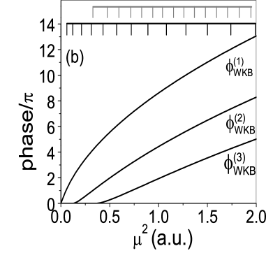
Figure 2: (a) Eigenphase (solid) and total adiabatic WKB phase (AWP,dashed) for the dipole-scattering model. (b) AWP contributions for the lowest adiabatic curves ($\phi^{(1)}_{WKB}$) with the black bracket indicating when $\phi^{(1)}_{WKB}$ passes through a multiple of $\pi$. The two remaining curves are contributions with non-zero partial waves ($\phi^{(2,3)}_{WKB}$). The gray bracket indicates where the sum of these contributions pass through a multiple of $\pi$.

To show that the broad resonances primarily belong to the lowest potential and the narrow shape resonances belong to the higher-lying potentials, we use an eigenphase analysis. The eigenphase can be thought of as the sum of the phase shifts for all of the channels; thus it tracks the behavior of all the channels simultaneously. The eigenphase is defined as

$$\phi_{eigen}=\sum_{i}\tan^{-1}(\lambda_{i}^{K}).$$ (32)

Here $\lambda_{i}^{K}$ are the eigenvalues of the $K$ matrix from the full-scattering calculation Taylor . (The $K$ matrix is related to the more familiar scattering matrix by $S=(1+iK)/(1-iK)$.) When the system gains a bound state, it appears as a $\pi$ jump in eigenphase. The eigenphase of the system is shown in Fig. 2 (a), as the solid line with many abrupt steps.

To analyze this situation further, we construct an approximate eigenphase as follows. First, we asses the total phase accumulated in each adiabatic channel, using a WKB prescription:

$$\phi_{WKB}^{(i)}(\mu)=\int_{R_{in}}^{R_{out}}\sqrt{-2m_{r}V_{AD}^{(i)}(\mu,R)/\hbar^{2}}.$$

Here $(i)$ stands for the $i^{th}$ adiabatic curve. For the lowest adiabatic curve, which is always attractive, the range of integration is from $R_{in}$ to $R_{out}=\infty$. For high-lying channels that possess a barrier to scattering at zero collision energy, the limits of integration are from $R_{in}$ to the inner classical turning point of the barrier. This will yield some information on shape resonances trapped behind the barrier, but we will not make much of this in the analysis to follow. Finally, we add together the individual WKB phases to produce an approximate eigenphase shift, which we dub the “adiabatic WKB phase” (AWP):

$$\phi_{WKB}(\mu)=\sum_{i}\phi_{WKB}^{(i)}(\mu),$$ (33)

Since we are not concerned with properties of the phase associated with the higher-lying adiabatic curves, we do not consider the connection formula now.

The total AWP for this system is shown as a dashed line in Fig. 2 (a). It tracks the eigenphase well but offers more information if we decompose the AWP into its contributions. Figure 2 (b) shows the individual contributions of the sum. The largest contribution is the phase from the lowest adiabatic curve, which can be associated with potential resonances. A black bracket appears above this phase contribution with vertical marks indicating when it passes through an integer multiple of $\pi$, i.e., when we expect to see a potential resonance in the cross section. This same bracket is plotted in Fig. 1 and shows good agreement between the locations of the potential resonances and the AWP predictions. We conclude from this that the main resonance features in the Stark spectrum arise primarily from this single potential curve.

In Fig. 2 (b) the two remaining phase contributions originate from non-zero partial wave channels that possess centrifugal barriers; see Fig. 1(b). The gray bracket indicates where the sum of these two contributions pass through an integer multiple of $\pi$, and thus represent a guess for where the shape resonances lie. This gray bracket is also shown in Fig. 1. The agreement with the position of the narrow resonance features in the cross section is not nearly as good as it is with the broad potential resonances. This indicates a more involved criterion for shape resonances. Nevertheless, the AWP predicts 15 shape resonances, and there are 13 in the range of $\mu$ shown. The AWP appears to offer a means to roughly predict the number of shape resonances in this system, even though it does not predict the locations exactly.

A main point of this analysis is that the AWP in the lowest adiabatic channel alone is sufficient to locate the potential (as opposed to shape) resonances, without further modification. For the rest of this paper, we focus on the potential resonances in more realistic molecules with internal molecular structure. The general analysis in terms of a single-channel AWP will still hold, but an additional phase shift will be required to describe the spectrum.

IV Strong Field Seekers

Strong-field-seeking molecules are approximately described as polarized in the sense of the last section, because their dipole moments are aligned with the field. They will, however, contain a richer resonance structure owing to the presence of low-lying excited states that can alter the dipolar potential energy surface at small-$R$.

For concreteness, we focus here on molecules with a ${}^{1}\Sigma$ ground state. Heteronulcear alkalis fit into this category and are rapidly approaching ground state production with various species alkali . As examples, we pick RbCs and SrO in their ground states. Ground state RbCs has been produced experimentally Sage . As for SrO, promising new techniques should lead to experimental results soon Demille . For simplicity we include only the $J=0$, $J=1$ rotational states, and freeze the projection of molecular angular momentum to $M_{J}=0$. This restricts the number of scattering thresholds to three, identified by the parity quantum number of the molecules in zero field. The parity quantum numbers for the three thresholds are ($--,-+,++$). This model is similar to the one presented in Ref. AA_PRA which can be easily constructed for any rigid rotor when only including two molecular states. One immediate consequence of multiple thresholds is the presence of rotational Fano-Feshbach resonances in the collisional spectrum.

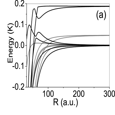
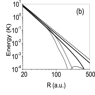
Figure 3: (a) Adiabatic curves for the RbCs system at two different field values, ${\cal E}=0(V/cm)$ (gray) and ${\cal E}=5000(V/cm)$ (black). (b) Log-log plot of the absolute value of the two lowest adiabatic curves The blue dashed line is proportional to $1/R^{3}$.

The first example is RbCs, whose physical parameters are $\mu=1.3$ D, $m_{r}=110$ a.m.u., and $B_{e}=0.0245(K)$ Sage . As before, we apply vanishing boundary condition at $R_{in}=20$ a.u. To converge this calculation over the field range considered, we require partial waves up to $l=30$. We first look at the adiabatic curves of the system to get an understanding of how the real system deviates from the simple model presented above. In Fig. 3 (a) we plot the 6 lowest adiabatic curves for the RbCs system with only four partial waves, so the figure is more easily interpreted. The sets of adiabatic curves shown are for two different field values: the gray set has $\cal E$=0 and the black set has $\cal E$= 5000 (V/cm). There are two important features that differ from the dipole example. First, there are two higher thresholds, and the electric field shifts these apart in energy as the field is increased. Second,the electric field dramatically changes the radial dependence of the Hamiltonian.

The difference in thresholds can be seen clearly in Fig. 3 (a) where the lowest excited threshold moves from $0.05(K)$ at $\cal E$=0 to $0.18(K)$ at $\cal E$=5000 (V/cm). The difference in radial dependences for the two cases is seen more clearly in a log-log plot of the two lowest adiabatic curves for both fields, as shown in Fig. 3 (b). The gray set corresponding to zero field has two distinct asymptotic radial powers. At large $R$ the lowest adiabatic curve has a $1/R^{6}$ behavior asymptotically because of couplings with channels far away in energy [$\sim 0.05(K)$]. However as $R$ approaches zero the dipolar interaction has overwhelmed the rotational energy separation and the radial dependence becomes $1/R^{3}$ in character at about R=100 (a.u.). For reference, the dashed line is proportional to $1/R^{3}$. With $\cal E$= 5000 (V/cm), the two black curves show the radial dependence of the adiabatic curves. The lowest curve now has nearly $1/R^{3}$ over the whole range shown. Asymptotically when the centrifugal barrier is larger, the radial dependence will change to $1/R^{4}$ AA_PRA . The second lowest adiabatic curve is also significantly altered by the strong dipolar interaction as can be seen in Fig. 3 (b).

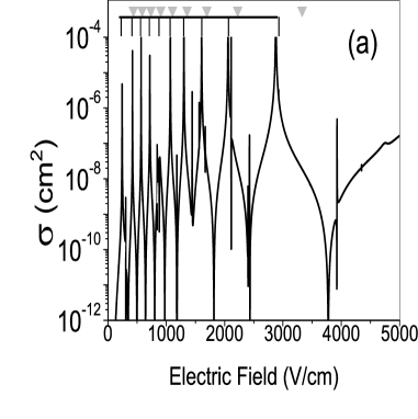
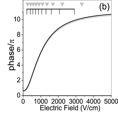
Figure 4: (a) Cross section for RbCs in strong-field seeking states, including the 10 potential resonances that the AWP predicts (solid bracket). The AWP phases are shown in (b). The black bracket corresponds to the AWP predicted resonances for the lowest adiabatic curve after a defect, $\delta_{defect}=0.14$, has been added according to Eq. (34). The gray triangles are the AWP predicted resonances without the defect.

In Fig. 4 (a), we plot the cross section for the model RbCs system. This spectrum is riddled with narrow Fano-Feshbach resonances, but is still dominated by a series of potential resonances similar to the one in Fig. 1 (b). There are two sets of AWP predictions shown as over-brackets. To understand their difference, we look to Fig. 4 (b). The AWP for the lowest adiabatic curve is shown in Fig. 4 (b) for two different zero-field phase values. The gray curve is the AWP that is directly computed from the method described above, Eq. (33). The locations where it passes through an integer multiple of $\pi$ are indicated by the gray triangles. Referring back to Fig. 4 (a), where the same gray triangles appear we see that this simple estimate does not reproduce the resonance position.

We can, however, introduce an additional overall phase shift to account for the difference in short-range interactions from the pure polarized case. The shifted AWP reads

$$\tilde{\phi}_{WKB}^{(1)}({\cal E})=\phi_{WKB}^{(1)}({\cal E})+\pi\delta_{defect}.$$ (34)

By treating $\delta_{defect}$ as a fitting parameter, we can obtain the resonance positions indicated by the black bracket in Fig. 4, which agree quite well with the resonance positions in the close-coupled calculation. To do so requires, in this case, a phase shift $\delta_{defect}=0.14$. In analogy with Rydberg spectroscopy we consider the shift we have added to be a “quantum defect” that accounts for the effect of the short-range interaction. The additional phase shift reflects the influence of short range physics on the scattering, such as curve crossings with curves from higher thresholds.

The AWP also saturates with field, as can be seen in Fig. 4 (b). This occurs because the electric field eventually fully polarizes the molecules, so the dipole moment cannot increase further. The effect can also be seen in the spacing of the potential resonances. At low fields, the potential resonances occur frequently in field. Then, as the field is further increased, the resonances occur less often in field, which is a signature of dipole moment saturating and therefore an increasing field having less effect on the molecular interaction.

Figure 5: Cross section for SrO with a bracket indicating resonance positions predicted by the phase shifted AWP for the lowest adiabatic curve. There are 33 PR shown in this range of electric field. $\delta_{defect}=0.215$

As a second example, we consider SrO, which has the physical parameters $m_{r}$=52 a.m.u, $\mu$=8.9 D, and $B_{e}=$ 0.5 K Demille . We choose this molecule for its comparatively large mass and dipole moment, which guarantee a large number of resonances. Fig. 5 we have plotted the cross section for SrO, which is dominated by the quasi-regular potential resonance series. As before, the black bracket indicates where the phase shifted AWP predicts the potential resonances, and we see the agreement is good. Furthermore, the series has not terminated since we have not completely polarized the dipole. The series of potential resonances saturates at 17.5 (kV/cm) after a total of 43 potential resonances have been induced. To line up the AWP’s predictions and the actual cross section requires a defect of $\delta_{defect}=0.215$.

We have picked two examples to illustrate how the potential resonances will appear in the context of collisional spectroscopy. These resonance will occur to varying degrees in the strong-field seeking collisions of all polar molecules. For example, we can also make similar predictions for an asymmetric rotor molecule such as formaldehyde $(H_{2}CO)$. We find that this molecule should possess six potential resonances in the field interval from 0 to 50 $(kV/cm)$.

It is worth noting that portions of similar resonance series was anticipated in cold atomic gases subjected to electric fields Deb . However very few such resonances are likely to be observed, owning to the enormous fields ($\sim MV/cm$) required to generate them. In polar molecules, by contrast, the entire series should be readily observable.

V Collisional Spectroscopy

Through the course of this work we have shown that the zero-energy cross section of weak-field-seeking molecules is dominated by a set of broad potential resonances. Even though these resonances are themselves intriguing, their properties can be exploited to learn much more about the system. The general structure of the potential resonances is governed by the long range dipolar interaction, which has a predictable and common form. With a clear understanding of this interaction and how it induces resonances, it could be exploited to learn about the short range interaction of the molecules. This is because details of where the lines appear must also depend on the boundary condition experienced by the wave function at small values of $R$. Therefore the spectrum contains information on the small $R$ intermolecular dynamics. Thus by studying the potential resonance series we can extract information about the short range dynamics.

This idea is similar to quantum defect theory, which, for example, has been very successful in Rydberg spectroscopy. The short range physics of the electron interacting with the nucleus is complicated and not easily solved. However once the electron is out of the small $R$ region, it enters into a pure coulomb potential where the motion of the electron is well understood. The effect of the short range must be merged with the long range physics to form a complete solution. To account for the short range interaction, the energy can be parameterized by replacing the principal quantum number by an effective quantum number $n^{\star}=n-\mu$. This procedure is tantamount to identifying an additional phase shift due to the interaction of the electron with the atomic core. The idea of merging standard long range physics with complicated short range behavior has been applied successfully not only in Rydberg states of atoms qdt ; Fano and molecules Jungen , but also in atomic collisions Mies , cold collisions Greene2 ; Mies2 ; Gao , and dipole-dipole interactions of the type we envision here Deb .

Figure 6: The vertical curves represent electric field values where the AWP predicts potential resonances for a given defect, ${\cal E}_{WKB}(\delta_{defect})$. The points represent resonant field values, ${\cal E}^{(b)}$, in the full calculations with different initial boundary conditions. The values of $b$ are given by cotan$(\pi\beta)$ and $\beta$ for the different full numerical calculations are $0$ (filled circle), $0.11$ (filled square), $0.22$ (filled triangle), $0.56$ (hollow circle), $0.78$ (hollow square), and $0.89$ (hollow triangle). Each set of values ${\cal E}^{(b)}$ is plotted at a height corresponding to its best-fit value of $\delta_{defect}$.

As a simple expression of this idea, we can alter the boundary condition applied at $R_{in}$ when performing the full scattering calculation and note its influence on the field dependent spectrum. For the above calculations we have imposed the standard vanishing boundary condition, $\psi(R_{in})=0$ for all channels. We now replace this condition with a uniform logarithmic derivative, $b=({d\over dR}\psi)\psi^{-1}$, at $R_{in}$. Thus previously we set $b=\infty$, but now we allow $b$ to vary. The log-derivative is conveniently represented as a phase:

$$b={\rm cotan}(\pi\beta),$$ (35)

where $\beta$ can lie between zero and one, covering all values of $b$ from $-\infty$ to $+\infty$. For $\beta=0$, the boundary condition is the one employed above, $\psi(R_{in})=0$, whereas for $\beta=0.5$, the boundary condition is ${d\over dR}\psi(R_{in})=0$.

We have re-computed the collisional spectrum of RbCs for several different initial conditions, and plotted the field values of the potential resonances, ${\cal E}^{(b)}$, in Fig. 6 as sets of points. The values of $\beta$ for the different calculations are $0$ (filled circle), $0.11$ (filled square), $0.22$ (filled triangle), $0.56$ (hollow circle), $0.78$ (hollow square), and $0.89$ (hollow triangle). The filled circles are resonant locations for cross section in Fig. 4 (a).

We next wish to demonstrate that each such spectrum can be identified by a single quantum defect parameter, as was done in the previous section. This entails picking a value of $\delta_{defect}$ and then setting the phase $\tilde{\phi}_{WKB}^{(1)}({\cal E})$ equal to an integer multiple of $\pi$. This yields a set of resonant field values, ${\cal E}_{WKB}(\delta_{defect})$. Each $\delta_{defect}$ corresponds to a particular approximate spectrum. The set of curves, ${\cal E}_{WKB}(\delta_{defect})$, generated by continuously varying $\delta_{defect}$ are shown are shown in Fig. 6 as solid lines. The bracket in Fig. 4 (a) corresponds to the set of points where a vertical line intersects ${\cal E}_{WKB}(\delta_{defect})$ with $\delta_{defect}=0.14$.

We can compare the the resonant field values predicted by the AWP, ${\cal E}_{WKB}(\delta_{defect})$, and resonant field values given by the full calculation with different initial conditions, ${\cal E}^{(b)}$. To plot ${\cal E}^{(b)}$ we have varied the height at which the set of points ${\cal E}^{(b)}$ is plotted until it aligns with ${\cal E}_{WKB}(\delta_{defect})$. Doing this we are able to to see how $b$ and $\delta_{defect}$ are related. Thus in fig. 6 we can see that even with different boundary conditions, the single AWP curve in fig 4 (b) can be used to predict the spacing between the potential resonances by varying a single parameter, $\delta_{defect}$. This shows the AWP represents the long range scattering physics well, and that empirically extracted parameters like $\delta_{defect}$ will carry information about the short-range physics such as that embodied in $b$.

VI Conclusion

A number of resonant processes may occur when two polar molecules meet in an ultracold gas. We have focused here on the dominant, quasi-regular, series of potential resonances between weak-field seeking states. These potential resonances originate in the direct deformation of the potential energy surface upon which the molecules scatter. Observation of these resonances may offer a direct means for probing the short range interaction between molecules. We have provided a means of analyzing this system with an adiabatic WKB phase integral. This method shows how the system evolves with the application of an electric field.

- (1) N. R. Claussen, et al., Phys. Rev. A 67, 060701 (2003); E. G. M. van Kempen, et al., Phys. Rev. Lett. 88, 093201 (2002); K. M. O’Hara et al. Phys. Rev. A 66, 041401(R) (2002); C. Chin, et al. Phys. Rev. Lett. 85, 2717 (2000); J. P. Leo, et al. Phys. Rev. Lett. 85, 2721 (2000).
- (2) J. Doyle, B. Friedrich, R.V. Krems, and F. Masnou-Seeuws, Eur. Phys. J. D 31, 149 (2004).
- (3) J. L. Bohn, A. V. Avdeenkov, and M. P. Deskevich Phys. Rev. Lett. 89, 203202 (2002).
- (4) P. Florian, M. Hoster, and R. C. Forrey, Phys. Rev. A 70, 032709 (2004).
- (5) N. Balakrishnan, R. C. Forrey, and A. Dalgarno, Phys. Rev. Lett. 80, 3224 (1998).
- (6) R. V. Krems, Phys Rev. Lett. 93 13201 (2004).
- (7) M. Marinescu and L. You, Phys Rev. Lett. 81 4596 (1998); S. Yi and L. You, Phys. Rev. A 63, 053607 (2001).
- (8) B. Deb and L. You, Phys. Rev. A 64, 022717 (2001).
- (9) A.V. Avdeenkov and J. L. Bohn, Phys. Rev. Lett. 90, 043006 (2003).
- (10) A.V. Avdeenkov and J. L. Bohn, Phys. Rev. A 66, 052718 (2002).
- (11) A. V. Avdeenkov, D. C. E. Bortolotti, and J. L. Bohn, Phys. Rev. A 69 12710 (2004).
- (12) A. Derevianko, S. G. Porsev, S. Kotochigova, E. Tiesinga, and P. S. Julienne, Phys. Rev. Lett. 90, 063002 (2003)
- (13) R. Santra et. al, Phys. Rev. A 67, 062713 (2003).
- (14) G. D. Stevens, et al., Phys Rev. A 53 1349 (1996).
- (15) J. F. Baugh, et al., Phys Rev. A 58 1585 (1998).
- (16) M. J. Seaton, Rep. Prog. Phys. 46 167 (1983).
- (17) M. Aymar et al., Rev Mod. Phys. 68, 1015 (1996).
- (18) C. Ticknor and J. L. Bohn, Phys. Rev. A 71 22706 (2005).
- (19) C. Ticknor, PhD. Thesis, University of Colorado (unpublished), 2005.
- (20) J. Brown and A. Carrington, Rotational Spectroscopy of Diatomic Molecules, (Cambridge, Cambridge, 2003).
- (21) D. M. Brink and G. R. Satchler, Angular Momentum, (Clardeon Press, Oxford, 1993).
- (22) K. Schreel and J. J. ter Muelen, J. Phys. Chem. A 101, (1997).
- (23) T. Hain, R. Moision, and T. Curtiss, J. Chem. Phys. 111, 6797 (1999).
- (24) M. Tinkham, Group Theory and Quantum Mechanics, (Dover, New York, 2003).
- (25) B. R. Johnson, J. Comput. Phys. 13, 445 (1973).
- (26) J. R. Taylor, Scattering Theory (Krieger, Florida, 1983).
- (27) C. Haimberger et al., Phys. Rev. A 70, 021402 (R) (2004); A. J. Kerman, et. al Phys. Rev. Lett. 92, 153001 (2004); D. Wang et al., Phys. Rev. Lett. 93, 243005 (2004); M. W. Mancini, et al., Phys. Rev. Lett. 92, 133203 (2004).
- (28) J. Sage, et al., Phys. Rev. Lett 94 203001 (2005).
- (29) D. DeMille, D.R. Glenn, and J. Petricka, Eur. Phys. J. D 31, 375-384 (2004).
- (30) U. Fano and A. R. P. Rau, Atomic Collisions and Spectra (Academic Press, London, 1986).
- (31) C. H. Greene and Ch. Jungen, Adv. At. Mol. Phys. 21, 51 (1985).
- (32) F. H. Mies, J. Chem. Phys. 80, 2514 (1984).
- (33) B. Gao, Phys. Rev. A 58, 4222 (1998); ibid. 62, 050702 (2000).
- (34) J. P. Burke, Jr., C. H. Greene, and J. L. Bohn, Phys. Rev. Lett. 81, 3355 (1998).
- (35) F. H. Meis and M. Raoult, Phys. Rev. A 62, 012708 (2000).