Transmission matrix of a uniaxial optically active crystal platelet

Abstract

Expressions corresponding to the transmission of a uniaxial optically active crystal platelet are provided for an optical axis parallel and perpendicular to the plane of interface. The optical activity is taken into account by a consistent multipolar expansion of the crystal medium response due to the path of an electromagnetic wave. Numerical examples of the effect of the optical activity are given for quartz platelets of chosen thicknesses. The optical activity’s effects on the variations of the transmission of quartz platelets as a function of the angle of incidence is also investigated.

LAL 05-21
May 2005

1 Introduction

Optical activity in crystals is a phenomenon which has been known for a long time (see Ref. [1] for an historical review). Two methods are currently used to describe the effect of the crystal optical activity on plane wave propagation. The first one is phenomenological and is valid under normal incidence [2, 3, 4, 5, 6, 7]. The second one is a first principle method and consists in solving the Maxwell equations with modified constitutive equations [1, 8, 9, 10] (i.e. the relationship between the electric and magnetic fields vectors and the electric displacement and magnetic induction field vectors). The choice of the constitutive equations is of prior importance [9] and was itself of phenomenological nature until the link between the optical activity as well as the magnetic-dipole and electric-octupole responses of the crystal medium was consistently formalised[11, 12]. This theory leads to constitutive equations different from those previously used. To the author’s knowledge, the constitutive equations of Ref. [11] have not yet been used to calculate the transmission matrix of an optical active uniaxial platelet. They were only applied to describe the reflection of a plane wave by an interface between an isotropic achiral and a uniaxial chiral media [13], but for an optical axis parallel or perpendicular to the plane of incidence. It is the purpose of this article to provide this transmission matrix in a simple and usable form. We further restrict ourselves to two geometric configurations often encountered experimentally, namely the optical axis parallel and perpendicular to the plane of interface.

Recent experimental results have shown that the contribution of the optical activity to the transmission matrix of a quarter wave plate can reach the percent level [6]. As an application of our transmission matrix formula, the origin of this effect is investigated and the case of half wave plates is also considered. Our formula being valid under oblique incidence, numerical calculations of the variations of the platelet transmission matrix as a function of the angle of incidence are presented.

In section 2 we describe the method. In section 3, we derive the explicit expressions of the platelet transmission matrix for oblique and normal incidences. The contribution of the optical activity to the transmission matrix is studied numerically for various quartz platelet thicknesses in section 4.

2 Formalism

A monochromatic plane wave of wavelength $\lambda$ impinging a uniaxial optically active crystal slab of thickness $\ell$ is considered. The crystal is assumed to be non-absorbing, non-magnetic and surrounded by an isotropic achiral ambient medium.

A direct axis system $x,y,z$ is defined such that the $z$ axis is perpendicular to the plane of interface. The origin of the $z$ axis (i.e. $z=0$) is fixed on the first plane of interface so that $z=\ell$ corresponds to the second plane of interface (see Fig. 1). The unit vector basis attached to the system axes is denoted $\{\mbox{${\rm\bf\hat{x}}$},\mbox{${\rm\bf\hat{y}}$},\mbox{${\rm\bf\hat{z}}$}\}$.Without loss of generality, the plane of incidence is taken to be $yz$. To determine the transmission and reflection matrices of the interfaces between the ambient medium and the crystal faces, we follow the method of Ref. [14].

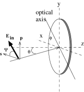
Figure 1: Schematic view of an optically active platelet with its optical axis in the plane of interface. The angles and axes used in the calculations are also drawn.

Near the first interface $z=0$, the electric and magnetic field vectors read:

$$\hbox{Incident: }\mbox{${\rm\bf E}$}= \biggl{[}A_{s}\mbox{${\rm\bf\hat{s}}$}+A_{p}\mbox{${\rm\bf\hat{p}}$}\biggr{]}\exp(i[\omega t-\mbox{${\rm\bf k}$}\cdot\mbox{ ${\rm\bf r}$}])$$ (1)

$$\mbox{${\rm\bf H}$}= \frac{1}{\mu_{0}\omega}\mbox{${\rm\bf k}$}\times\biggl{[}A_{s}\mbox{${\rm\bf\hat{s}}$}+A_{p}\mbox{${\rm\bf\hat{p}}$}\biggr{]}\exp(i[\omega t-\mbox{${\rm\bf k}$}\cdot\mbox{ ${\rm\bf r}$}])$$ (2)

$$\hbox{ Reflected: }\mbox{${\rm\bf E}$}= \biggl{[}B_{s}\mbox{${\rm\bf\hat{s}}$}+B_{p}\mbox{${\rm\bf\hat{p}}$}^{\prime}\biggr{]}\exp(i[\omega t-\mbox{${\rm\bf k}$}^{\prime}\cdot\mbox{ ${\rm\bf r}$}])$$ (3)

$$\mbox{${\rm\bf H}$}= \frac{1}{\mu_{0}\omega}\mbox{${\rm\bf k}$}^{\prime}\times\biggl{[}B_{s}\mbox{${\rm\bf\hat{s}}$}+B_{p}\mbox{${\rm\bf\hat{p}}$}^{\prime}\biggr{]}\exp(i[\omega t-\mbox{${\rm\bf k}$}^{\prime}\cdot\mbox{ ${\rm\bf r}$}])$$ (4)

$$\hbox{Refracted: }\mbox{${\rm\bf E}$}= \biggl{[}C_{o}\mbox{${\bf o}$}_{+}\exp(-i\mbox{$\rm\bf k_{o}$}_{+}\cdot\mbox{ ${\rm\bf r}$})+C_{e}\mbox{${\bf e}$}_{+}\exp(-i\mbox{$\rm\bf k_{e}$}_{+}\cdot\mbox{ ${\rm\bf r}$})\biggr{]}\exp(i\omega t)$$ (5)

$$\mbox{${\rm\bf H}$}= \frac{1}{\mu_{0}\omega}\biggl{[}C_{o}(\mbox{$\rm\bf k_{o}$}_{+}\times\mbox{${\bf o}$}_{+}-i\mu_{0}\omega{\mathcal{T}}\mbox{${\bf o}$}_{+})\exp(-i\mbox{$\rm\bf k_{o}$}_{+}\cdot\mbox{ ${\rm\bf r}$})+$$

$$C_{e}(\mbox{$\rm\bf k_{e}$}_{+}\times\mbox{${\bf e}$}_{+}-i\mu_{0}\omega{\mathcal{T}}\mbox{${\bf e}$}_{+})\exp(-i\mbox{$\rm\bf k_{e}$}_{+}\cdot\mbox{ ${\rm\bf r}$})\biggr{]}\exp(i\omega t)$$ (6)

and near the second interface $z=\ell$:

$$\hbox{Reflected: }\mbox{${\rm\bf E}$}= \biggl{[}C^{\prime}_{o}\mbox{${\bf o}$}_{-}\exp(-i\mbox{$\rm\bf k_{o}$}_{-}\cdot\mbox{ ${\rm\bf r}$})+C^{\prime}_{e}\mbox{${\bf e}$}_{-}\exp(-i\mbox{$\rm\bf k_{e}$}_{-}\cdot\mbox{ ${\rm\bf r}$})\biggr{]}\exp(i\omega t)$$ (7)

$$\mbox{${\rm\bf H}$}= \frac{1}{\mu_{0}\omega}\biggl{[}C^{\prime}_{o}(\mbox{$\rm\bf k_{o}$}_{-}\times\mbox{${\bf o}$}_{-}-i\mu_{0}\omega{\mathcal{T}}\mbox{${\bf o}$}_{-})\exp(-i\mbox{$\rm\bf k_{o}$}_{-}\cdot\mbox{ ${\rm\bf r}$})+$$

$$C^{\prime}_{e}(\mbox{$\rm\bf k_{e}$}_{-}\times\mbox{${\bf e}$}_{-}-i\mu_{0}\omega{\mathcal{T}}\mbox{${\bf e}$}_{-})\exp(-i\mbox{$\rm\bf k_{e}$}_{-}\cdot\mbox{ ${\rm\bf r}$})\biggr{]}\exp(i\omega t)$$ (8)

$$\hbox{Refracted: }\mbox{${\rm\bf E}$}= \biggl{[}A^{\prime}_{s}\mbox{${\rm\bf\hat{s}}$}+A^{\prime}_{p}\mbox{${\rm\bf\hat{p}}$}\biggr{]}\exp(i[\omega t-\mbox{${\rm\bf k}$}\cdot\mbox{ ${\rm\bf r}$}])$$ (9)

$$\mbox{${\rm\bf H}$}= \frac{1}{\mu_{0}\omega}\mbox{${\rm\bf k}$}\times\biggl{[}A^{\prime}_{s}\mbox{${\rm\bf\hat{s}}$}+A^{\prime}_{p}\mbox{${\rm\bf\hat{p}}$}\biggr{]}\exp(i[\omega t-\mbox{${\rm\bf k}$}\cdot\mbox{ ${\rm\bf r}$}])$$ (10)

with the incident field vectors given by Eqs. (5,6).

In these expressions, ${\rm\bf k}$ and $\mbox{${\rm\bf k}$}^{\prime}$ are the wave vectors in the ambient medium; the three vectors ${\rm\bf\hat{s}}$, ${\rm\bf\hat{p}}$ and ${\rm\bf k}$ form a direct basis, they are given by $\mbox{${\rm\bf\hat{s}}$}=\mbox{${\rm\bf\hat{p}}$}\times\mbox{${\rm\bf k}$}/|\mbox{${\rm\bf\hat{p}}$}\times\mbox{${\rm\bf k}$}|$ and $\mbox{${\rm\bf\hat{s}}$}=\mbox{${\rm\bf\hat{p}}$}^{\prime}\times\mbox{${\rm\bf k}$}^{\prime}/|\mbox{${\rm\bf\hat{p}}$}^{\prime}\times\mbox{${\rm\bf k}$}^{\prime}|$ with ${\rm\bf\hat{s}}$ perpendicular to the plane of incidence (i.e. $\mbox{${\rm\bf\hat{s}}$}=\mbox{${\rm\bf\hat{x}}$}$); ${\mathcal{T}}$ is a second-rank tensor coming from the constitutive equations [11], its components are related to those of the gyration tensor coefficients $g_{ij}$ [2]; the electric vectors $\mbox{${\bf o}$}_{\pm}$ and $\mbox{${\bf e}$}_{\pm}$ are the solutions of the wave equation inside the crystal; the wave vectors inside the medium, $\mbox{$\rm\bf k_{o}$}_{\pm}$ and $\mbox{$\rm\bf k_{e}$}_{\pm}$, are given by the Snell’s law and by the condition of existence of solutions of the wave equation.

The wave equation inside the crystal is given by [11]

$$\sum_{\beta}\biggl{(}k_{\alpha}k_{\beta}-\delta_{\alpha\beta}k^{2}+\mu_{0}\omega^{2}\epsilon_{\alpha\beta}+i\mu_{0}\omega\sum_{\gamma}k_{\gamma}{\mathcal{A}}_{\alpha\beta\gamma}\biggr{)}E_{\beta}=0$$ (11)

where $\alpha,\beta$ and $\gamma$ stand for $x$ or $y$ or $z$ and where the magnetic-dipole and electric-quadrupole response of the medium is embodied in the third-rank tensor ${\mathcal{A}}$ whose components are related to those of the gyration tensor[11, 13]. In Eq. (11), $k_{\alpha}$ stands for the components of one of the four wave vectors $\mbox{$\rm\bf k_{o}$}_{\pm}$ and $\mbox{$\rm\bf k_{e}$}_{\pm}$; $E_{\beta}$ stands for one of the components of the four electric vectors $\mbox{${\bf o}$}_{\pm}$ and $\mbox{${\bf e}$}_{\pm}$; $\epsilon_{\alpha\beta}$ are the elements of the dielectric tensor.

The wave amplitudes are related by matrix relations. The refraction by the first (i.e. $z=0$) and second (i.e. $z=\ell$) interfaces are described by [14]:

$$\begin{pmatrix}C_{o}\\ C_{e}\end{pmatrix}=T\begin{pmatrix}A_{s}\\ A_{p}\end{pmatrix}\,\hbox{ and }\begin{pmatrix}A^{\prime}_{s}\\ A^{\prime}_{p}\end{pmatrix}=T^{\prime}P_{+}\begin{pmatrix}C_{o}\\ C_{e}\end{pmatrix}$$ (12)

respectively. As for the reflections by the first and second crystal-ambient medium interfaces (inside the crystal), one gets

$$\begin{pmatrix}C_{o}\\ C_{e}\end{pmatrix}=R\begin{pmatrix}C^{\prime}_{o}\\ C^{\prime}_{e}\end{pmatrix}\,\hbox{ and }\begin{pmatrix}C^{\prime}_{o}\\ C^{\prime}_{e}\end{pmatrix}=P_{-}^{-1}RP_{+}\begin{pmatrix}C_{o}\\ C_{e}\end{pmatrix}$$ (13)

respectively. In the previous equations, the following $2\times 2$ phase matrices were introduced:

$$P_{\pm}=\begin{pmatrix}\exp(-i\varphi_{o_{\pm}})&0\\ 0&\exp(-i\varphi_{e_{\pm}})\\ \end{pmatrix},\,$$ (14)

with $\varphi_{o_{\pm}}=\ell(\mbox{$\rm\bf k_{o}$}_{\pm}\cdot\mbox{${\rm\bf\hat{z}}$})$ and $\varphi_{e_{\pm}}=\ell(\mbox{$\rm\bf k_{e}$}_{\pm}\cdot\mbox{${\rm\bf\hat{z}}$})$.

The $2\times 2$ matrices $T$, $T^{\prime}$ and $R$ are obtained from the continuity conditions of the projections of the electric and magnetic field vectors in the planes $z=0$ and $z=\ell$. Once known, these matrices are used to compute the platelet transmission matrix $M$ such that $\mbox{${\rm\bf E_{out}}$}=M\mbox{${\rm\bf E_{in}}$}$ where ${\rm\bf E_{in}}$ and ${\rm\bf E_{out}}$ are the electric field vectors before and after the crystal slab respectively. Note that $M$, ${\rm\bf E_{in}}$ and ${\rm\bf E_{out}}$ are thus represented in the $\{\mbox{${\rm\bf\hat{s}}$},\mbox{${\rm\bf\hat{p}}$},\mbox{${\rm\bf\hat{k}}$}\}$ basis, so that $M$ reduces to a $2\times 2$ matrix and ${\rm\bf E_{in}}$ and ${\rm\bf E_{out}}$ to two-dimension vectors when plane waves are considered.

Taking into account the multiple reflections inside the crystal, one gets:

$$M=T^{\prime}P_{+}T+T^{\prime}P_{+}RP_{-}^{-1}RP_{+}T+\cdots=T^{\prime}P_{+}\biggl{[}{\underline{1}}-RP_{-}^{-1}RP_{+}\biggr{]}^{-1}T$$ (15)

where we have used $\sum_{i=0}^{\infty}X^{i}=[{\underline{1}}-X]^{-1}$ and where ${\underline{1}}$ is the $2\times 2$ identity matrix.

We shall now choose a crystal symmetry class group in order to specify the two tensors ${\mathcal{A}}$ and ${\mathcal{T}}$.

3 Transmission matrix of a platelet with the optical axis parallel and perpendicular to the plane of interface

Quartz crystal is widely used in crystallography to test the reliability of experimental setups [7, 6] and to manufacture retardation plates. We thus restrict ourselves to the non-centrosymmetric crystals belonging to the symmetry classes 32, 422 and 622 [2, 15] for which the tensors ${\mathcal{A}}$ and ${\mathcal{T}}$ have similar expressions [13]. In the crystallographic reference frame, i.e for the crystal optical axis aligned along the $z$ axis, the non-vanishing components of these tensors are [13, 15]:

$$\tilde{\mathcal{T}}_{xx}=\tilde{\mathcal{T}}_{yy}=g_{33}/2,\,\tilde{\mathcal{T}}_{zz}=g_{11}-g_{33}/2$$ (16)

$$\tilde{\mathcal{A}}_{xyz}=-\tilde{\mathcal{A}}_{yxz}=g_{33},\,\tilde{\mathcal{A}}_{yzx}=-\tilde{\mathcal{A}}_{zyx}=g_{11},\,\tilde{\mathcal{A}}_{zxy}=-\tilde{\mathcal{A}}_{xzy}=g_{11}$$ (17)

with $\tilde{\mathcal{T}}_{lm}=\mu_{0}c{\mathcal{T}}_{lm}$ and $\tilde{\mathcal{A}}_{lmn}=\mu_{0}c{\mathcal{A}}_{lmn}$ and where $g_{11}$ and $g_{33}$ are the two independent coefficients of the gyration tensor[2]. Note that for another orientation of the optical axis, standard tensor transformations [2, 15] are used to determine the representations of $\tilde{\mathcal{T}}$ and $\tilde{\mathcal{A}}$.

We shall now consider two geometrical configurations often encountered experimentally: a platelet with its optical axis parallel and perpendicular to the plane of interface. The two cases are treated separately because different approximations are made during the calculations.

3.1 Optical axis parallel to the plane of interface

The wave equation (11) can be written in a matrix form

$$({\mathcal{E}}+\delta{\mathcal{E}})\mbox{${\rm\bf E}$}=0$$ (18)

where the contribution of the optical activity is contained in the second term $\delta{\mathcal{E}}$ and where $\mbox{${\rm\bf E}$}=(E_{x},E_{y},E_{z})^{T}$. Writing the wave vector $\mbox{${\rm\bf k}$}=(\omega/c)(0,\mbox{${\tilde{\beta}}$},\mbox{${\tilde{k}}_{z}$})^{T}$, with $\mbox{${\tilde{\beta}}$}=n_{a}\sin\theta$ and where $\theta$ is the angle of incidence and $n_{a}$ the optical index of the ambient medium, we obtain:

$${\mathcal{E}}=\begin{pmatrix}n_{e}^{2}\cos^{2}\phi+n_{o}^{2}\sin^{2}\phi-\mbox{${\tilde{k}}_{z}$}^{2}-\mbox{${\tilde{\beta}}$}^{2}&\Delta\sin\phi\cos\phi&0\\ \Delta\sin\phi\cos\phi&n_{o}^{2}\cos^{2}\phi+n_{e}^{2}\sin^{2}\phi-\mbox{${\tilde{k}}_{z}$}^{2}&\mbox{${\tilde{\beta}}$}\mbox{${\tilde{k}}_{z}$}\\ 0&\mbox{${\tilde{\beta}}$}\mbox{${\tilde{k}}_{z}$}&n_{o}^{2}-\mbox{${\tilde{\beta}}$}^{2}\end{pmatrix}$$

and

$$\delta{\mathcal{E}}=\begin{pmatrix}0&ig_{11}\mbox{${\tilde{k}}_{z}$}&-i\mbox{${\tilde{\beta}}$}(g_{11}\cos^{2}\phi+g_{33}\sin^{2}\phi)\\ -ig_{11}\mbox{${\tilde{k}}_{z}$}&0&i\mbox{${\tilde{\beta}}$}\sin\phi\cos\phi(g_{33}-g_{11})\\ i\mbox{${\tilde{\beta}}$}(g_{11}\cos^{2}\phi+g_{33}\sin^{2}\phi)&-i\mbox{${\tilde{\beta}}$}\sin\phi\cos\phi(g_{33}-g_{11})&0\end{pmatrix}$$

with $\Delta=n_{e}^{2}-n_{o}^{2}$ and where $n_{o}=\sqrt{\epsilon_{o}/\epsilon_{0}}$ and $n_{e}=\sqrt{\epsilon_{e}/\epsilon_{0}}$ are the ordinary and extraordinary optical indices respectively. In the previous expressions, $\phi$ is the azimuth angle describing the orientation of the optical axis (note that $\phi=0$ corresponds to the optical axis perpendicular to the plane of incidence).

Since optical activity is induced by the electric-quadrupole and magnetic-dipole responses of the crystal medium[11], we assume that $|g_{ij}|\ll|n_{e}-n_{o}|$. The condition of existence of a solution for Eq. (18) reads $det({\mathcal{E}}+\delta{\mathcal{E}})=0$. This condition gives us the four possible values for ${\tilde{k}}_{z}$: ${\tilde{k}}_{oz_{\pm}}=\pm({\tilde{k}}_{oz}^{(0)}+\delta{\tilde{k}}_{oz})$ and ${\tilde{k}}_{ez_{\pm}}=\pm({\tilde{k}}_{ez}^{(0)}+\delta{\tilde{k}}_{ez})$ which correspond to the ordinary and extraordinary waves respectively (the sign $\pm$ refers to the direction of propagation). The zero order terms ${\tilde{k}}_{oz}^{(0)}$ and ${\tilde{k}}_{ez}^{(0)}$ are given by the solution of $det({\mathcal{E}})=0$:

$${\tilde{k}}_{oz}^{(0)} =(n_{o}^{2}-\mbox{${\tilde{\beta}}$}^{2})^{1/2},$$ (19)

$${\tilde{k}}_{ez}^{(0)} =\biggl{(}n_{e}^{2}-\mbox{${\tilde{\beta}}$}^{2}(\cos^{2}\phi+\frac{n_{e}^{2}}{n_{o}^{2}}\sin^{2}\phi)\biggr{)}^{1/2},$$ (20)

and the first non-vanishing contributions in $g_{ij}$ read as

$$\delta{\tilde{k}}_{oz} =\frac{1}{4n_{o}^{2}{\tilde{k}}_{oz}^{(0)}}(g_{11}^{2}n_{o}^{2}-\mbox{${\tilde{\beta}}$}^{2}\sin^{2}\phi(g_{33}-g_{11})^{2}-\delta k)$$ (21)

$$\delta{\tilde{k}}_{ez} =\frac{1}{4n_{o}^{2}{\tilde{k}}_{ez}^{(0)}}(g_{11}^{2}n_{o}^{2}-\mbox{${\tilde{\beta}}$}^{2}\sin^{2}\phi(g_{33}-g_{11})^{2}+\delta k)$$ (22)

with

$$\delta k=\frac{1}{(n_{o}^{2}-\mbox{${\tilde{\beta}}$}^{2}\sin^{2}\phi)\Delta}\biggl{[}n_{o}^{4}g_{11}^{2}(n_{e}^{2}+n_{o}^{2})$$

$$+\mbox{${\tilde{\beta}}$}^{2}n_{o}^{2}\sin^{2}\phi[2g_{11}(g_{33}-g_{11})(n_{e}^{2}+n_{o}^{2})+g_{33}^{2}\Delta]$$

$$+\mbox{${\tilde{\beta}}$}^{4}\sin^{4}\phi(g_{33}-g_{11})^{2}(n_{e}^{2}+n_{o}^{2})\biggr{]}.$$ (23)

As expected [11], Eqs. (21) and (22) are of second order in $g_{ij}$.

Accordingly, the ordinary and extraordinary electric field vectors are decomposed as follows: $\mbox{${\bf o}$}_{\pm}=\mbox{${\bf o}$}^{(0)}_{\pm}+\delta\mbox{${\bf o}$}_{\pm}$ and $\mbox{${\bf e}$}_{\pm}=\mbox{${\bf e}$}^{(0)}_{\pm}+\delta\mbox{${\bf e}$}_{\pm}$. The zero order terms $\mbox{${\bf o}$}^{(0)}_{\pm}$ and $\mbox{${\bf e}$}^{(0)}_{\pm}$ are solutions of ${\mathcal{E}}\mbox{${\bf o}$}^{(0)}_{\pm}=0$ and ${\mathcal{E}}\mbox{${\bf e}$}^{(0)}_{\pm}=0$:

$$\mbox{${\bf o}$}^{(0)}_{\pm} =N_{o}({\tilde{k}}_{oz}^{(0)}\sin\phi,-{\tilde{k}}_{oz}^{(0)}\cos\phi,\pm\mbox{${\tilde{\beta}}$}\cos\phi)^{T},$$ (24)

$$\mbox{${\bf e}$}^{(0)}_{\pm} =N_{e}(n_{o}^{2}\cos\phi,({\tilde{k}}_{oz}^{(0)})^{2}\sin\phi,\mp{\tilde{k}}_{ez}^{(0)}\sin\phi)^{T}.$$ (25)

where $N_{o}$ and $N_{e}$ are the normalisation factors such that $|\mbox{${\bf o}$}^{(0)}_{\pm}|=1$ and $|\mbox{${\bf e}$}^{(0)}_{\pm}|=1$. $\delta\mbox{${\bf o}$}_{\pm}$ and $\delta\mbox{${\bf e}$}_{\pm}$, the first order contributions in $g_{ij}/\Delta$, are the solutions of ${\mathcal{E}}\delta\mbox{${\bf o}$}_{\pm}=-\delta{\mathcal{E}}\mbox{${\bf o}$}^{(0)}_{\pm}$ and ${\mathcal{E}}\delta\mbox{${\bf e}$}_{\pm}=-\delta{\mathcal{E}}\mbox{${\bf e}$}^{(0)}_{\pm}$. Although ${\tilde{k}}_{oz\pm}$ and ${\tilde{k}}_{ez\pm}$ are of second order in $g_{ij}$, implying that $det({\mathcal{E}})=0$ at first order, it turns out that the conditions of existence of solutions for these equations are fulfilled. We obtain

$$\delta\mbox{${\bf o}$}_{\pm} =\frac{\pm iN_{o}}{\Delta}\begin{pmatrix}\cos\phi[g_{11}n_{o}^{2}+\mbox{${\tilde{\beta}}$}^{2}\sin^{2}\phi(g_{33}-g_{11})]\\ \sin\phi[g_{11}n_{o}^{2}+\mbox{${\tilde{\beta}}$}^{2}\sin^{2}\phi(g_{33}-g_{11})]\\ -\mbox{${\tilde{\beta}}$}\sin\phi[g_{11}n_{o}^{2}+g_{33}\Delta+\mbox{${\tilde{\beta}}$}^{2}\sin^{2}\phi(g_{33}-g_{11})]/(n_{o}^{2}-\mbox{${\tilde{\beta}}$}^{2})\end{pmatrix}$$ (26)

$$\delta\mbox{${\bf e}$}_{\pm} =\frac{\pm iN_{e}[g_{11}n_{o}^{2}+\mbox{${\tilde{\beta}}$}^{2}\sin^{2}\phi(g_{33}-g_{11})]}{\Delta}\begin{pmatrix}{\tilde{k}}_{ez}^{(0)}\sin\phi n_{o}^{2}/(n_{o}^{2}-\mbox{${\tilde{\beta}}$}^{2})\\ -{\tilde{k}}_{ez}^{(0)}\cos\phi\\ \mbox{${\tilde{\beta}}$}\cos\phi[({\tilde{k}}_{ez}^{(0)})^{2}-\Delta]/(n_{o}^{2}-\mbox{${\tilde{\beta}}$}^{2})^{2}\end{pmatrix}$$ (27)

Once the ordinary and extraordinary wave and electric vectors are known, the matrices ${\mathcal{R}}$, ${\mathcal{T}}$ and ${\mathcal{T}}^{\prime}$ are determined by supplying the boundary conditions in the planes $z=0$ and $z=\ell$. For an oblique incidence, these calculations are more simply performed numerically. Compact analytical expressions are obtained for the special case of normal incidence and will be given bellow.

To define a platelet transmission matrix at first order in $g_{ij}/\Delta$, we introduce the three matrices $R_{0}$, $T_{0}$ and $T^{\prime}_{0}$ obtained by setting $g_{11}=g_{33}=0$ to zero in the expressions of $R$, $T$ and $T$ respectively. We then define the matrices $\delta R$, and $\delta T$ and $\delta T^{\prime}$ such that $R=R_{0}+\delta R$, $T=T_{0}+\delta T$ and $T^{\prime}=T^{\prime}_{0}+\delta T$. Having thus isolated the zero order from the first order terms in $g_{ij}/\Delta$, we define the platelet transmission matrix $M=M_{0}+\delta M$ and thereby

$$\mbox{${\rm\bf E_{out}}$}=\mbox{${\rm\bf E_{out}^{(0)}}$}+\delta\mbox{${\rm\bf E_{out}}$}\hbox{ such }\mbox{${\rm\bf E_{out}^{(0)}}$}=M_{0}\mbox{${\rm\bf E_{in}}$},\,\delta\mbox{${\rm\bf E_{out}}$}=\delta M\mbox{${\rm\bf E_{in}}$}.$$ (28)

Proceeding as in Eq. (15), we obtain:

$$\delta M= \delta T^{\prime}(T^{\prime}_{0})^{-1}M_{0}+M_{0}T_{0}^{-1}\delta T+$$

$$T^{\prime}_{0}\biggl{[}{\underline{1}}-P_{+}R_{0}P_{-}^{-1}R_{0}\biggr{]}^{-1}P_{+}R_{0}P_{-}^{-1}\delta R\biggl{[}{\underline{1}}-P_{+}R_{0}P_{-}^{-1}R_{0}\biggr{]}^{-1}P_{+}T_{0}+$$

$$T^{\prime}_{0}\biggl{[}{\underline{1}}-P_{+}R_{0}P_{-}^{-1}R_{0}\biggr{]}^{-1}P_{+}\delta R\biggl{[}{\underline{1}}-P_{-}^{-1}R_{0}P_{+}R_{0}\biggr{]}^{-1}P_{-}^{-1}R_{0}P_{+}T_{0}$$ (29)

and

$$M_{0}=T^{\prime}_{0}P_{+}\biggl{[}{\underline{1}}-R_{0}P_{-}^{-1}R_{0}P_{+}\biggr{]}^{-1}T_{0}.$$ (30)

Note that $M_{0}$ only depends on the optical activity through the phase matrices $P_{+}$ and $P_{-}^{-1}$.

Under normal incidence, one gets ${\tilde{k}}_{oz_{\pm}}=\pm n_{o}[1-g^{2}_{11}/(2\Delta)]$, ${\tilde{k}}_{ez_{\pm}}=\pm n_{e}[1+g^{2}_{11}/(2\Delta)]$ to the first order in $g_{11}/\sqrt{\Delta}$ and the corresponding electric vectors

$$\mbox{${\bf o}$}_{\pm} =(\sin\phi\pm\frac{in_{o}g_{11}\cos\phi}{\Delta},-\cos\phi\pm\frac{in_{o}g_{11}\sin\phi}{\Delta},0)^{T},$$ (31)

$$\mbox{${\bf e}$}_{\pm} =(\cos\phi\pm\frac{in_{e}g_{11}\sin\phi}{\Delta},\sin\phi\mp\frac{in_{e}g_{11}\cos\phi}{\Delta},0)^{T}.$$ (32)

The reflection and transmission matrices are:

$$R =\begin{pmatrix}\frac{n_{o}-n_{a}}{n_{o}+n_{a}}&in_{e}\frac{2g_{11}(n_{o}^{2}-n_{a}^{2})+g_{33}\Delta}{(n_{a}+n_{o})(n_{a}+n_{e})\Delta}\\ in_{o}\frac{2g_{11}(n_{o}^{2}-n_{a}^{2})+g_{33}\Delta}{(n_{a}+n_{o})(n_{a}+n_{e})\Delta}&\frac{n_{e}-n_{a}}{n_{e}+n_{a}}\end{pmatrix}$$ (33)

$$T =\begin{pmatrix}-in_{a}\frac{2g_{11}(n_{e}n_{a}+n_{o}^{2})+g_{33}\Delta}{(n_{a}+n_{o})(n_{a}+n_{e})\Delta}&\frac{-2n_{a}}{n_{o}+n_{a}}\\ \frac{2n_{a}}{n_{e}+n_{a}}&in_{a}\frac{2g_{11}n_{o}(n_{a}+n_{o})+g_{33}\Delta}{(n_{a}+n_{o})(n_{a}+n_{e})\Delta}\end{pmatrix}{\mathcal{R}}(-\phi)$$ (34)

$$T^{\prime} ={\mathcal{R}}(\phi)\begin{pmatrix}in_{o}\frac{2g_{11}(n_{e}n_{a}+n_{o}^{2})+g_{33}\Delta}{(n_{a}+n_{o})(n_{a}+n_{e})\Delta}&\frac{2n_{e}}{n_{e}+n_{a}}\\ \frac{-2n_{o}}{n_{o}+n_{a}}&-in_{e}\frac{2g_{11}n_{o}(n_{a}+n_{o})+g_{33}\Delta}{(n_{a}+n_{o})(n_{a}+n_{e})\Delta}\end{pmatrix}$$ (35)

where ${\mathcal{R}}(\phi)$ is the $2\times 2$ matrix representing a rotation of an angle $\phi$ around the $z$ axis.

In these expressions, terms in $g_{11}$ are enhanced, unlike those in $g_{33}$, by a factor $1/(n_{e}-n_{o})\gg 1$. This is a major difference with the case of an optical axis perpendicular to the plane of interface (see next section). From Eqs. (26-27) one also sees that the contribution of $g_{33}$ to the transmission matrix becomes noticeable only under oblique incidence.

Let us mention that Eq. (34) agrees with the result of Ref. [9] for an isotropic chirality, i.e. $g_{11}=g_{33}$. It is however in disagreement with the expression of Ref. [10] obtained using phenomenological constitutive equations. The expression of our platelet transmission matrix therefore disagrees with the one of Refs. [17, 18].

The zero and first order platelet transmission matrices are given by Eqs. (30) and (3.1) respectively. For Eq. (30), we obtain the following simple expression[19]:

$$M_{0}={\mathcal{R}}(\phi)\begin{pmatrix}\frac{4n_{o}n_{a}\exp(-i\varphi_{o})}{(n_{a}+n_{o})^{2}-(n_{a}-n_{o})^{2}\exp(-2i\varphi_{o})}&0\\ 0&\frac{4n_{e}n_{a}\exp(-i\varphi_{e})}{(n_{a}+n_{e})^{2}-(n_{a}-n_{e})^{2}\exp(-2i\varphi_{e})}\end{pmatrix}{\mathcal{R}}(-\phi)$$ (36)

with $\varphi_{o}=(\omega/c)\ell{\tilde{k}}_{oz_{+}}$ and $\varphi_{e}=(\omega/c)\ell{\tilde{k}}_{ez_{+}}$.

3.2 Optical axis perpendicular to the plane of interface

When the optical axis is parallel to the $z$ axis, one can write Eq. (11) as follows:

$$\begin{pmatrix}n_{o}^{2}-{\tilde{k}}_{z}^{2}-{\tilde{\beta}}^{2}&ig_{33}{\tilde{k}}_{z}&-ig_{11}{\tilde{\beta}}\\ -ig_{33}{\tilde{k}}_{z}&n_{o}^{2}-{\tilde{k}}^{2}_{z}&{\tilde{\beta}}{\tilde{k}}_{z}\\ ig_{11}{\tilde{\beta}}&{\tilde{\beta}}{\tilde{k}}_{z}&n_{e}^{2}-{\tilde{\beta}}^{2}\end{pmatrix}\begin{pmatrix}E_{x}\\ E_{y}\\ E_{z}\end{pmatrix}=0.$$

To first order in $g_{ij}$, the four solutions for $k_{z}$ are given by ${\tilde{k}}_{oz_{\pm}}=\pm(a-b)^{1/2}$ and ${\tilde{k}}_{ez_{\pm}}=\pm(a+b)^{1/2}$ with

$$a =n_{o}^{2}-\frac{{\tilde{\beta}}^{2}}{2n_{e}^{2}}(n_{o}^{2}+n_{e}^{2})$$ (37)

$$b =\biggl{(}n_{o}^{2}g_{33}^{2}+\frac{n_{o}^{2}g_{33}{\tilde{\beta}}^{2}}{2n_{e}^{2}}(4g_{11}-3g_{33})+\frac{{\tilde{\beta}}^{4}}{4n_{e}^{4}}[2(n_{o}^{2}+n_{e}^{2})(g_{33}-g_{11})^{2}+(n_{e}^{2}-n_{o}^{2})^{2}]\biggr{)}^{1/2}$$ (38)

and the corresponding electric vectors read as [16]

$$\mbox{${\rm\bf\hat{v}}$}=N\begin{pmatrix}n_{e}^{2}(n_{o}^{2}-{\tilde{k}}_{z}^{2})-n_{o}^{2}{\tilde{\beta}}^{2}\\ i{\tilde{k}}_{z}g_{33}n_{e}^{2}+i{\tilde{\beta}}^{2}{\tilde{k}}_{z}(g_{33}-g_{11})\\ -i{\tilde{\beta}}[{\tilde{k}}_{z}^{2}(g_{33}-g_{11})+g_{11}n_{o}^{2}]\end{pmatrix}$$

where $\mbox{${\rm\bf\hat{v}}$}\equiv\mbox{${\bf o}$}_{\pm},\,\mbox{${\bf e}$}_{\pm}$ for ${\tilde{k}}_{z}\equiv{\tilde{k}}_{oz_{\pm}},\,{\tilde{k}}_{ez_{\pm}}$ respectively and where $N$ is the normalisation factor such that $|\mbox{${\rm\bf\hat{v}}$}|=1$.

As in the previous case, the transmission matrix is more simply computed numerically. Under normal incidence, one gets ${\tilde{k}}_{oz_{\pm}}=\pm(n_{o}-g_{33}/2)$ and ${\tilde{k}}_{ez_{\pm}}=\pm(n_{o}+g_{33}/2)$ to the first order in $g_{33}$. The corresponding electric vectors are the two circular polarisation states that we write $\mbox{${\bf o}$}_{\pm}^{T}=(\mp i,1,0)/\sqrt{2}$ and $\mbox{${\bf e}$}_{\pm}^{T}=(\pm i,1,0)/\sqrt{2}$. For the transmission and reflection matrices, one gets:

$$T=\frac{\sqrt{2}n_{a}}{n_{a}+n_{o}}\begin{pmatrix}i&1\\ -i&1\end{pmatrix},\,T^{\prime}=\frac{n_{o}\sqrt{2}}{n_{a}+n_{o}}\begin{pmatrix}-i&i\\ 1&1\end{pmatrix},\,R=\frac{n_{o}-n_{a}}{n_{o}+n_{a}}\begin{pmatrix}0&1\\ 1&0\end{pmatrix}.$$

Using Eq. (15), the following platelet transmission matrix is obtained:

$$M=\frac{2n_{o}n_{a}[\exp(-i\varphi_{o})+\exp(-i\varphi_{e})]}{(n_{a}+n_{o})^{2}-(n_{a}-n_{o})^{2}\exp(-i[\varphi_{o}+\varphi_{e}])}\begin{pmatrix}1&-\tan((\varphi_{e}-\varphi_{o})/2)\\ \tan((\varphi_{e}-\varphi_{o})/2)&1\end{pmatrix}$$ (39)

with $\varphi_{o}=\ell k_{oz_{+}}$ and $\varphi_{e}=\ell k_{ez_{+}}$. This expression agrees with the result obtained using a $4\times 4$ matrix method [20].

Note that the interface matrices of eq. (39) do not depend explicitly of the coefficients $g_{11}$ and $g_{33}$. Thereby, the variations of $M$ with these coefficients come only from the phases $\varphi_{o}$ and $\varphi_{e}$. Note as well that the coefficient $g_{11}$ contributes only under oblique incidence.

4 Numerical results

To estimate the effects of the gyration coefficients on the platelet transmission, an experience closed to the HAUP[7] is considered: a linearly polarised He-Ne laser beam crosses a quartz platelet and then a supposed perfect analyser. The incident electric vector reads $\mbox{${\rm\bf E_{in}}$}=(\cos\psi,\sin\psi)^{T}$ in the $\{\mbox{${\rm\bf\hat{s}}$},\mbox{${\rm\bf\hat{p}}$}\}$ basis (i.e. in the basis $\{\mbox{${\rm\bf\hat{x}}$},\mbox{${\rm\bf\hat{y}}$}\}$ under normal incidence, see Fig. 1). After the analyser, whose eigen axis corresponds to, say, the $x$ axis, the beam intensity is measured as a function of $\psi$ and $\phi$.

For our wavelength, $\lambda=0.6328\mu$m, the optical indices are[21] $n_{o}=1.542637$ and $n_{e}=1.551646$ and the gyration coefficients $g_{11}=-5.9\cdot 10^{-5}$ and $g_{33}=10.1\cdot 10^{-5}$[7].

To first order in $g_{ij}/\Delta$, the beam intensity after the analyser is given by:

$$I_{x}=|\mbox{${\rm\bf E_{out}^{(0)}}$}\cdot\mbox{${\rm\bf\hat{x}}$}|^{2}+[(\mbox{${\rm\bf E_{out}^{(0)}}$}\cdot\mbox{${\rm\bf\hat{x}}$})(\delta\mbox{${\rm\bf E_{out}}$}\cdot\mbox{${\rm\bf\hat{x}}$})^{*}+(\mbox{${\rm\bf E_{out}^{(0)}}$}\cdot\mbox{${\rm\bf\hat{x}}$})^{*}(\delta\mbox{${\rm\bf E_{out}}$}\cdot\mbox{${\rm\bf\hat{x}}$})]$$ (40)

where the field vectors are defined in Eq. (28).

We first consider the normal incidence and a crystal optical axis parallel to the plane of interface. As for the plate thickness, two values are chosen: $\ell_{1}=87.80\mu$m and $\ell_{2}=1000.93\mu$m (i.e. a first and a fourteen order quarter wave plates).

The intensity $I_{x}$ is shown as a function of $\psi$ and $\phi$ in Fig. 2 (it is similar for the two plate thicknesses $\ell_{1}$ and $\ell_{2}$). Defining $I_{0x}=|\mbox{${\rm\bf\hat{x}}$}\cdot\mbox{${\rm\bf E_{out}^{(0)}}$}|^{2}=|\mbox{${\rm\bf\hat{x}}$}\cdot M_{0}\mbox{${\rm\bf E_{in}}$}|^{2}$, the difference $\Delta_{x}=I_{x}-I_{0x}$ is shown as a function of $\phi$ and $\psi$ for the plate thickness $\ell_{1}$ in Fig. 3. The effect due to the medium gyrotropy is surprisingly high for $\psi\approx\pi/4$ and the same behaviour is indeed observed for the second plate thickness $\ell_{2}$. In the expression of $I_{0x}$, the contribution of the optical activity comes only from the phases $\varphi_{o}$ and $\varphi_{e}$.

To distinguish the chiral contribution coming from the phases $\varphi_{o}$ and $\varphi_{e}$ from the one coming from the interface matrices, we define ${\tilde{I}}_{0x}=|\mbox{${\rm\bf\hat{x}}$}\cdot{\tilde{M}}_{0}\mbox{${\rm\bf E_{in}}$}|^{2}$ where ${\tilde{M}}_{0}$ is given by Eq. 36, but fixing $\varphi_{o}=2\pi n_{o}/\lambda$ and $\varphi_{e}=2\pi n_{e}/\lambda$ (i.e. by neglecting the optical activity). The difference $\Delta_{0x}=I_{0x}-{\tilde{I}}_{0x}$ is shown in Fig. 4 as a function of $\psi$ and $\phi$ for the plate thicknesses $\ell_{1}$. These figures indicate that the large variations observed in Fig. 3 come from the chiral dependence of the interface matrices. For the plate thickness $\ell_{2}$, the shape of $\Delta_{0x}$ is identical to Fig. 4 but scaled by a factor of ten. As expected, the chiral dependence induced by the phase shift alone becomes only sizeable for thick plates.

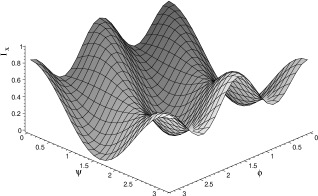
Figure 2: $I_{x}$, for a normal incidence angle and for the plate thickness $\ell_{1}$, as a function of the angles $\phi$ and $\psi$ (in radian). The optical axis is parallel to the plane of interface.

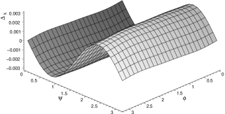
Figure 3: $\Delta_{x}$, for a normal incidence angle and for the plate thickness $\ell_{1}$, as a function of the angles $\phi$ and $\psi$ (in radian). The optical axis is parallel to the plane of interface.

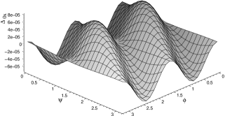
Figure 4: $\Delta_{0x}$, for a normal incidence angle and for the plate thickness $\ell_{1}$, as a function of the angles $\phi$ and $\psi$ (in radian). The optical axis is parallel to the plane of interface.

The previous discussion holds for quarter wave plates. Let us consider another plate thickness $\ell_{3}=1018.49\mu$m, i.e. a fourteen order half wave plate. $I_{x}$, $\Delta_{x}$ and $\Delta_{0x}$ are shown as a function of $\phi$ and $\psi$ in Figs. 5, 6 and 7 respectively. The effect induced by the optical activity is here reduced by two orders of magnitude with respect to a quarter wave plate and is dominated by the variation of the phases $\varphi_{o}$ and $\varphi_{e}$ with $g_{11}$. For a first order half wave plate ($\ell_{4}=105.36\mu$m), the effect on $\Delta_{0x}$ is reduced by an order of magnitude whereas $\Delta_{x}$ is essentially unchanged.

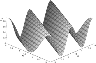
Figure 5: $I_{x}$, for a normal incidence angle and for the plate thickness $\ell_{3}$, as a function of the angles $\phi$ and $\psi$(in radian). The optical axis is parallel to the plane of interface.

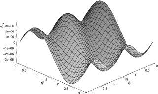
Figure 6: $\Delta_{x}$, for a normal incidence angle and for the plate thickness $\ell_{3}$, as a function of the angles $\phi$ and $\psi$ (in radian). The optical axis is parallel to the plane of interface.

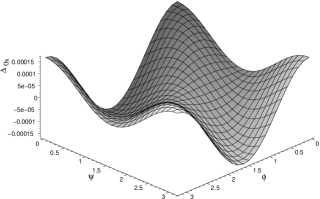
Figure 7: $\Delta_{0x}$, for a normal incidence angle and for the plate thickness $\ell_{3}$, as a function of the angles $\phi$ and $\psi$ (in radian). The optical axis is parallel to the plane of interface.

As mentioned in section 3.1, under normal incidence and for the optical axis parallel to the plane of interface, the contribution of the optical activity to the platelet transmission matrix comes essentially from the coefficient $g_{11}$. The contribution of the coefficient $g_{33}$ appears under oblique incidence and can, a priori, be distinguished from the other one by considering various angles of incidence. We now consider the ratio $r=I_{s}/I_{p}$ where $I_{s}$ and $I_{p}$ are obtained by substituting ${\rm\bf\hat{s}}$ and ${\rm\bf\hat{p}}$ to ${\rm\bf\hat{x}}$ in Eq. (40) respectively. To reproduce the experimental results of Ref. [6], we also fix $\psi=\pi/4$, i.e. $\mbox{${\rm\bf E_{in}}$}=(1,1)^{T}/\sqrt{2}$. The ratio $r$ is shown as a function of $\phi$ and $\theta$ for the plate thickness $\ell_{1}$ in Fig. 8. To distinguish the contributions from $g_{11}$ and $g_{33}$, we show in Figs. 9 and 10 the relative differences $\delta r=(r-r_{0})/r$ and $\delta^{\prime}r=(r-r_{1})/r$ where $r_{0}$ and $r_{1}$ are obtained by setting $g_{11}=g_{33}=0$ and $g_{11}=0$ in the expression of $r$ respectively. From these figures, one sees that, as reported in Ref. [6], the contribution of the optical activity reach the percent level for certain values of $\phi$.

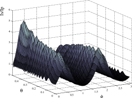
Figure 8: $r$ as a function of the angles $\theta$ and $\phi$ (in radian) for an incident electric vector $\mbox{${\rm\bf E_{in}}$}=(1,1)^{T}/\sqrt{2}$ and for the plate thickness $\ell_{1}$. The optical axis is parallel to the plane of interface.

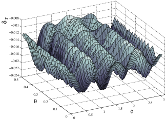
Figure 9: $\delta r$ as a function of the angles $\theta$ and $\phi$ (in radian) for an incident electric vector $\mbox{${\rm\bf E_{in}}$}=(1,1)^{T}/\sqrt{2}$ and for the plate thickness $\ell_{1}$. The optical axis is parallel to the plane of interface.

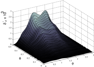
Figure 10: $\delta^{\prime}r$ as a function of the angles $\theta$ and $\phi$ (in radian) for an incident electric vector $\mbox{${\rm\bf E_{in}}$}=(1,1)^{T}/\sqrt{2}$ and for the plate thickness $\ell_{1}$. The optical axis is parallel to the plane of interface.

In addition, we observe here that the contribution of $g_{33}$ is negligible under normal incidence but reaches the few $10^{-3}$ level for reasonable values of the angle of incidence. The shape of the contribution of $g_{11}$ and $g_{33}$ being different, it seems possible to determine both coefficients by measuring $r$ as a function of $\phi$ for various angles of incidence.

We finally consider the case of an optical axis perpendicular to the plane of interface. We choose $\ell_{5}=1000\mu$m for the plate thickness and, as previously, $\mbox{${\rm\bf E_{in}}$}=(1,1)^{T}/\sqrt{2}$ for the incident electric vector. In addition to $\delta r$, we introduce the phase angle $\alpha$ defined by the argument of the complex number $(\mbox{${\rm\bf E_{out}}$}\cdot\mbox{${\rm\bf\hat{s}}$})/(\mbox{${\rm\bf E_{out}}$}\cdot\mbox{${\rm\bf\hat{p}}$})$ and the difference $\Delta\alpha=\alpha-\alpha_{0}$ where $\alpha_{0}$ is obtained by setting $g_{11}=0$ in the expression of ${\rm\bf E_{out}}$. Figs. 11 and 12 show $\delta r$ and $\Delta\alpha$ as a function of the angle of incidence $\theta$.

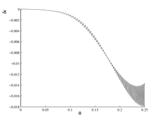
Figure 11: $\delta r$ as a function of the angle $\theta$ (in radian) for an incident electric vector $\mbox{${\rm\bf E_{in}}$}=(1,1)^{T}/\sqrt{2}$ and for the plate thickness $\ell_{5}$. The optical axis is perpendicular to the plane of interface.

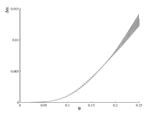
Figure 12: $\Delta\alpha$, in radians, as a function of the angle $\theta$ (in radian)for an incident electric vector $\mbox{${\rm\bf E_{in}}$}=(1,1)^{T}/\sqrt{2}$ and for the plate thickness $\ell_{5}$. The optical axis is perpendicular to the plane of interface.

As in the case of an optical axis parallel to the plane of interface, the measurements of $r$ and $\Delta\alpha$ as function of the angle of incidence lead to the determination of both $g_{11}$ and $g_{33}$. The sensitivity to these parameters is even higher when the optical axis is perpendicular to the plane of interface.

5 Conclusion

The transmission matrix for a uniaxial and chiral platelet has been calculated for an optical axis parallel and perpendicular to the plane of interface. The optical activity has been taken into account by considering the electric- quadrupole and magnetic-dipole responses of the crystal medium. Simple and usable expressions have been derived for normal incidence and for the optical axis parallel and perpendicular to the plane of interface. The case of an oblique incidence has been treated partly analytically and partly numerically.

As an application, numerical studies of the transmission of quartz platelets of various thicknesses have been provided. Under normal incidence, it was shown that the contribution of the optical activity can reach the percent level for quarter wave plates, independently of the plate’s order. Such a high contribution was found to be due to the transmission and reflection interface matrices. The case of half wave plates was also investigated and, unlike quarter wave plates, the main contribution of the optical activity came from the phase shift induced by the optical path inside the crystal. The variation of the intensity after a quartz platelet was studied as a function of the angle of incidence and of the orientation of the optical axis. A sensitivity to both gyration coefficients $g_{11}$ and $g_{33}$ was observed under oblique incidence. This suggests that varying the angle of incidence one could determine experimentally these two coefficients with a unique crystal cut. With respect to the results of Ref. [22], oblique incidence also offers the possibility to determine very accurately the platelet thickness and thereby the gyration coefficients.

References

• [1] E.U. Condon, Rev. Mod. Phys. 9 (1937) 432.
• [2] J.F. Nye, Physical properties of crystals, Oxford University Press, Oxford, 1985.
• [3] I. Scierski and F. Ratajczyk, Optik 68 (1984) 121.
• [4] K. Pietrasszkiewicz, W.A. Wozniak and P. Kurzynowski, J. Opt. Soc. Am. A12 (1995) 420.
• [5] O.S. Kushnir, J. Phys.: Condens. Matter 8 (1996) 3921.
• [6] C. Chou, Y.-C. Huang and M. Chang, J. Opt. Soc. Am. A14 (1997) 1367.
• [7] P. Gomez and C. Hernandez, J. Opt. Soc. Am. B15 (1998) 1147.
• [8] A. Yariv and P. Yeh, Optical waves in crystals, John Wiley and Sons, New-York, 1984.
• [9] M.P. Silverman and J. Badoz, J. Opt. Soc. Am. A7 (1990) 1163.
• [10] A.I. Miteva and I.J. Lalov, J. Phys.: Condens. Matter 5 (1993) 6099.
• [11] E.B. Graham and R.E. Raab, Proc. R. Soc. Lond. A 430 (1990) 593.
• [12] R.E. Raab and J.H. Cloete, J. Electromagn. Waves Appl. 8 (1994) 1073.
• [13] E.B. Graham and R.E. Raab, J. Opt. Soc. Am. A13 (1996) 1239.
• [14] P. Yeh, J. Opt. Soc. Am. 72 (1982) 507.
• [15] R.R. Birss, Symmetry and magnetism, North-Holland Publishing Company, Amsterdam, 1964.
• [16] P. Yeh, J. Opt. Soc. Am. 69 (1979) 742.
• [17] T.D. Wen, Y.S Raptis, E. Anastassakis, I.J. Lalov and A.I. Miteva, J. Phys. D: Appl. Phys. 28 (1995) 2128.
• [18] A.I. Miteva, I.J. Lalov, T.D. Wen, Y.S Raptis and E. Anastassakis, J. Phys. D: Appl. Phys. 29 (1996) 2705.
• [19] K. Zander, J. Moser and H. Melle, Optik 70 (1985) 6.
• [20] S. Bassiri, C.H. Papas and N. Engheta, J. Opt. Soc. Am. A5 (1988) 1450.
• [21] R.B. Sosman, The properties of silica, Chem. Catalog Co., New- York, 1927.
• [22] J. Poirson, T. Lanternier, J.-C. Cotteverte, A.L. Floch and F. Bretenaker, Appl. Opt. 34 (1995) 6806.