Synchronization of organ pipes: experimental observations and modeling

Abstract

We report measurements on the synchronization properties of organ pipes. First, we investigate influence of an external acoustical signal from a loudspeaker on the sound of an organ pipe. Second, the mutual influence of two pipes with different pitch is analyzed. In analogy to the externally driven, or mutually coupled self-sustained oscillators, one observes a frequency locking, which can be explained by synchronization theory. Further, we measure the dependence of the frequency of the signals emitted by two mutually detuned pipes with varying distance between the pipes. The spectrum shows a broad “hump” structure, not found for coupled oscillators. This indicates a complex coupling of the two organ pipes leading to nonlinear beat phenomena.

PACS numbers: 05.45.Xt, 47.52.+j, 43.75.+a, 43.28.+h

I Introduction

Sound production in organ pipes is traditionally described as a generator-resonator coupling. In the last decades, research has been concerned with the complex aeroacoustic processes which lead to a better understanding of the sound generation in a flue organ pipe. The process of sounding a flue-type organ pipe employs an airstream directed at an edge, the labium of an organ pipe. An oscillating “air sheet” is used to describe the situation in which the oscillations of the jet exiting from the flue are responsible for the creation of the pipe sound Fabre-00 ; RossingFletcher-97 . Using the “air sheet” terminology, it is pointed out that the oscillation is controlled not by pressure, as in earlier investigations Cremer-Ising-68 ; Coltman-68 ; Coltman-92ab ; Fletcher-93 ; Nolle-83 , but by the air flow Coltman-76 ; Verge-94 ; Verge-97a ; Verge-97b ; Fabre-Hirschberg-96 ; Segoufin-04 .

The situation becomes more involved if two flue organ pipes are close in sounding frequency and in spatial distance. Then a synchronization of the pipes, a frequency locking, occurs Rayleigh2-45 ; Bouasse-29 ; Stanzial-00 ; Angster-93 . This has a direct importance for the arrangement of organ pipes in a common Orgelwerk. The effect has been known by organ builders for a long time and taken into account intuitively in the design of organs Schuke-private . Some measurements of the acoustic field or of its dependence on the mutual coupling or on the distance between the pipes have been reported first in the early 20th century Bouasse-29 , but no theoretical explanation was given. In this article, we report acoustic measurements and give a possible explanation by means of modern synchronization theory Pikovsky-Rosenblum-Kurths-01 . To a certain approximation, an organ pipe can be considered as a self-sustained oscillator, explained in detail below. In this context, the synchronization of a pipe by an external, acoustical force is important, such that we carried out additional measurements, where a pipe stands aside a loudspeaker whose frequency is tuned around the pipes pitch. As well in this case, the pipe is found to be synchronized.

As a side result of these measurements, we can clarify a discussion about the nature of the strong amplitude decrease for two coupled pipes, already observed by Lord Rayleigh Rayleigh2-45 and later by very detailed measurements of Bouasse Bouasse-29 . As a possible interpretation, the so-called oscillation death has been given in Pikovsky-Rosenblum-Kurths-01 , which means that there is an oscillation breakdown at the the pipe mouth, and all the energy is dissipated. From our results, we rule out such a scenario and suggest an antiphase oscillation which yields destructive interference of the emitted acoustic waves. This holds for two neighboring pipes, as well as for the pipe standing aside a loudspeaker.

This article is structured as follows: In section II we explain briefly the generation of sound in an organ pipe and review basic concepts from synchronization theory. In section III we report on detailed measurements of the synchronization of a loudspeaker positioned directly on the side of a pipe and observe two adjacent pipes. The results are interpreted within the frame of synchronization theory. We give an explanation of why a model of two oscillators works out so well, as indicated in Stanzial-00 . Further, the dependence of the frequency spectrum on the distance between two detuned pipes is investigated for a fixed amount of detuning. Finally, we conclude with section IV.

II Basic principles

A Sound generation in organ pipes

Sound generation in organ pipes has been repeatedly investigated Coltman-76 ; Fabre-Hirschberg-96 ; Rayleigh-82 . Here, the beauty of musical sound generation is paired with complex aerodynamical phenomena; their coupling to the acoustic field has been understood to a reasonable degree in the last 30 years (see the review Fabre-00 ).

Let us consider a single organ pipe: The wind system blows with constant pressure producing a jet exiting from the pipe flue. Typical Reynolds numbers, corresponding to a free jet are of the order of $10^{3}$, depending on the pressure supplied and the pipe dimensions, see Fabre-Hirschberg-96 ; Pitsch-Angster . The jet exiting from the flue generates a pressure perturbation at the labium of the pipe which travels inside the pipe resonator and is reflected at the end of the resonator. This pressure wave returns after time $T$ to the labium where it in turn triggers a change of the phase of the jet oscillations. After a few transients, a stable oscillation of an “air sheet” at the pipe mouth is established. This oscillation of the wind field couples to the acoustic modes and a sound wave is emitted. Thus, the system can be considered as a damped linear oscillator (the resonator) which controls the periodic energy supply of the air-jet by the air column oscillation. We want to adapt this idea of an organ pipe as a self-sustained oscillator Fletcher-79 ; Fletcher-99 to understand the mechanism of mode- or frequency locking Fletcher-78 , or synchronization.

One feature of a self sustained oscillator is the occurence of oscillations even for constant driving. The physical mechanism is the balance of energy losses and energy input. The classical example is the van der Pol oscillator (Fig. 1), where a Triode (or more modern, a tunnel diode) acts as “negative resistance” whose response is fed back to an electrical oscillator. In the case of an organ pipe, energy is supplied by the wind system, losses are due to internal dissipation in the spatially extended resonator, and radiation. The negative resistance is represented by the air stream at the pipe mouth and the feedback coupling is given by the boundary conditions between the “air sheet” wind field and the air-column oscillations in the resonator. It can be described by impedances Fletcher-76 , detailed results for two coupled Helmholtz resonators are given in Johansson-Kleiner-01 . Of course, the exact form of the limit cycle and thus the acoustic oscillations depend on the details of energy losses, as the quality factor of the resonators, the radiation of sound, and the understanding of the energy supply by the coupling to the jet. The general mechanism, however, remains untouched, since only a nonlinear growth of losses and supply is needed for a self-sustained oscillator to work. Here, we do not want to investigate these details, but rather emphasize the general character of our investigations.

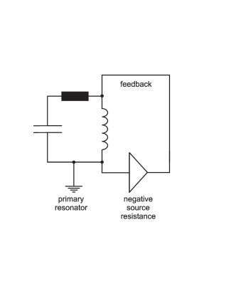
\psfrag{Yaxis}{\small$\dot{x}$}\psfrag{Xaxis}{\small$x$ }\includegraphics[width=173.44534pt]{fig2.eps}

Figure 1: Left:Schematic diagram for a self sustained oscillator. Right: resulting limit cycle behavior.

The sound emitted by this complex system can be evaluated by the coupling of the flow and the acoustic modes in the framework of aeroacoustic modeling on the basis of Lighthills analogy. According to Howe Howe-75 ; Howe-03 ; Howe-98 , the sound generation is dominated by the singularity at the edge of the labium. Numerical approaches still suffer from the very expensive runs needed to resolve the large range of excited scales and the proper choice of boundary conditions Lele-97 ; Tam-97 .

B Synchronization of self-sustained oscillators

In his book, Lord Rayleigh states “When two organ pipes of the same pitch stand side by side … it may still go so far as to cause the pipes to speak in absolute unison in spite of inevitable small differences” Rayleigh2-45 . He describes the so-called “Mitnahme-Effekt” (loosely the take-along effect), known by organ builders Stanzial-00 ; Angster-93 . In Pikovsky-Rosenblum-Kurths-01 the phenomenon is interpreted in the frame of synchronization theory. Hereafter we will use the terms frequency locking or synchronization to be synonymous with the “Mitnahme-Effekt”. In Angster-93 , the effect has been analyzed heuristically, while Stanzial has investigated the dependence of the frequency locking on the detuning or frequency difference of two single pipes in Stanzial-00 by acoustic measurement. He modeled the effect by two coupled oscillators, without giving a physical reason of the coupling. A treatment of the mode-locking phenomenon, specific for musical instruments is very nicely given in Fletcher-99 . In the following we will rely on synchronization theory to show that any self-sustained coupled oscillator generically shows synchronization.

Probably the most important feature of self-sustainment is the occurrence of an attracting limit cycle. It appears due to two properties: nonlinearity, and the energy balance between losses and driving. For a linear, damped oscillator a limit cycle solution does not exist, the only possible attractor is the trivial solution. Nonlinearity allows for the dependence of frequency on amplitude which constitutes a mechanism to drive the system towards an amplitude at which the regular oscillations are established. Since the amplitude corresponds directly to the mechanical energy of the system, this is right at the point of equality of losses and supply – the limit cycle.

We want to sketch the principles for synchronization of an oscillator with an external driving and then explain the interaction of two oscillators. In the following we will discuss some equations in terms of the angular frequencies and return later to frequencies when the measurements are concerned.

A Single Oscillator: Let us consider the equation for a harmonic oscillator with negative, nonlinear resistance:

$$\ddot{x}=-\omega_{0}^{2}x-\frac{d}{dt}f(x)=-\omega_{0}^{2}x-\dot{x}\frac{df}{dx}\;,$$ (1)

where $\omega_{0}$ is the angular frequency of the harmonic system and $f(x)$ is a nonlinear function with at least one part of positive and another part of negative slope. Now we discuss the basic principles by the concrete example of the van der Pol oscillator and give general results without further derivation, for details see Pikovsky-Rosenblum-Kurths-01 . In the case of the van der Pol oscillator $f(x)=\alpha x-\frac{1}{3}\beta x^{3}$, and $\omega_{0}^{2}=(LC)^{-1}$. The energy supply is accounted for by $\alpha$, the losses by $\beta$. If the inharmonicity is not too great, the amplitude on the limit cycle differs little from the harmonic oscillator and the phase coincides approximately with the harmonic one. To get rid of fast oscillations, one applies the method of averaging Bogoliubov-Mitropolsky-61 : One inserts for the amplitude $x(t)=A(t)\sin(\Theta_{0})=A(t)\sin(\omega_{0}t)$ and collects terms of the different time scales 1 and $\omega_{0}$. So, one obtains an equation for the slowly varying amplitude $A(t)$, and for the phase $\Theta_{0}$ here for the van der Pol oscillator.

$$\dot{A} = 1/2\left(\alpha-\frac{1}{4}\beta A^{2}\right)A\;,$$ (2)

$$\dot{\Theta}_{0} = \omega_{0}\;.$$ (3)

Eq. 3 describes the slow relaxation of the amplitude towards the steady state. A limit cycle exists for $|A|^{2}=\frac{4\alpha}{\beta}$. The solution of the phase equation allows for the addition of an arbitrary constant phase. Thus, one can shift the state along the cycle without changing the energy. This allows for the adjustment of the phase, when the system is driven, or coupled to another oscillator. This adjustment is exactly what we understand as synchronization, or mode-locking.

A Driven, Single Oscillator: If the system is driven externally by a harmonic force with angular frequency $\omega_{1}\simeq\omega_{0}$, two time scales are present in the system, a fast one $t_{f}=\frac{2\pi}{\omega_{1}}\simeq=\frac{2\pi}{\omega_{0}}$, and a slow one $t_{s}=\frac{2\pi}{\omega_{1}-\omega_{0}}$, and $t_{s}\ll t_{f}$. The corresponding equation

$$\ddot{x}+\omega_{0}^{2}x-\dot{x}\frac{df}{dx}=\omega_{1}^{2}R\cos(\omega_{1}t)\;,$$ (4)

We want to investigate now the dependence on the slow time and average over the fast one. To do so, we use the ansatz $x(t)=A(t)\sin(\omega_{1}t+\phi)$, with $\phi$ the slow phase (It is a bit easier working with a complex amplitude, substituting $x=Ae^{i\omega_{1}t+\phi},\;\dot{x}=A\omega_{1}e^{i\omega_{1}t+\phi}$). By using again the averaging method one obtains after a few straightforward steps Landa-96 ; Pikovsky-Rosenblum-Kurths-01

$$\dot{a} = \frac{1}{2}\left(\alpha-\frac{1}{4}\beta a^{2}\right)a-\frac{\omega_{1}R}{2}\cos\phi\;,$$ (5)

$$\dot{\phi} = \frac{1}{2}\frac{\omega_{0}^{2}-\omega_{1}^{2}}{\omega_{1}}+\frac{\omega_{1}}{2}\frac{R}{a}\sin\phi\;.$$ (6)

The second equation is known as the Adler equation Adler-46 ; Pikovsky-Rosenblum-Kurths-01 ; the general form for the phase equation depends on the nonlinear function $f(x)$ and can be seen as the difference of the equations for the two fast variables $\omega_{1}$, and $\omega_{0}$:

$$\begin{array}[]{lcl}\dot{\Theta}_{1}&=&\omega_{1}\;,\\ \dot{\Theta}_{2}&=&\omega_{0}+\epsilon q(\omega_{0}-\omega_{1})\;,\end{array}\hskip 17.22217pt\dot{\phi}=\dot{\Theta}_{2}-\dot{\Theta}_{1}=\Delta\omega+\epsilon q(\phi)$$ (7)

with a $2\pi$-periodic function $q$, and the two parameters detuning $\Delta\omega=\frac{1}{2}\frac{\omega_{0}^{2}-\omega_{1}^{2}}{\omega_{1}}\simeq\omega_{0}-\omega_{1}$ and locking term $\epsilon=\frac{\omega_{1}}{2}\frac{R}{a}$, which is proportional to the driving strength. To zero order, one can assume $a\simeq const$and the phase equation effectively decouples from the amplitude equation, which in turn is driven by the phase, similar holds for a first order Pikovsky-Rosenblum-Kurths-01 . The Adler equation ($q(\phi)=\sin(\phi)$) has two stationary solutions, $\dot{\phi}=0$, for $|\Delta\omega|\leq\epsilon$. The stability of these fixed points, $\phi_{s}$ and $\phi_{u}$, is determined by linear stability analysis. One puts $\phi=\phi_{s/u}+\delta\phi$, inserts this expression into (7) and Taylor-expands the expressions. The stable point is given by $\cos\phi_{s}<0$, the unstable one by $\cos\phi_{u}>0$, corresponding to exponential decay or growth of the perturbation $\delta\phi$. In general, if higher harmonics enter in $q(\phi)$ several fixed points can exist and the positions can be strongly asymmetric, cf. Fig. 2.

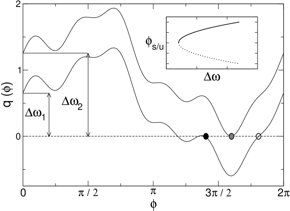
Figure 2: Stable (filled circle) and unstable (open circle) fixed point $\Theta_{s}$, $\Theta_{u}$ for the Adler equation to illustrate the mode locking. If detuning or coupling is varied, the phase is adjusted accordingly by the system to the stable fixed point. For $\Delta\omega-\epsilon=0$ both fixed points merge; this results in a saddle-node bifurcation, as sketched in the inset; the straight/dotted line corresponds to the stable/unstable fixed point.

The transition to synchronization: If one varies the detuning from zero to $\epsilon$ the phase varies from zero to (at most) $\pi$. At the merging -, or bifurcation point, $\Delta\omega_{max}-\epsilon=0$, and the stable and unstable fixed point annihilate (opaque in Fig. 2). This type of bifurcation is known as saddle-node bifurcation Ott-94 . In the case of an unstable saddle one attracting and one repelling direction to/from the periodic limit cycle exist, for a stable cycle two attracting directions exist, as for a stable node.

Inside the synchronization region, the phase difference $\phi=\phi_{0}=const$, and the phase of the observed oscillation is $\omega_{1}t+\phi_{0}$. Let us turn to the phase dynamics outside the synchronization region. For $\dot{\phi}\neq 0$, one can formally integrate Eq.(7) to obtain

$$t=\left|\int_{\phi_{0}}^{\phi}\frac{d\phi^{\prime}}{\epsilon q(\phi^{\prime})-\Delta\omega}\right|$$ (8)

The period $T=2\pi/\omega_{b}$ results with the integration bound $\phi=\phi_{0}+2\pi$. The total phase rotates uniformly $\varphi=\omega_{1}t+\phi(t)=\omega_{1}t+\omega_{b}t=\Delta\Omega t$ and one recognizes the typical beat phenomenon, as for the superposition of two harmonic waves; only that here the beating is strongly nonlinear. For harmonic oscillations the phase-slip of the beating is distributed over the whole interval. Close to the bifurcation from the synchronized region, one observes long epochs of nearly constant phase $\phi\simeq\phi_{max}$ broken by relatively short intervals in which the phase rotates by $2\pi$. We observe this behavior as well for coupled organ pipes, this is illustrated below by a plot of the measured time signal close to the synchronized region.

For a saddle-node bifurcation, one expects a square root dependence of $\Delta\Omega$ on the detuning $\Delta\omega$. This indeed by expansion of the denominator in (8):

$$|\Delta\Omega| \simeq 2\pi\left|\int_{-\infty}^{\infty}\frac{d\phi}{\epsilon/2q^{\prime\prime}(\phi_{max})\phi^{2}-(\Delta\omega-\Delta\omega_{max})}\right|^{-1}\;,$$ (9)

$$= \sqrt{\epsilon|q^{\prime\prime}(\phi_{max})|\cdot(\Delta\omega-\Delta\omega_{max})}\simeq\sqrt{\Delta\omega-\Delta\omega_{max}}$$ (10)

A very detailed description, including many examples and generalizations is given in Pikovsky-Rosenblum-Kurths-01 .

Two coupled oscillators: Now, we will turn our attention to the case of two oscillators and focus to the equations for the phases. From the above, it is now clear that any pair of uncoupled, self-sustained oscillators close to a limit cycle can be written in terms of phase, ($\Theta_{1},\Theta_{2}$), and amplitude, ($A_{1},A_{2}$), in the following form:

$$\dot{\Theta}_{i} = \omega_{i}$$ (11)

$$\dot{A_{i}} = -\gamma\,(A_{i}-A_{i,0})\,,$$ (12)

with $i=1,2$. For weak coupling, one can again perform an expansion and apply the method of slowly varying amplitude such that the phase equations are, analogous to (7)

$$\dot{\Theta}_{1} = \omega_{1}+\epsilon G_{1}(\Theta_{1},\Theta_{2})\;,$$ (13)

$$\dot{\Theta}_{2} = \omega_{2}+\epsilon G_{2}(\Theta_{1},\Theta_{2})\;.$$ (14)

For $\omega_{1}\simeq\omega_{2}$ the phase difference $\phi=\Theta_{1}-\Theta_{2}$ is a slow variable. The discussion can now follow the above, with the difference that now the oscillators have to adjust themselves mutually, whereas above one oscillator adjusted its frequency to an external driving.

We have to distinguish very carefully and clearly between the single angular frequencies $\omega_{i}$, measured for a decoupled system, and the angular frequencies $\dot{\Theta}_{i}$ measured for the coupled system. For a clear nomenclature, we call the difference of the uncoupled frequencies detuning, and denote it by the symbol $\Delta f=(2\pi)^{-1}(\omega_{2}-\omega_{1})$. The frequency difference of the coupled system is always denoted by $\Delta\nu$. A typical plot visualizes $\Delta\nu$ against the detuning $\Delta f$. One observes a plateau $\Delta\nu=0$ for a synchronized region and a linear dependence for uncoupled oscillations. Below, we will use the symbol $f$ for uncoupled frequencies, and $\nu$ for measurements of the coupled pipes, analogously we use $\Delta f$ and $\Delta\nu$.

At the end of this section, we would like to hint to two facts: i) the theory presented above holds only for small deviations from harmonic oscillations and for small coupling. For large parameters, in principal the considerations still hold, but quantitatively deviations are expected. ii) Even though it seems appealing to explain the frequency locking of organ pipes in such a simple way, it is not completely satisfactory because organ pipes are extended systems and such a simple description does not take into account the aeroacoustics which is eventually needed for a complete understanding.

III Measurement and Results

A Measurement Setup and Signal Analysis

Table 1: Pipe geometry.

pipe-body
overall length (without foot)	530 mm
clear length (adjustable)	$370\ldots 450\,\mathrm{mm}$
wall thickness	$6\,\mathrm{mm}$
cross section
shape	quadratic
clear width	37 mm
clear depth	48 mm
mouth
cut-up height	7 mm
cut-up width	37 mm
flue-exit height	0.4 mm
foot
length	320 mm
toe hole diameter	15 mm

Measurements were carried out on a miniature organ especially made by Alexander Schuke GmbH for physical investigations. Just like a real organ it consists of a blower connected by a mechanical regulating-valve to the wind-belt and finally a wind-chest upon which the pipes are positioned. Since only stationary behavior was of interest we joined the two pipes directly to the wind-belt with flexible tubes. The wind pressure was set by the organ builder to a mean value of 160 Pa. Over 10 s we measured a standard deviation value of 6 Pa in the pipe foot. The wind may be considered as very stable.

The pipes used are stopped, a detailed description of the pipe-geometry is given in table 1. The resonator top of the pipes was movable in order to adjust resonator-length and pitch. To minimize losses, a gasket made of felt was applied. The pipes as delivered from the manufacturer were tuned to e and f in German notation, that is E3 and F3 in American notation. The applied driving pressure roughly yields a Reynolds number $Re=435$.

The acoustic signal was measured by a B&K 4191 condenser microphone positioned at the centerline between the sound sources. Further information on positioning of the acoustic sources and the microphone is given in sections B and C. Measurements took place inside the anechoic chamber of the Technical University of Berlin. The rooms size is $W\cdot L\cdot D=20\,\mathrm{m}\cdot 17\,\mathrm{m}\cdot 7\,\mathrm{m}$ giving a volume of $2000\,\mathrm{m^{3}}$. The low cut-off frequency of this room is 63 Hz. Temperature, humidity and pressure conditions were kept stable to keep there influence on the measurements negligible.

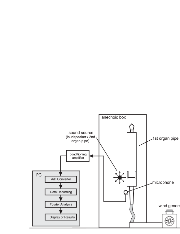
Figure 3: Sketch of the experimental setup. The microphone is in plane with the pipe mouth, the view is at an angle from above.

The recording of the sensor signal as a function of time was achieved via hard-disk recording with a M-Audio 2496 Soundboard at a sampling rate of 44.1 kHz and a resolution of 16 bit and saved in PCM format. Data analysis was performed with Matlab. All Spectra shown in the results are Fourier transformed out of 10 s (441 000 samples) of time signal, giving a frequency-resolution of 0.1 Hz. During Fourier transformation a symmetric Hann window was applied to time data. All spectra have been averaged. From these spectra the amplitude of the harmonics was read out by a routine searching for the maximum signal level within a frequency range of $\pm 0.3\,\mathrm{Hz}$.

B Organ Pipe driven externally by a Loudspeaker

To investigate the influences of a external sound source onto the organ-pipe we positioned ax loudspeaker directly beside a single organ-pipe. The loudspeaker was a 2-Way Active System MS 16 from Behringer. The woofers cone-diameter is 10 cm. The speaker was connected to a HP 33120A waveform generator, delivering a sinusoidal signal. The sound pressure level emitted by the loudspeaker was set equivalent to the volume of the fundamental organ tone within $81.5\pm 0.25\,\mathrm{dB}$. At this level the distortion of the speaker was at THD=1.5%. The experiment started with the pipe at a fundamental frequency of 168.3 Hz and the loudspeaker at 165.8 Hz. During the measurement the organ-pipe remained unchanged but the frequency of the loudspeaker was very slowly, every 40 seconds, increased by 0.1 Hz. This gives the possibility to average ten seconds of signal four times to suppress noise. The microphone was positioned at the centerline between pipe and loudspeaker at a distance of 15 cm. A picture of the setup is given in Fig. 4.

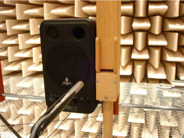
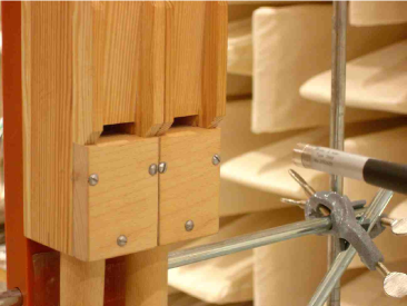
Figure 4: Fotograph of the measurement setup. Left: loudspeaker and pipe sounding together, right: two “coupled” organ pipes

The synchronization can be observed clearly by the plateau in the plot of frequency difference, $\Delta\nu$ against detuning, $\Delta f$. As well the predicted square root function is observed at the transition to synchronization, cf. Fig. 5. The amplitude recorded with the microphone shows a positive and negative peak, at the beginning and end of the synchronization, respectively. Invoking the explanations of synchronization theory, cf. Eq. 7, this amounts to a change of the relative phase from 0 to $\pi$. If loudspeaker and pipe are considered as monopole sources, their field at the centerline, where the signal is recorded, can be obtained as a superposition of two fields with equal, measured amplitude and phase difference $\phi_{0}$, decaying as $1/r$: $A(r)=A_{0}/r+A_{0}/{r}\cos\phi_{0}$ (remember that we adjusted the sound pressure level of loudspeaker and pipe, so $A_{speaker}=A_{pipe}=A_{0}$). For $\phi_{0}=0$ interference is positive, $\phi_{0}=\pi$ implies negative interference. This is exactly seen in Fig. 5b, where we plot the peak amplitude of the loudspeakers frequency (open circle), and the first harmonic of the organ pipe (filled circles), respectively, over the detuning. For zero detuning, $\phi_{0}=\pi/2$. This corresponds to an interval of $\pi$ within the synchronization region; i.e. from positive to negative superposition. One notices that the phase $\phi_{0}=\pi/2$ right at $A=A_{0}$. This corresponds to an equal distribution of energy at this point. The increase of the amplitude at the loudspeakers frequency at the left hand of the synchronization region comes from the above mentioned effect that the pipe sounds for long periods with the frequency of the speaker to undergo a fast phase slip, when close to be synchronized. This results in a higher peak amplitude at the loudspeakers frequency (cf. the discussion in Sec. D).

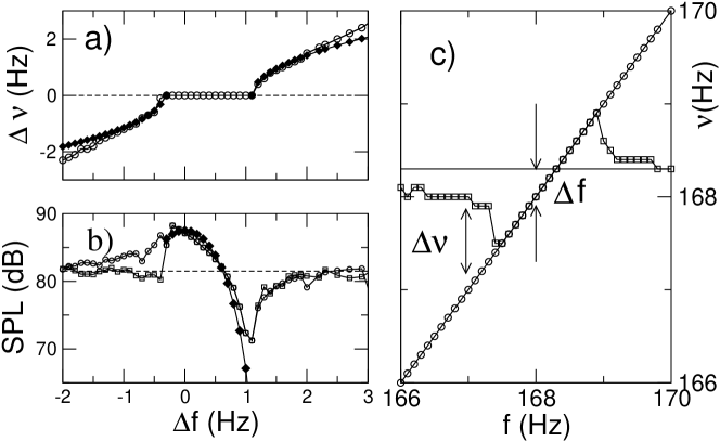
Figure 5: Upper left (a): Frequency locking of organ pipe and loudspeaker. Top: observed frequency difference $\Delta\nu$ ascertained with pipe and loudspeaker sounding together versus detuning $\Delta f$ (open circles). In the synchronization region, a very clean plateau is observed. A saddle-node bifurcation (filled diamonds) occurs at the edges, as predicted by Eq. (9). Bottom left (b): Measured amplitude signal in dB. The phase varies from $0$ to $\pi$ over the synchronization plateau. The region is asymmetric; $\Delta\nu\in(-0.3,1.1)$ within the frequency resolution. The circles indicate the peak amplitude at the loudspeakers frequency, and the pipes frequency (squares). The superposition of the signals including the phase shift along the plateau is plotted by filled diamonds, the agreement is quite good. Right (c): absolute measured signals for pipe and loudspeaker sounding together ($\nu$, open circles) and the signals for speaker alone (squares) and pipe alone (straight line). The detuning is indicated by $\Delta$f, as the difference of the “uncoupled oscillators”, pipe and speaker alone; the frequency difference, $\Delta\nu$ results from the subtraction of the measured signal for pipe and speaker sounding simultaneously, coupled and the varied frequency, in our case of the loudspeaker.

C Two Pipes standing side by side

To measure the dependence of frequency locking on the detuning of the two pipes, both pipes were installed on a common bar directly side by side (see Fig. 4. One of the pipes has been kept at the fixed frequency of $170.1Hz$, the other pipe was detuned in variable steps. With two pipes connected to the wind-chest one cannot detect the fundamental frequency of one pipe by simply turning of the other through closing the pipes valve. This would raise the wind pressure for the investigated pipe and consequently also the frequency itself. In order to acquire the value precisely the pipe at a fixed frequency was made soundless by putting a little absorber-wedge into the mouth. Doing so the air–sheet oscillation and therefore sound generation is suppressed, but the air consumption remains the same, keeping the wind-pressure stable.

In Stanzial-00 , the frequencies $\nu_{1}$, $\nu_{2}$ of the coupled pipes were plotted against the frequency detuning of the uncoupled pipes, $\Delta f$. As explained above, a clearer characterization is achieved when the frequency difference $\Delta\nu$ is plotted versus $\Delta f$ Bogoliubov-Mitropolsky-61 ; Pikovsky-Rosenblum-Kurths-01 . We plot this quantity in Fig. 6. Clearly, the typical behavior of frequency locking can be observed. As synchronization theory predicts, the bifurcation close to the ends of the locking region is of saddle node type Ott-94 (filled diamonds in Fig. 6a).

Now, stressing the analogy with two coupled oscillators, a change of the relative phase from $\phi_{0}-\pi/2$ to $\phi_{0}+\pi/2$ is expected Pikovsky-Rosenblum-Kurths-01 ($\phi=2\pi f$). This has consequences for the amplitude of the emitted sound. The radiated sound wave in the far field can be roughly approximated by a spherical wave, and the field at the measurement point $\vec{r}$ is obtained by superposition of the two waves emitted at the pipe mouths positions. Assuming the sources to be point-like and considering that the pipes are situated directly side-by-side, the amplitude along the center line is $A={2A_{0}}/{r}\,(1+\cos\phi_{0})$, this has already been described in Bouasse-29 . The notation is as above, please note that here $A_{pipe1}=A_{pipe2}=A_{0}$, because both pipes have approximately the same amplitude, cf. Fig. 6.

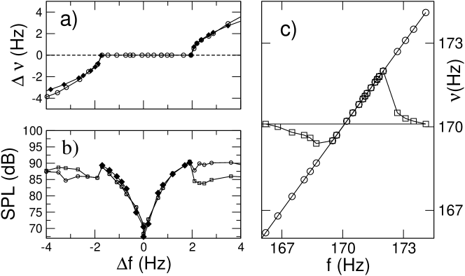
Figure 6: Frequency locking of two organ pipes. The plot shows the observed frequency difference $\Delta\nu$ versus the detuning of the uncoupled pipes, $\Delta f$ (circles). Upper left (a): In the synchronization region, a very clean plateau is observed. As in the case of external driving, the saddle-node bifurcation is observed at the edge to the synchronization region (filled diamonds). The agreement is very good. Lower left (b): Amplitudes at the first harmonics of the pipes (circles, variable-frequency pipe;squares, fixed-frequency pipe) against detuning; the sharp decrease of the amplitude at $\Delta f=0$ indicates an antiphase oscillation at the pipe mouth. The analytical curve obtained using synchronization theory is shown with filled diamonds, assuming $\phi_{0}=\pi$—the agreement is excellent. Right (c):Plot of the absolute frequencies (circles/squares as above),, the straight line shows the 170.1 Hz of the fixed-frequency pipe.

Varying the frequency mismatch $\Delta f$ we observe a gradual increase of the amplitude at the centerpoint, where the microphone is situated. In Fig. 6b, the result of the measurement is displayed: We see an excellent agreement of our estimate with the measurement. This behavior is observed as well in the spectral plot, Fig. 7. where one can observe the collapse of all sidebands in the measured spectrum to one single frequency as a very sharp transition.

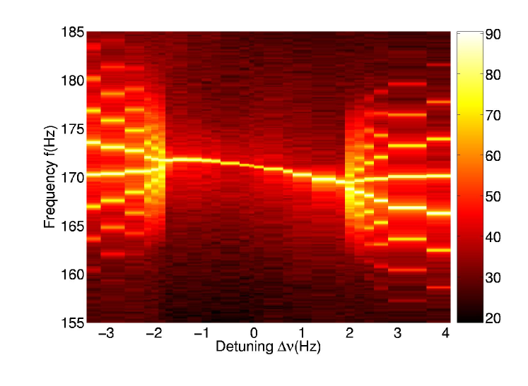
Figure 7: A sharp transition to synchronization is observed and the sidebands from beating in the measured spectrum collapse to a single frequency in the synchronization region. The amplitude is encoded according to the levels on the right.

For higher harmonics, the phase difference by $\phi_{0}$ does not imply destructive interference because they are slaved and follow the first harmonic. In other words, the relative phase for the $n$th harmonic in the synchronization region lies in the interval ($n(\phi_{0}-\pi/2),n(\phi_{0}+\pi/2)$). For the second harmonic, this implies in-phase oscillations at $\Delta f=0$. This is heard acoustically by a dominance of the octave around $\Delta f=0$. At the edge of the synchronization region, however, there is a phase difference of $\pi$ and destructive interference is expected. This is confirmed well by the quantitative measurement of the amplitude dependence of the second harmonic, shown in Fig. 8. The agreement with the estimate from superposition of two monopoles is still good, but deviations occur. Higher harmonics are in qualitative accordance with the above ideas, but quantitatively more and more differences are observed. This can be expected, because the approximation by a monopole source does not hold.

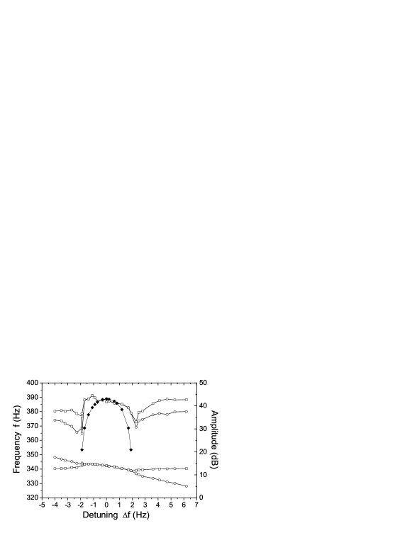
Figure 8: Amplitude and frequency difference for the second harmonic. Here, the phase is doubled and an annihilation occurs right at the edge of the synchronization region, seen as a sharp decrease. The curve predicted by theory shows deviations for the second harmonic.

When two pipes are coupled diffusively, a so-called oscillation death can occur, leading to a complete silence of both pipes. The whole input power would then be converted to heat without radiation. We thus observe a strong impact of the synchronization of the pipes on the acoustic properties of the emitted sound. From our results, we can rule out an oscillation death for two coupled pipes with zero detuning, as suggested in Pikovsky-Rosenblum-Kurths-01 . Rather, the two oscillators radiate two antiphase waves; this results in a vanishing acoustic signal.

D The Coupling of the Pipes

As in the case of the external driving by a loudspeaker, the two pipes interact by the pressure perturbation generated at the pipes mouths. But now, there are two sources of pressure contributions: the acoustic and the aerodynamic part from the vortices itself. Which one is dominant depends on the ratio of their amplitudes. In the case of the organ pipes, the acoustic pressure is very large due to the selected amplification of the resonator frequencies. However, the wind field at one pipe can literally “blow away” an adjacent vortex. On the basis of our observations, we can only state that definitely, the acoustical field is sufficient to give raise of synchronization. The influence of the wind field must be subject of careful future work including flow visualization on the scale of several vortex diameters. At the edge of the synchronization region, there must be a phase difference of $\phi_{0}\pm\pi/2$, which corresponds to a shift of a quarter of a jet oscillation. The jets then undergo a mutual reordering into a complex spatio-temporal three dimensional pattern. Again, the observation of the pattern was beyond the facilities of the current experimental setup.

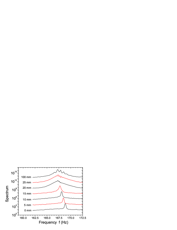
Figure 9: Frequency spectrum of the coupled pipes in dependence on the distance, given in the legend. The pipes decouple more and more when farther apart. For small distances, a sharp peak at the synchronization frequency is observed, for large distances, the peak broadens more and more, at very large distances the spectrum of the uncoupled pipes is recovered with the typical beat phenomenon. To distinguish different graphs, an offset has been added to each curve.

All our observations are consistent with an interpretation in the frame of synchronization theory of two oscillators. A full description of the physics has to take into account the origin of the sound generation—the oscillations of resonator and the vortices generated by two jets. Most likely, there is a competition of the interaction between jets and resonators. Which mechanism wins depends then on the ratio of the respective amplitudes. A comment should be made on why the synchronization description by two oscillators holds so well. In the measured Reynolds number regime, there might be three-dimensional patterns at the pipe mouth, if the aspect ratio is large enough. To check this in our particular case requires detailed experiments. Neglecting three dimensional structures, and assuming that the air sheet is homogeneously oscillating, a description by oscillator models like Stuart-Landau or a van-der-Pol equation could be sufficient to describe the two dimensional oscillations and the transition to turbulence Provansal-87 . Since the main sound production is due to the interaction with the labium, an oscillator model suits well. From synchronization theory it follows that any self-sustained oscillators will generically follow the synchronization scenario when coupled, leading to the observed behavior Pikovsky-Rosenblum-Kurths-01 ; Aronson-Ermentrout-Koppel-90 . The simulations in Stanzial-00 are completely in agreement with this fact. We are convinced that full understanding may be achieved by studying the details of the coupling mechanism.

To investigate the sensitivity to coupling strength, we measured the frequency spectrum about the first harmonic while varying inter-pipe distance (measured between the outer walls of the pipes). The detuning was fixed to 0.7 Hz. The corresponding plot is depicted in Fig. 9. For large distances, the typical interference pattern of two noninteracting oscillators is observed. As the pipes come closer to each other, the individual, sharp peaks of half width $\simeq$ 0.1 Hz reduce in amplitude and at the same time the spectrum broadens to a “hump” with half width $\simeq 1$ Hz. Peaks typical of the beating from linear superposition sit on the hump. Coming even closer, full synchronization is observed with one single, very sharp peak of again half width $\simeq 0.1$ Hz. That means the hump is about ten times broader than either of the peaks for the uncoupled system or the synchronized one.

The basic observations can be explained by synchronization theory. In Eq. 9, the square root behavior of the frequency difference at the transition to synchronization (the bifurcation point) is derived. Lowering the coupling strength is equivalent to shift the bifurcation point towards zero. At a certain distance the detuning leaves the synchronization region and one should observe a (strongly nonlinear) beat. The peaks of the beat are observable as small side peaks on top of the broad peak. For a pure beat, only sharp peaks should be observed. Here, the duration of the large time interval -we do not want to call it period- varies slightly such that the sidebands wiggle a bit, altogether this leads to a broad peak. To illustrate this behavior, we plot in Fig. 10 three different time signals for the distances 10 mm (synchronized), 15 mm (shortly before synchronization), and 25 mm. The fast oscillations look very similar for all of the distances, as exemplary given by Fig. 10 (bottom, right).

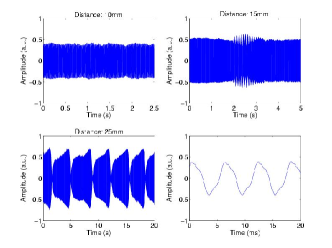
Figure 10: Time signal for three different distances. Upper left: 10mm, lower left: 15 mm, upper right:25 mm. The lower right graph shows a typical fast oscillation as found for all three distances. The transition from synchronization to beat happens between 15 and 25 mm. For 10 mm the amplitude is constant and the phase rotates with the fast frequency. At 25 mm the beat phenomenon is observed with a constant amplitude over relatively long times (e.g. ) and a quick phase slip (). At 15 mm, the system shows some intermittent bursts at irregular times.

A complete understanding why such a broad hump appears could not be achieved. There are several possible explanations. According to classical synchronization theory the frequency fluctuation cannot be explained but by noise, e.g. in the air supply in the wind system. Another option are the small fluctuations in the vortices at the pipe mouth which can be sufficient to cause the very small variation in the beat frequency. Finally, one can consider the bifurcation to synchronization as a kind of phase transition, where typically large fluctuations occur, including chaotic behavior. By means of our measurement we cannot decide which of these scenarios is true. Finally, we want to mention recent results concerning whistling of two nearby Helmholtz resonators show a similar transition in the phase of the acoustical signals emitted by the resonators Derks-Hirschberg-04 . Interestingly, the phase relation is lost at distances of the order of the ones we find (25mm, if the wall thickness of the pipes is included). Thus, this observation might be explained by synchronization as well.

IV Conclusion

We presented measurements on an external driving of an organ pipe by a loudspeaker and on the mutual influence of two organ pipes. The observed behavior is completely consistent with an explanation in the frame of synchronization theory. For the dependence of the synchronization on the “coupling strength”, measurements determining the dependence of the frequencies on the inter-pipe distance have been carried out. They reveal a broadening of the peak at the synchronization frequency with increasing distance. This broadening can be explained by quick phase slips as predicted by theory close to a saddle-node bifurcation. The smearing out of the side peaks of this beat can be either due to inconstant wind supply or due to the fluctuations caused by the oscillating air sheet at the pipe mouth. To clear this question further measurements have to be carried out.

From an acoustic point of view, one can address the question of how to position two organ pipes close in frequency. This has been intuitively solved by organ builders by trial and error in the last centuries Angster-93 . Our work might give quantitative hints on how large the inter-pipe distance needs to be to suppress mutual influence, and on details of the coupling mechanism. For example, avoiding an amplitude minimum for the first harmonic is highly desirable.

From an aerodynamical point of view, the above scenario requires more detailed investigations to understand the full dynamics of the coupled resonator/jet system, although a model consisting of two mutually coupled oscillators seems to be sufficient for all qualitative questions. In addition the more involved setup of more than two organ pipes is an interesting subject for further investigations. From our measurements, one can clearly say that the pipes do not show an oscillation death; rather, antiphase sound radiation yields the observed weakening of the amplitude.

References

- (1) B. Fabre and A. Hirschberg. Physical modeling of flue instruments: A review of lumped models. Acustica - Acta Acustica, 86:599–610, 2000.
- (2) N. H. Fletcher and T. D. Rossing. The physics of musical instruments. Springer, New York, 1998.
- (3) L. Cremer and H. Ising. Die selbsterregten Schwingungen von Pfeifen. Acustica, 19:143–153, 1967.
- (4) John W. Coltman. Sounding mechanism of the flute and organ pipe. J. Acoust. Soc. Am., 44(4):983–992, 1968.
- (5) John W. Coltman. Jet behavior in the flute. J. Acoust. Soc. Am., 92(1):74–83, July 1992.
- (6) N. H. Fletcher. Autonomous vibration of simple pressure-controlled valves in gas flows. J. Acoust. Soc. Am, 93:2172–2180, 1993.
- (7) A.W. Nolle. Flue organ pipes: Adjustments affecting steady waveform. J. Acoust. Soc. Am., 73(5):1821–1832, May 1983.
- (8) J. W. Coltman. Jet drive mechanisms in edge tones and organ pipes. J. Acoust. Soc. Am., 60(3):725–733, September 1976.
- (9) M. P. Verge, B. Fabre, W. E. A. Mahu, A. Hirschberg, R.R. van Hassel, A.P.J. Wijnands, J.J. de Vries, and C.J. Hogendoorn. Jet formation and jet velocity fluctuations in a flue organ pipe. J. Acoust. Soc. Am., 95(2):1119–1132, February 1994.
- (10) M. P. Verge, B. Fabre, A. Hirschberg, and A.P.J. Wijnands. Sound production in recorderlike instruments. i. dimensionless amplitude of the internal acoustic field. J. Acoust. Soc. Am., 101(5):2914–2924, May 1997.
- (11) M. P. Verge, A. Hirschberg, and R. Caussé. Sound production in recorderlike instruments. i. a simulation model. J. Acoust. Soc. Am., 101(5):2925–2939, May 1997.
- (12) B. Fabre, A. Hirschberg, and A. P. J. Wijnands. Vortex shedding in steady oscillation of a flue organ pipe. Acustica - Acta Acustica, 82:863–877, 1996.
- (13) C. Segoufin, B. Fabre, and L. de Lacombe. Experimental investigation of the flue channel geometry influence on edge-tone oscillations. Acta Acoustica united with Acustica, 90:966–975, 2004.
- (14) J. W. S. Rayleigh. The Theory of Sound, volume 2. Dover Publications, 1945.
- (15) H. Bouasse. Instruments a vent. Lib. Delagrave, Paris, 1929.
- (16) D. Stanzial, D. Bonsi, and D. Gonzales. Nonlinear modelling of the mitnahme-effekt in coupled organ pipes. In International symposium on musical acoustics (ISMA) 2001, Perugia, Italy, pages 333–337, 2001.
- (17) Judith Angster, József Angster, and András Miklós. Coupling between simultaneously sounded organ pipes. AES Preprint 94th Convention Berlin 1993, March 1993.
- (18) D. Zscherpel. Alexander Schuke GmbH, 2004. priv. comm.
- (19) A. Pikovsky, M. Rosenblum, and J. Kurths. Synchronization: A Universal Concept in Nonlinear Sciences. Cambridge University Press, Cambridge, Mass., 2001.
- (20) J. W. S. Rayleigh. On the pitch of organ-pipes. Phil. Mag., XIII:340–347, 1882.
- (21) Stefan Pitsch, Judith Angster, M. Strunz, and András Miklós. Spectral properties of the edge tone of a flue organ pipe. Proceed. International Symposium on Musical Acoustics, 1997, Edinburgh, 19(5):339–344, 1997.
- (22) N. H. Fletcher. Air flow and sound generation in musical wind instruments. Annual Review of Fluid Mechanics, 11:123–146, 1979.
- (23) N. H. Fletcher. The nonlinear physics of musical instruments. Rep. Prog. Phys., 62:723–764, 1999.
- (24) N. H. Fletcher. Mode locking in nonlinearly excited inharmonic musical oscillators. J. Acoust. Soc. Am., 64:1566–1569, 1978.
- (25) N. H. Fletcher. Sound production by organ flue pipes. J. Acoust. Soc. Am., 60(4):926–936, October 1976.
- (26) T. A. Johansson and M. Kleiner. Theory and experiments on the coupling of two helmholtz resonators. J. Acoust. Soc. Am., 110:1315–1328, 2001.
- (27) M. S. Howe. Contribution to the theory of aerodynamic sound, with application to excess jet noise and theory of the flute. J. Fluid Mech., 71:625–673, 1975.
- (28) M. S. Howe. Theory of vortex sound. Cambridge texts in applied mathematics. Cambridge University Press, Cambridge, UK, 2003.
- (29) M. S. Howe. Acoustics of fluid-structure interactions. Cambridge University Press, Cambridge, UK, 1998.
- (30) S. K. Lele. Computational aeroacoustics, a review. In Proc. 35th Aerospace Sciences Meeting and Exhibit, Reno, Nevada, 1997. AIAA Paper 97-0018.
- (31) C. K. W. Tam. Advances in numerical boundary conditions for computational aeroacoustics. J. Comp. Acoust., 6(4):377–402, 1998.
- (32) N. N. Bogoliubov and V. A. Mitropolsky. Asymptotic methods in the theory of non-linear oscillations. International Monographs on Advanced Mathematics and Physics, Gordon and Breach Science Publishers, New York, 1961. Translation from russian original (1955).
- (33) P. S. Landa. Nonlinear Oscillations and waves in dynamical systems. Kluwer Academic, Dordrecht, 1996.
- (34) R. Adler. A study of locking phenomena in oscillators. Proc. IRE, 34:351–357, 1946.
- (35) E. Ott, T. Sauer, and J.A. Yorke. Coping with Chaos. Series in Nonlinear Science. Wiley, New York, 1994.
- (36) M. Provansal, C. Mathis, and L. Boyer. Bénard-von Karman instability: transient and forced regimes. J. Fluid Mech., 182:1, 1987.
- (37) D. G. Aronson, G. B. Ermentrout, and N. Koppel. Amplitude response of coupled oscillators. Physica D, 41:403–449, 1990.
- (38) M. M. G. Derks and A. Hirschberg. Self-sustained oscillation of the flow along helmholtz resonators in a tandem configuration. In 8th International Conference on Flow Induced Vibration, FIV, pages 435–440, July 2004.