Statistical analysis of 22 public transport networks in Poland

Abstract

Public transport systems in 22 Polish cities have been analyzed. Sizes of these networks range from $N=152$ to $N=2881$. Depending on the assumed definition of network topology the degree distribution can follow a power law or can be described by an exponential function. Distributions of path lengths in all considered networks are given by asymmetric, unimodal functions. Clustering, assortativity and betweenness are studied. All considered networks exhibit small world behavior and are hierarchically organized. A transition between dissortative small networks $N\lesssim 500$ and assortative large networks $N\gtrsim 500$ is observed.

I Introduction

Since the explosion of the complex network science that has taken place after works of Watts and Strogatz watts_nat as well as Barabási and Albert barabasi_sci ; bamf a lot of real-world networks have been examined. The examples are technological networks (Internet, phone calls network), biological systems (food webs, metabolic systems) or social networks (co-authorship, citation networks) barabasi_rmp ; newman_siam ; mendes_book ; satorras_book . Despite this, at the beginning little attention has been paid to transportation networks - mediums as much important and also sharing as much complex structure as those previously listed. However, during the last few years several public transport systems (PTS) have been investigated using various concepts of statistical physics of complex networks amaral_pnas ; strogatz_nat ; albert_pre ; crucitti_physa ; marichiori_physa ; latora_prl ; latora_physa ; sen_pre ; seaton_physa ; guimera_arxiv ; guimera_epjb ; barrat_pnas ; li_pre ; bagler_arxiv .

Chronogically the first works regarding transportation networks have dealt with power grids barabasi_sci ; amaral_pnas ; watts_nat ; strogatz_nat . One can argue that transformators and transmission lines have little in common with PTS (i.e. underground, buses and tramways), but they definitely share at least one common feature: embedding in a two-dimensional space. Research done on the electrical grid in United States - for Southern California barabasi_sci ; amaral_pnas ; watts_nat ; strogatz_nat and for the whole country albert_pre as well as on the GRTN Italian power network crucitti_physa revealed a single-scale degree distributions ($p(k)\propto\exp(-\alpha k)$ with $\alpha\approx 0.5$), a small average connectivity values and relatively large average path lengths.

All railway and underground systems appear to share well known small-world properties watts_nat . Moreover this kind of networks possesses several other characteristic features. In fact Latora and Marichiori have studied in details a network formed by the Boston subway marichiori_physa ; latora_prl ; latora_physa . They have calculated a network efficiency defined as a mean value of inverse distances between network nodes. Although the global efficiency is quite large $E_{glob}=0.63$ the local efficiency calculated in the subgraphs of neighbors is low $E_{local}=0.03$ what indicates a large vulnerability of this network against accidental damages. However, the last parameter increases to $E_{local}^{{}^{\prime}}=0.46$ if the subway network is extended by the existing bus routes network. Taking into account geographical distances between different metro stations one can consider the network as a weighted graph and one is able to introduce a measure of a network cost. The estimated relative cost of the Boston subway is around 0.2 % of the total cost of fully connected network.

Sen et al. sen_pre have introduced a new topology describing the system as a set of train lines, not stops, and they have discovered a clear exponential degree distribution in Indian railway network. This system has shown a small negative value of assortativity coefficient. Seaton and Hackett seaton_physa have compared real data from underground systems of Boston (first presented in latora_physa ) and Vienna with the prediction of bipartite graph theory (here: graph of lines and graph of stops) using generation function formalism. They have found a good correspondence regarding value of average degree, however other properties like clustering coefficient or network size have shown differences of 30 to 50 percent.

In works of Amaral, Barrat, Guimerà et al. amaral_pnas ; guimera_arxiv ; guimera_epjb ; barrat_pnas a survey on the World-Wide Airport Network has been presented. The authors have proposed truncated power-law cumulative degree distribution $P(k)\propto k^{-\alpha}f(k/k_{x})$ with the exponent $\alpha=1.0$ and a model of preferential attachment where a new node (flight) is introduced with a probability given by a power-law or an exponential function of physical distance between connected nodes. However, only an introduction of geo-political constrains barrat_pnas (i.e. only large cities are allowed to establish international connections) explained the behavior of betweenness as a function of node degree.

Other works on airport networks in India li_pre and China bagler_arxiv have stressed small-world properties of those systems, characterized by small average path lengths ($\langle l\rangle\approx 2$) and large clustering coefficients ($c>0.6$) with comparison to random graph values. Degree distributions have followed either a power-law (India) or a truncated power-law (China). In both cases an evidence of strong disassortative degree-degree correlation has been discovered and it also appears that Airport Network of India has a hierarchical structure expressed by a power-law decay of clustering coefficient with an exponent equal to $1$.

In the present paper we have studied a part of data for PTS in $22$ Polish cities and we have analyzed their nodes degrees, path lengths, clustering coefficients, assortativity and betweenness. Despite large differences in sizes of considered networks (number of nodes ranges from $N=152$ to $N=2881$) they share several universal features such as degree and path length distributions, logarithmic dependence of distances on nodes degrees or a power law decay of clustering coefficients for large nodes degrees. As far as we know, our results are the first comparative survey of several public transport systems in the same country using universal tools of complex networks.

II The idea of space L and P

To analyze various properties of PTS one should start with a definition of a proper network topology. The idea of the space L and P, proposed in a general form in sen_pre and used also in seaton_physa is presented at Fig. 1. The first topology (space L) consists of nodes representing bus, tramway or underground stops and a link between two nodes exists if they are consecutive stops on the route. The node degree $k$ in this topology is just the number of directions (it is usually twice the number of all PTS routes) one can take from a given node while the distance $l$ equals to the total number of stops on the path from one node to another.

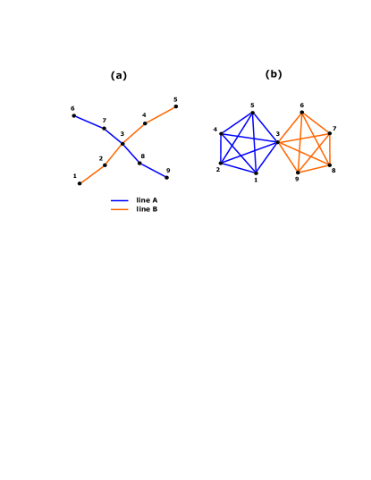
Figure 1: (Color online) Explanation of the space L (a) and the space P (b).

Although nodes in the space P are the same as in the previous topology, here an edge between two nodes means that there is a direct bus, tramay or underground route that links them. In other words, if a route $A$ consists of nodes $a_{i}$, i.e. $A={\{a_{1},a_{2},...,a_{n}\}}$, then in the space P the nearest neighbors of the node $a_{1}$ are $a_{2},a_{3},...,a_{n}$. Consequently the node degree $k$ in this topology is the total number of nodes reachable using a single route and the distance can be interpreted as a number of transfers (plus one) one has to take to get from one stop to another.

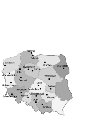
Figure 2: Map of examined cities in Poland.

Another idea of mapping a structure embedded in two-dimensional space into another, dimensionless topology has recently been used by Rosvall et al. in rosvall_prl where a plan of the city roads has been mapped into an ”information city network”. In the last topology a road represents a node and an intersection between roads - an edge, so the network shows information handling that has to be performed to get oriented in the city.

We need to stress that the spaces L and P do not take into account Euclidean distance between nodes. Such an approach is similar to the one used for description of several other types of network systems: Internet barabasi_sci , power grids albert_pre ; crucitti_physa , railway sen_pre or airport networks li_pre ; bagler_arxiv .

III Explored systems

	basic parameters			space L				space P
city	N	S	I	$\langle l\rangle_{L}$	$\langle k\rangle_{L}$	$c_{L}$	$r_{L}$	$\langle l\rangle_{P}$	$\langle k\rangle_{P}$	$c_{P}$	$r_{P}$
Piła	152	103	77	7.86	2.90	0.143	0.236	1.82	38.68	0.770	0.022
Bełchatów	174	35	65	16.94	2.62	0.126	0.403	1.71	49.92	0.847	-0.204
Jelenia Góra	194	109	93	11.14	2.53	0.109	0.384	2.01	32.94	0.840	0.000
Opole	205	96	129	10.29	3.03	0.161	0.320	1.80	50.19	0.793	-0.108
Toruń	243	116	206	10.24	2.72	0.134	0.068	2.12	35.84	0.780	-0.055
Olsztyn	268	88	173	12.02	3.08	0.111	0.356	1.91	52.91	0.724	0.020
Gorzów Wlkp.	269	77	162	16.41	2.48	0.082	0.401	2.40	38.51	0.816	-0.033
Bydgoszcz	276	174	386	10.48	2.61	0.094	0.147	2.10	33.13	0.799	-0.068
Radom	282	112	232	10.97	2.84	0.089	0.348	1.98	48.14	0.786	-0.067
Zielona Góra	312	58	119	6.83	2.97	0.067	0.237	1.97	44.77	0.741	-0.115
Gdynia	406	136	255	11.41	2.78	0.153	0.307	2.22	52.68	0.772	-0.018
Kielce	414	109	93	16.98	2.68	0.122	0.396	2.05	48.15	0.771	-0.106
Czȩstochowa	419	160	256	16.82	2.55	0.055	0.220	2.11	57.44	0.776	-0.126
Szczecin	467	301	417	12.34	2.54	0.059	0.042	2.47	34.55	0.794	-0.004
Gdańsk	493	262	458	16.14	2.61	0.132	0.132	2.30	40.52	0.804	-0.058
Wrocław	526	293	637	12.52	2.78	0.147	0.286	2.24	50.83	0.738	0.048
Poznań	532	261	577	14.94	2.72	0.136	0.194	2.47	44.87	0.760	0.160
Białystok	559	90	285	11.93	2.76	0.032	0.004	2.00	62.55	0.682	-0.076
Kraków	940	327	738	21.52	2.52	0.106	0.266	2.71	47.53	0.779	0.212
Łódź	1023	294	800	17.10	2.83	0.065	0.070	2.45	59.79	0.721	0.073
Warszawa	1530	494	1615	19.62	2.88	0.149	0.340	2.42	90.93	0.691	0.093
GOP	2811	1412	2100	19.76	2.83	0.085	0.208	2.90	68.42	0.760	-0.039

Table 1: Data gathered on 22 cities in Poland. $S$ stands for the surface occupied by the city (in $km^{2}$) note1 , $I$ is the city’s population in thousands of inhabitants note1 and $N$ is the number of nodes (stops) in the network. $\langle l\rangle$ is the average path length, $\langle k\rangle$ - the average degree value, $c$ is the clustering coefficient and $r$ - the assortativity coefficient. Indexes $L$ and $P$ stand, consequently, for the space L and the space P. Properties of parameters defined in spaces L and P will be discussed in sec. IV-VII

We have analyzed PTS (bus and tramways systems) in $22$ Polish cities, located in various state districts as it is depicted at Fig. 2. Table 1 gathers fundamental parameters of considered cities and data on average path lengths, average degrees, clustering coefficients as well as assortativity coefficients for corresponding networks.

Numbers of nodes in different networks (i.e. in different cities) range from $N=152$ to $N=2811$ and they are roughly proportional to populations $I$ and surfaces $S$ of corresponding cities (see Fig. 3). One should notice that other surveys exploring the properties of transportation networks have usually dealt with smaller numbers of vertices, such as $N=76$ for U-Bahn network in Vienna seaton_physa , $N=79$ for Airport Network of India (ANI) bagler_arxiv , $N=124$ in Boston Underground Transportation System (MBTA) latora_physa or $N=128$ in Airport Network of China (ANC) li_pre . Only in the case of the Indian Railway Network (IRN) sen_pre where $N=579$ and World-Wide Airport Network (WAN) barrat_pnas with $3880$ nodes sizes of networks have been similar or larger than for PTS in Poland. Very recently, von Ferber et al. ferber_cmp have presented a paper on three large PTS: Düsseldorf with $N=1615$, Berlin with $N=2952$ and Paris where $N=4003$.

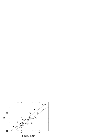
Figure 3: Log-log plot of the dependence of number of nodes $N$ on surface $S$ (circles) and population $I$ (triangles).

IV Degree distributions

IV.1 Degree distribution in the space L

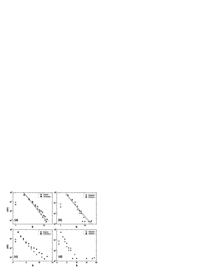
Figure 4: Degree distributions in the space L for four chosen cities. Plots (a) and (b) show the distributions in log-log scale while plots (c) and (d) - in the semi-log scale.

Fig. 4 shows typical plots for degree distribution in the space L. One can see that there is a slightly better fit to the linear behavior in the log-log description as compared to semi-logarithmic plots. Points $k=1$ are very peculiar since they correspond to routes’ ends. Remaining parts of degree distributions can be approximately described by a power law

$$p(k)\sim k^{-\gamma}$$ (1)

although the scaling cannot be seen very clearly and it is limited to less than one decade. Pearson correlation coefficients of the fit to Eq. (1) range from 0.95 to 0.99. Observed characteristic exponents $\gamma$ are between $2.4$ and $4.1$ (see Table 2), with the majority (15 out of 22) $\gamma>3$. Values of exponents $\gamma$ are significantly different from the value $\gamma=3$ which is characteristic for Barabási-Albert model of evolving networks with preferential attachment bamf and one can suppose that a corresponding model for transport network evolution should include several other effects. In fact various models taking into account effects of fitness, atractiveness, accelerated growth and aging of vertices mendes_adv or deactivation of nodes vazquez_pre ; klemm_pre lead to $\gamma$ from a wide range of values $\gamma\in\langle 2,\infty)$. One should also notice that networks with a characteristic exponent $\gamma>4$ are considered topologically close to random graphs havlin_prl - the degree distribution is very narrow - and a difference between power-law and exponential behavior is very subtle (see the Southern California power grid distribution in barabasi_sci presented as a power-law with $\gamma\approx 4$ and in strogatz_nat depicted as a single-scale cumulative distribution).

Degree distributions obtained for airport networks are also power-law (ANC, ANI) or power-law with an exponential cutoff (in the case of WAN). For all those systems exponent $\gamma$ is in the range of $2.0-2.2$, which differs significantly from considered PTS in Poland, however one has to notice, that airport networks are much less dependent on the two-dimensional space as it is in the case of PTS. This effect is also seen when analyzing average connectivity ($\langle k\rangle=5.77$ for ANI, $\langle k\rangle=9.7$ for WAN and $\langle k\rangle=12-14$ for ANC depending on the day of the week the data have been collected).

Let us notice that the number of nodes of degree $k=1$ is smaller as compared to the number of nodes of degree $k=2$ since $k=1$ nodes are ends of transport routes. The maximal probability observed for nodes with degree $k=2$ means that a typical stop is directly connected to two other stops. Still some nodes (hubs) can have a relatively high degree value (in some cases above 10) but the number of such vertices is very small.

IV.2 Degree distribution in the space P

In our opinion, the key structure for the analysis of PTS are routes and not single bus/tramway stops. Therefore we especially take under consideration the degree distribution in the space P.

To smooth large fluctuations, we use here the cumulative distribution $P(k)$ newman_siam according to the formula

$$P(k)=\int^{k_{max}}_{k}p(k)dk$$ (2)

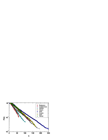
Figure 5: (Color online) $P(k)$ distribution in the space P for eight chosen cities

The cumulative distributions in the space P for eight chosen cities are shown at Fig 5. Using the semi-log scale we observe an exponential character of such distributions:

$$P(k)=Ae^{-\alpha k}$$ (3)

As it is well known bamf the exponential distribution (3) can occur for evolving networks when nodes are attached completely randomly. This suggests that a corresponding evolution of public transport in the space P possesses an accidental character that can appear because of large number of factors responsible for urban development. However in the next sections we show that other network’s parameters such as clustering coefficients or degree-degree correlations calculated for PTS are much larger as compared to corresponding values of randomly evolving networks analyzed in bamf .

In the case of IRN sen_pre degree distribution in the space P has also maintained the single-scale character $P(k)\sim e^{-\alpha k}$ with the characteristic exponent $\alpha=0.0085$. Values of average connectivity in the studies of MBTA ($\langle k\rangle=27.60$) and U-Bahn in Vienna ($\langle k\rangle=20.66$) are smaller than for considered systems in Poland, however one should notice that sizes of networks in MBTA and Vienna are also smaller.

city	$\gamma$	$\Delta\gamma$	$\alpha$	$\Delta\alpha$
Piła	2.86	0.17	0.0310	0.0006
Bełchatów	2.8	0.4	0.030	0.002
Jelenia Góra	3.0	0.3	0.038	0.001
Opole	2.29	0.23	0.0244	0.0004
Toruń	3.1	0.4	0.0331	0.0006
Olsztyn	2.95	0.21	0.0226	0.0004
Gorzów Wlkp.	3.6	0.3	0.0499	0.0009
Bydgoszcz	2.8	0.3	0.0384	0.0004
Radom	3.1	0.3	0.0219	0.0004
Zielona Góra	2.68	0.20	0.0286	0.0003
Gdynia	3.04	0.2	0.0207	0.0003
Kielce	3.00	0.15	0.0263	0.0004
Czȩstochowa	4.1	0.4	0.0264	0.0004
Szczecin	2.7	0.3	0.0459	0.0006
Gdańsk	3.0	0.3	0.0304	0.0006
Wrocław	3.1	0.4	0.0225	0.0002
Poznań	3.6	0.3	0.0276	0.0003
Białystok	3.0	0.4	0.0211	0.0002
Kraków	3.77	0.18	0.0202	0.0002
Łódź	3.9	0.3	0.0251	0.0001
Warszawa	3.44	0.22	0.0127	0.0001
GOP	3.46	0.15	0.0177	0.0002

Table 2: Coefficients $\gamma$ and $\alpha$ with their fitting errors $\Delta\gamma$ and $\Delta\alpha$. Fitting to the scaling relation (1) has been performed at whole ranges of degrees $k$ while fitting to (3) has been performed at approximately half of available ranges to exclude large fluctuations occurring for higher degrees (See Fig. 5).

IV.3 Average degree and average square degree

Taking into account the normalization condition $P(k_{min})=1$ we get the following equations for the average degree and the average square degree:

$$\langle k\rangle=\frac{k_{min}e^{-\alpha k_{min}}-k_{max}e^{-\alpha k_{max}}}{e^{-\alpha k_{min}}-e^{-\alpha k_{max}}}+\frac{1}{\alpha}$$ (4)

$$\langle k^{2}\rangle=\frac{k^{2}_{min}e^{-\alpha k_{min}}-k^{2}_{max}e^{-\alpha k_{max}}}{e^{-\alpha k_{min}}-e^{-\alpha k_{max}}}+{}$$ (5)

$${}+\frac{2(k_{min}e^{-\alpha k_{min}}-k_{max}e^{-\alpha k_{max}})}{\alpha(e^{-\alpha k_{min}}-e^{-\alpha k_{max}})}+\frac{2}{\alpha^{2}}$$

Dropping all terms proportional to $e^{-\alpha k_{max}}$ we receive simplified equations for $\langle k\rangle$ i $\langle k^{2}\rangle$:

$$\langle k\rangle\approx k_{min}+\frac{1}{\alpha}$$ (6)

$$\langle k^{2}\rangle\approx k^{2}_{min}+\frac{2k_{min}}{\alpha}+\frac{2}{\alpha^{2}}$$ (7)

Since values of $k_{min}$ range between $3$ and $16$ and they are independent from network sizes $N$ as well as observed exponents $\alpha$ we have approximated $k_{min}$ in Eqs. (6) - (7) by an average value (mean arithmetical value) for considered networks, $\langle k_{min}\rangle\approx 8.5$. At Figs. 6 and 7 we present a comparison between the real data and values calculated directly form Eqs. (6) and (7).

Figure 6: $\langle k\rangle$ as a function of $\alpha$. Circles are real data values, while the line corresponds to Eq. (6)

Figure 7: $\langle k^{2}\rangle$ as a function of $\alpha$. Circles are real data values, while the line corresponds to Eq. (7)

V Path length’s properties

V.1 Path length’s distributions

Plots presenting path length distributions $p(l)$ in spaces L and P are shown at Figs. 8 and 9 respectively. The data well fit to asymmetric, unimodal functions. In fact for all systems a fitting by Lavenberg - Marquardt method has been made using the following trial function:

$$p(l)=Ale^{-Bl^{2}+Cl}$$ (8)

where $A,B$ and $C$ are fitting coefficients.

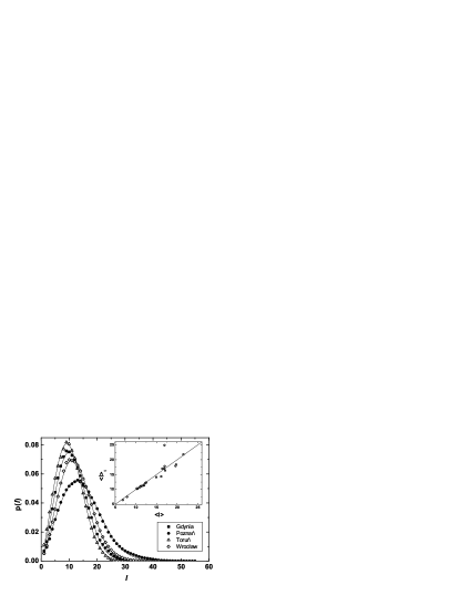
Figure 8: Fitted path length distribution in the space L

Inserts at Figs. 8 and 9 present a comparison between experimental results of $\langle l\rangle$ and corresponding mean values obtained from Eq. (8). One can observe a very good agreement between averages from Eq. (8) and experimental data.

The agreement is not surprising in the case of Fig. 9 since the number of fitted data points to curve (8) is quite small, but it is more prominent for Fig. 8.

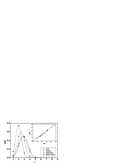
Figure 9: Fitted path length distribution in the space P.

Ranges of distances in the space L are much broader as compared to corresponding ranges in the space P what is a natural effect of topology differences. It follows that the average distance in the space P is much smaller ($\langle l\rangle<3$) than in the space L. The characteristic length 3 in the space P means that in order to travel between two different points one needs in average no more than two transfers. Other PTS also share this property, depending on the system size the following results have been obtained: $\langle l\rangle=1.81$ (MBTA), $\langle l\rangle=1.86$ (Vienna), $\langle l\rangle=2.16$ (IRN). In the case of the space L the network MBTA with its average shortest path length $\langle l\rangle=15.55$ is placing itself among the values acquired for PTS in Poland. Average path length in airport networks is very small: $\langle l\rangle=2.07$ for ANC, $\langle l\rangle=2.26$ for ANI and $\langle l\rangle=4.37$ for WAN. However, because flights are usually direct (i.e. there are no stops between two cities) one sees immediately that the idea of the space L does not apply to airport networks - they already have an intrinsic topology similar to the space P. Average shortest path lengths $\langle l\rangle$ in those systems should be relevant to values obtained for other networks after a transformation to the space P.

The shape of path length distribution can be explained in the following way: because transport networks tend to have an inhomogeneous structure, it is obvious that distances between nodes lying on the suburban routes are quite large and such a behavior gives the effect of observed long tails in the distribution. On the other hand shortest distances between stops not belonging to suburban routes are more random and they follow the Gaussian distribution. A combined distribution has an asymmetric shape with a long tail for large paths.

We need to stress that inter-node distances calculated in the space L are much smaller as compared to the number of network nodes (see Table I). Simultaneously clustering coefficients $c_{L}$ are in the range $\langle 0.03,0.15\rangle$. Such a behavior is typical for small-world networks watts_nat and the effect has been also observed in other transport networks amaral_pnas ; latora_physa ; sen_pre ; seaton_physa ; li_pre ; bagler_arxiv . The small world property is even more visible in the space P where average distances are between $\langle 1.80,2.90\rangle$ and the clustering coefficient $c_{P}$ ranges from 0.682 to 0.847 which is similar to MBTA ($c=0.93$), Vienna ($c=0.95$) or IRN ($c=0.69$).

V.2 Path length as function of product $k_{i}k_{j}$

In agatac an analytical estimation of average path length $\langle l\rangle$ in random graphs has been found. It has been shown that $\langle l\rangle$ can be expressed as a function of the degree distribution. In fact the mean value for shortest path length between $i$ and $j$ can be written as agatac :

$$l_{ij}(k_{i},k_{j})=\frac{-\ln k_{i}k_{j}+\ln\left(\langle k^{2}\rangle-\langle k\rangle\right)+\ln N-\gamma}{\ln\left(\langle k^{2}\rangle/\langle k\rangle-1\right)}+\frac{1}{2}$$ (9)

where $\gamma=0.5772$ is Euler constant.

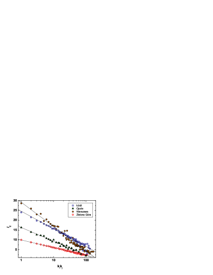
Figure 10: (Color online) Dependence of $l_{ij}$ on $k_{i}k_{j}$ in the space L

Since PTS are not random graphs and large degree-degree correlation in such networks exist we have assumed that Eq. (9) is only partially valid and we have written it a more general form nasz_physa ; nasz_prl ; nasz_aip ; nasz_app :

$$\langle l_{ij}\rangle=A-B\log k_{i}k_{j}.$$ (10)

To check the validity of Eq. (10) we have calculated values of average path length between $l_{ij}$ as a function of their degree product $k_{i}k_{j}$ for all systems in the space L . The results are shown at Fig. 10, which confirms the conjunction (10). A similar agreement has been received for the majority of investigated PTS. Eq. (10) can be justified using a simple model of random graphs and a generating function formalism motter or a branching tree approach nasz_physa ; nasz_prl ; nasz_aip ; nasz_app . In fact the scaling relation (10) can be also observed for several other real world networks nasz_physa ; nasz_prl ; nasz_aip ; nasz_app .

It is useless to examine the relation (10) in the space P because corresponding sets $l_{ij}$ consist usually of 3 points only.

VI Clustering coefficient

We have studied clustering coefficients $c_{i}$ defined as a probability that two randomly chosen neighbors of node $i$ possess a common link.

The clustering coefficient of the whole network seems to depend weakly on parameters of the space L and of the space P. In the first case its behavior with regard to network size can be treated as fluctuations, when in the second one it is possible to observe a small decrease of $c$ along with the networks size (see Table 1). We shall discuss only properties of the clustering coefficients in the space P since the data in the space L are meaningless.

It has been shown in sen_pre that clustering coefficient in IRN in the space P decays linearly with the logarithm of degree for large $k$ and is almost constant (and close to unity) for small $k$. In the considered PTS we have found that this dependency can be described by a power law (see Fig. 11):

$$c(k)\sim k^{-\beta}$$ (11)

Such a behavior has been observed in many real systems with hierarchical structures ravasz_pre ; ravasz_sci . In fact, one can expect that PTS should consist of densely connected modules linked by longer paths.

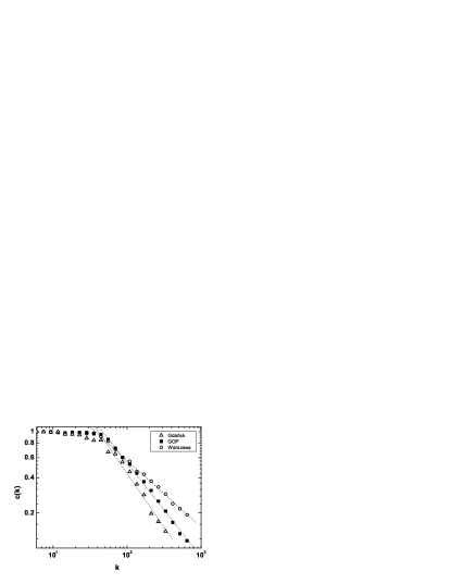
Figure 11: $c(k)$ for Gdańsk (triangles) GOP (squares) and Warszawa (circles). Dashed lines are fits to Eq. (11) with following exponents: Gdańsk - $\beta=0.93\pm 0.05$, GOP - $\beta=0.81\pm 0.02$ and Warszawa - $\beta=0.57\pm 0.01$. All data are logarithmically binned with the power of 1.25.

Observed values of exponents $\beta$ are in the range $\beta\in\langle 0.54,0.93\rangle$. This can be explained using a simple example of a star network: suppose that the city transport network is a star consisting of $n$ routes with $L$ stops each. Node $i$, at which all $n$ routes cross is a vertex that has the highest degree in the network. We do not allow any other crossings among those $n$ routes in the whole system. It follows that the degree of node $i$ is $k_{i}=n(L-1)$ and the total number of links among the nearest neighbors of $i$ is $E_{i}=n(L-1)(L-2)/2$. In other words the value of the clustering coefficient for the node with the maximum degree is:

$$c(k_{max})=\frac{2E_{i}}{k_{i}(k_{i}-1)}=\frac{L-2}{n(L-1)-1}$$ (12)

where $k_{max}=n(L-1)$. It is obvious that the minimal degree in the network is $k_{min}=L-1$ and this correspondences to the value $c(k_{min})=1$. Using these two points and assuming that we have a power-law behavior we can express $\beta$ as:

$$\beta=-\frac{\ln c(k_{max})-\ln c(k_{min})}{\ln k_{max}-\ln k_{min}}=-\frac{\ln\frac{L-2}{n(L-1)-1}}{\ln n}$$ (13)

Because $n(L-1)\gg 1$ and $L-1\approx L-2$ we have $\beta\approx 1$.

In real systems the value of clustering coefficient of the highest degree node is larger than in Eq. (12) due to multiple crossings of routes in the whole network what leads to a decrease of the exponent $\beta$ (see Fig. 11). This decrease is also connected to the presence of degree-degree correlations (see the next Section).

VII Degree-degree correlations

To analyze degree-degree correlations in PTS we have used the assortativity coefficient $r$, proposed by Newman new2 that corresponds to the Pearson correlation coefficient new4 of the nodes degrees at the end-points of link:

$$r=\frac{\sum_{i}j_{i}k_{i}-\frac{1}{M}\sum_{i}j_{i}\sum_{i}k_{i}}{\sqrt{\sum_{i}j_{i}^{2}-\frac{1}{M}(\sum_{i}j_{i})^{2}}\sqrt{\sum_{i}k_{i}^{2}-\frac{1}{M}(\sum_{i}k_{i})^{2}}}$$ (14)

where $M$ - number of pairs of nodes (twice the number of edges), $j_{i},k_{i}$ - degrees of vertices at both ends of $i$-th pair and index $i$ goes over all pairs of nodes in the network.

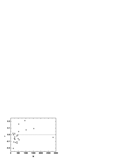
Figure 12: The assortativity coefficient $r$ in the space P as a function of $N$

Values of the assortativity coefficient $r$ in the space L are independent of the network size and are always positive (see Table 1), what can be explained in the following way: there is a little number of nodes characterized by high values of degrees $k$ and they are usually linked among themselves. The majority of remaining links connect nodes of degree $k=2$ or $k=1$, because $k=2$ is an overwhelming degree in networks.

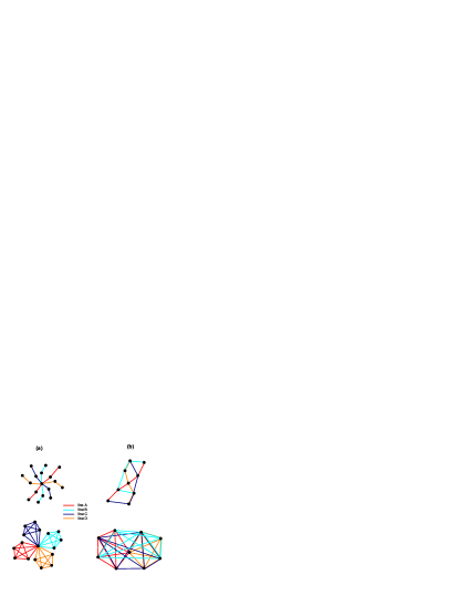
Figure 13: (Color online) Crossing of 4 routes of 5 stops each. (a) In the star example there is only one hub and assortativity coefficient is equal to $r=-0.25$ according to Eq. (15). In case (b) a few hubs exist due to a multiple crossing of routes and $r=-0.19$. Upper diagrams - the space L, lower diagrams - the space P.

Similar calculations performed for the space P lead to completely different results (Fig. 12). For small networks the correlation parameter $r$ is negative and it grows with $N$, becoming positive for $N\gtrsim 500$. The dependence can be explained as follows: small towns are described by star structures and there are only a few doubled routes, so in this space a lot of links between vertices of small and large $k$ exist. Using the previous example of a star network and taking into account that the degree of the central node is equal to $k_{c}=n(L-1)$, the degree of any other node is $k_{o}=L-1$, after some algebra we receive the following expression for the assortativity coefficient of such a star network:

$$r=-\frac{1}{L-1}$$ (15)

Let us notice that the coefficient $r$ is independent from the number of crossing routes and is always a negative number.

On the contrary, in the large cities there are lots of connections between nodes characterized by large $k$ (transport hubs) as well as there is a large number of routes crossing in more than one point (see Fig. 13). It follows that the coefficient $r$ can be positive for such networks. A strange behavior for the largest network (GOP) can be explained as an effect of its peculiar structure: the system is rather a conglomerate of many towns than a single city. Thus, the value of $r$ is lowered by single links between the subsets of this network.

At Fig. 14 we show coefficients $\beta$ as a function of $r$ in the space P. One can see that in general positive values of the assortativity coefficient correspond to lower values of $\beta$, being an effect of existence of several links between hubs in the networks.

Reported values of assortativity coefficients in other transport networks have been negative ($r=-0.402$ for ANI li_pre and $r=-0.033$ for IRN sen_pre ) and since these systems are of the size $N<600$ thus it is in agreement with our results.

Figure 14: $\beta$ coefficient (see Eq. (11)) as a function of the assortativity coefficient $r$ in the space P.

VIII Betweenness

The last property of PTS examined in this work is betweenness soc which is the quantity describing the ”importance” of a specific node according to equation bar1 :

$$g(i)=\sum_{j\neq k}\frac{\sigma_{jk}(i)}{\sigma_{jk}}$$ (16)

where, $\sigma_{jk}$ is a number of the shortest paths between nodes $j$ and $k$, while $\sigma_{jk}(i)$ is a number of these paths that go through the node $i$.

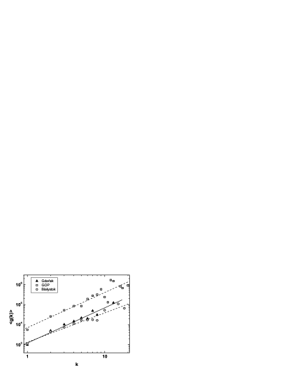
Figure 15: The average betweenness $\langle g\rangle$ as a function of $k$ in the space L for three chosen cities.

Figure 16: $\eta$ coefficient as a function of network size $N$

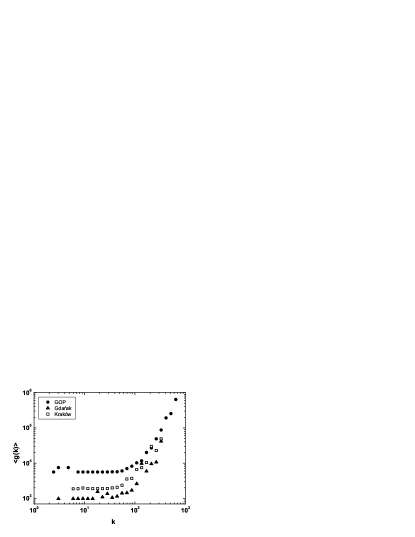
Figure 17: The average betweenness $\langle g\rangle$ as a function of $k$ in the space P for three chosen cities.

VIII.1 Betweenness in the space L

Fig. 15 shows dependence of the average betweenness $\langle g\rangle$ on node degree calculated using the algorithm proposed in new3 (see also brandes ). Data at Fig. 15 fit well to the scaling relation:

$$g\sim k^{\eta}$$ (17)

observed in Internet Autonomous Systems vaz , co-authorship networks goh and BA model or Erdős-Rényi random graphs bar1 .

The coefficient $\eta$ is plotted at Fig. 16 as a function of network size. One can see, that $\eta$ is getting closer to 2 for large networks. Since it has been shown that there is $\eta=2$ for random graphs bar1 with Poisson degree distribution thus it can suggest that large PTS are more random than small ones. Such an interpretation can be also received from the Table 2 where larger values of the exponent $\gamma$ are observed for large cities.

VIII.2 Betweenness in the space P

The betweenness as a function of node degree $k$ in the space P is shown at Fig. 17. One can see large differences between Fig. 15 and 17. In the space P there is a saturation of $\langle g\rangle$ for small $k$ what is a result of existence of the suburban routes while the scale-free behavior occurs only for larger $k$. The saturation value observed in the limit of small $k$ is given by $\langle g(k_{min})\rangle=2(N-1)$ and the length of the saturation line increases with the mean value of a single route’s length observed in a city.

IX Conclusions

In this study we have collected and analyzed data for public transport networks in 22 cities that make over 25 % of population in Poland. Sizes of these networks range from $N=152$ to $N=2881$. Using the concept of different network topologies we show that in the space L, where distances are measured in numbers of passed bus/tramway stops, the degree distributions are approximately given by a power laws with $\gamma=2.4-4.1$ while in the space P, where distances are measured in numbers of transfers, the degree distribution is exponential with characteristic exponents $\alpha=0.013-0.050$. Distributions of paths in both topologies are approximately given by a function $p(l)=Ale^{-Bl^{2}+Cl}$. Small world behavior is observed in both topologies but it is much more pronounced in space P where the hierarchical structure of network is also deduced from the behavior of $c(k)$. The assortativity coefficient measured in the space L remains positive for the whole range of $N$ while in the space P it changes from negative values for small networks to positive values for large systems. In the space L distances between two stops are linear functions of the logarithm of their degree products.

Many of our results are similar to features observed in other works regarding transportation networks: underground, railway or airline systems amaral_pnas ; marichiori_physa ; latora_prl ; latora_physa ; sen_pre ; seaton_physa ; guimera_arxiv ; guimera_epjb ; barrat_pnas ; li_pre ; bagler_arxiv ; ferber_cmp . All such networks tend to share small-world properties and show strong degree-degree correlations that reveal complex nature of those structures.

- (1) D. J. Watts and S. H. Strogatz, Nature 393, 440 (1998).
- (2) A.-L. Barabási and R. Albert, Science 286, 509 (1999).
- (3) A.-L. Barabási, R. Albert and H. Joeng, Physica A 272, 173 (1999).
- (4) R. Albert and A.-L. Barabási, Rev. Mod. Phys. 74 47 (2002).
- (5) M. E. J. Newman, SIAM Rev. 45, 167 (2003).
- (6) J. F. F. Mendes, S. N. Dorogovtsev and A. F. Ioffe, Evolution of networks: From Biological Nets to the Interent and WWW (Oxford University Press, Oxford, 2003).
- (7) R. Pastor-Satorras and A. Vespignani, Evolution and Structure of the Internet: A Statistical Physics Approach (Cambridge University Press, Cambridge, 2004).
- (8) L. A. N. Amaral, A. Scala, M. Barthèlèmy and H.E. Stanley, Proc. Nat. Acad. Sci. USA 97 11149 (2000).
- (9) S. H. Strogatz, Nature 410, 268 (2001).
- (10) R. Albert, I. Albert and G. L. Nakarado Phys. Rev. E 69, 025103(R) (2004).
- (11) P. Crucitti, V. Latora, M. Marchiori, Physica A 338, 92 (2004).
- (12) M. Marchiori, V. Latora, Physica A 285, 539 (2000).
- (13) V. Latora and M. Marchiori, Phys. Rev. Lett. 87, 198701 (2001).
- (14) V. Latora, M. Marchiori, Physica A 314, 109 (2002).
- (15) P. Sen, S. Dasgupta, A. Chatterjee, P. A. Sreeram, G. Mukherjee and S. S. Manna, Phys. Rev. E 67, 036106 (2003).
- (16) K. A. Seaton and L. M. Hackett, Physica A 339, 635 (2004).
- (17) R. Guimerà, S. Mossa, A. Turtschi and L. A. N. Amaral, arXiv:cond-mat/0312535 (2003).
- (18) R. Guimerà and L. A. N. Amaral, Eur. Phys. J. B 38, 381 (2004).
- (19) A. Barrat, M. Barthèlèmy, R. Pastor-Satorras, and A. Vespignani, Proc. Natl. Acad. Sci. USA 101, 3747 (2004).
- (20) W. Li and X. Cai, Phys. Rev. E 69, 046106 (2004).
- (21) G. Bagler, arXiv:cond-mat/0409773 (2004).
- (22) M. Rosvall, A. Trusina, P. Minnhagen, and K. Sneppen, Phys. Rev. Let. 94, 028701 (2005).
- (23) C. von Ferber, Yu. Holovatch, and V. Palchykov, Condens. Matt. Phys. 8, 225 (2005).
- (24) Data on population and city surfaces have been taken form the official site of the Polish national Central Statistical Office (http://www.stat.gov.pl/bdrpuban/ambdr.html). One should mention here that S and I for GOP (Upper-Silesian Industry Area) are the sum of the values for several towns GOP consits of.
- (25) L. A. Braunstein, S. V. Buldyrev, R. Cohen, S. Havlin and H. E. Stanley, Phys. Rev. Lett. 91, 168701 (2003).
- (26) S. N. Dorogovtsev and J. F. F. Mendes, Advances in Physics 51, 4, 1079 (2002).
- (27) A. Vázquez, M. Boguñá, Y. Moreno, R. Pastor-Satorras, and A. Vespignani, Phys. Rev. E 67, 046111 (2003).
- (28) K. Klemm and V. M. Eguíluz, Phys. Rev. E 65, 036123 (2002).
- (29) A. Fronczak, P. Fronczak and J.A. Hołyst, Phys. Rev. E 68, 046126 (2003).
- (30) J.A. Hołyst, J. Sienkiewicz, A. Fronczak, P. Fronczak, and K. Suchecki, Physica A 351, 167 (2005).
- (31) J.A. Hołyst, J. Sienkiewicz, A. Fronczak, P. Fronczak, and K. Suchecki, Phys. Rev. E 72, 026108 (2005).
- (32) J.A. Hołyst, J. Sienkiewicz, A. Fronczak, P. Fronczak, K. Suchecki, and P. Wójcicki AIP Conf. Proc. 776, 69 (2005).
- (33) J. Sienkiewicz, J.A. Hołyst, Acta Phys. Pol. B 36, 1771 (2005).
- (34) A. E. Motter, T. Nishikawa and Y.-C. Lai, Phys. Rev. E 66, 065103(R) (2002).
- (35) M. E. J. Newman, Phys. Rev. Lett. 89, 208701 (2002).
- (36) M. E. J. Newman, Phys. Rev. E 67, 026126 (2003).
- (37) E. Ravasz and A.-L. Barabási, Phys. Rev. E. 67, 026112 (2003).
- (38) E. Ravasz, A. L. Somera, D. A. Mongru, Z. N. Oltvai, A.-L. Barabási, Science 297, 1551 (2002).
- (39) L. C. Freeman, Sociometry 40, 35 (1977).
- (40) M. Barthèlèmy, Eur. Phys. J. B 38, 163 (2004).
- (41) M. E. J. Newman, Phys. Rev. E 64, 016132, (2001).
- (42) An algorithm for the calculation of the betweenness centrality that parallels the one presented in new3 had been published in U. Brandes, J. Math. Sociology 25, 163 (2001) and before in a 2000 preprint, see http://www.inf.uni-konstanz.de/ brandes/publications.
- (43) A. Vazquez, R. Pastor-Satorras, and A. Vespignani., Phys. Rev. E 65, 066130 (2002).
- (44) K.-I. Goh, E. Oh, B. Kahng, and D. Kim, Phys. Rev. E 67, 017101 (2003).