FIAN/TD-09/05
ITEP-TH-38-05

ON COLLECTIVE NON-GAUSSIAN DEPENDENCE PATTERNS IN HIGH FREQUENCY FINANCIAL DATA

Andrei Leonidov^(a,b,c), Vladimir Trainin^(b),
Alexander Zaitsev^(b)

(a) Theoretical Physics Department, P.N. Lebedev Physics Institute,
Moscow, Russia

(b) Letra Group, LLC, 400 W. Cummings Park, Suite 3725,
Woburn MA 01801, USA

(c) Institute of Theoretical and Experimental Physics, Moscow, Russia

Abstract

The analysis of observed conditional distributions of both lagged and simultaneous intraday price increments of a basket of stocks reveals phenomena of dependence - induced volatility smile and kurtosis reduction. A model based on multivariate t-Student distribution shows that the observed effects are caused by collective non-gaussian dependence properties of financial time series.

1 Introduction

One of the fundamental problems of quantitative finance is to develop a description of collective dynamical properties of market prices of an ensemble of financial instruments.

Let us stress that a problem of working out an economic description of the properties of market prices is not completely solved even at the level of individual securities. A simple and very popular dynamical picture allowing transparent analytical treatment, that of a random walk, assumes a) normal distribution for the price increments and b) independence of price increments corresponding to different time intervals. Starting from the studies of Mandelbrot in the 60’th [1] through more recent analysis [2, 3, 4, 5, 6] there accumulated a large body of evidence that real price dynamics for individual securities reveals substantial deviations from both assumptions.

Obviously we discover a much higher complexity when moving from a single financial security to a basket of securities. At this level we expect to deal with such novel effects as a) specific non-gaussian properties of the multivariate distribution of price increments [4, 6]; b) temporal autocorrelations in price changes of single securities [4, 5] mixed with simultaneous cross-correlations between price increments of different basket ingredients [4, 7]. In fact, collective price dynamics is characterized by pronounced non-gaussian properties and a complicated web of interdependencies.

In this study we apply a conditional distribution approach to scrutinize the dependence structure within an ensemble of financial instruments and the related nongaussian effects. Analysis of the value of ”response” conditioned on the ”input” having a certain magnitude enables to explicitly quantify the dependencies in the market data. Generically, dealing with a set of securities and following its temporal evolution, we can identify two types of conditional distributions which are of interest to us: a) distribution of a future price increment given that past price increments of all securities lie in a certain range; b) distribution of a price increment given that all other price increments in the same time interval lie in a certain range. A simple example of the phenomenon described by the former distribution is the lagged autocorrelation, of the latter - the simultaneous cross-sectional correlation. Let us stress that separating time-lagged dependencies (”horizontal” for further reference) from simultaneously existing ones (”vertical” for further reference) is a simplification of the generic picture which allows, however, to discuss various types of dependencies in a simple setting. A generic dependence pattern is a ”product” of both: past evolution of a subset of securities may influence future evolution of another subset. An importance of these generic ”non-diagonal” contributions was studied, in the context of profitability of a simple contrarian strategy, in [8]. Let us also mention the recent studies of lagged conditional distributions of daily returns [9, 10], in the latter reference - in relation to a particular stochastic volatility model.

Analyzing, in terms of conditional distributions, the market data on intraday price increments of a large set of liquid stocks traded in NYSE and NASDAQ we have found pronounced specific effects characterizing the conditional dynamics of price increments for both lagged and simultaneous types of dependence. Most spectacular is a relationship between the volatility of the ”response” increment and the magnitude of the ”input” one which can in simple terms be described as a dependence-induced volatility smile (”D”-smile). Another striking feature seen in the data is a dramatic reduction of the kurtosis of the conditional distribution of the ”response” increments.

To give a quantitative interpretation of these results we have developed a model description of the corresponding conditional distributions based on a multivariate non-gaussian t-Student distribution depending on both past and future price increments. Let us note that a multivariate t-Student distribution is a popular choice for analyzing the simultaneous [4] and lagged [11] correlations in financial dynamics. The non-gaussian nature of the model turned out to be a key element enabling to explain the dependence structures observed in the market data. In particular, conditional volatility smile and decrease of kurtosis take place even in complete absence of linear correlations. The above-described effects completely disappear, however, if one uses a multivariate gaussian distribution depending on the corresponding matrix of covariances (correlations) instead of the fat-tailed multivariate t-Student distribution.

2 Observed features

The object of our study is a dynamical evolution of a group of $N=100$ most liquid stocks from S&P 500 within a two-year time period from January 1, 2003 through December 31, 2004, characterized by the price increments $\delta p(\tau)$ in the time interval of length $\tau$. In our analysis we use two intervals of length $\tau=6\,{\rm min}$ and $\tau=60\,{\rm min}$. For an interval $[t,t+\tau]$ we thus have a configuration of $N$ price increments $\{\delta p^{j}(t)\equiv p^{j}(t+\tau)-p^{j}(t)\}$,  $j=1\cdots N$, evolving in time. Most interesting are, of course, the features of this evolution distinguishing it from that of a group of independent objects. Such cohesion can be of both simultaneous (interrelations between the values of price increments of different stocks in the same time interval) and lagged (interrelations between the price increments of the same or different stocks in different time intervals) nature.

Below we shall concentrate on the two simplest types of dependencies:

1. Interrelation between the price increments in consecutive time intervals for the same stock (”horizontal” case)

2. Interrelations between the price increments of different stocks in the same time interval (”vertical” case)

Let us start with ”horizontal” case and consider all pairs { $\delta p^{j}(t),\delta p^{j}(t+\tau)\}$ of stock price increments in two consecutive time intervals for some given j-th stock. Our goal is to describe probabilistic properties of the set of increments at time $t+\tau$ conditioned on the sign and magnitude of the increments at preceding time $t$. These properties are characterized by the corresponding conditional distribution constructed as follows:

• First, we normalize the price increments $\delta p^{j}(t)$ in the first interval of the pair by their unconditional standard deviation $\sigma^{j}_{\rm tot}$, $\delta p^{j}(t)\rightarrow x^{j}(t)=\delta p^{j}(t)/\sigma^{j}_{\rm tot}$

• Second, we divide the set of thus normalized increments into subintervals $\Delta_{i}$ having the fixed length $0.5$. The total interval we consider is $\Delta=[-3.25,3.25]$. The subinterval $\Delta_{1}$ thus corresponds (for j-th stock) to $x^{j}\in[-3.25,-2.75]$, etc.

• For a pair with $x^{j}$ belonging to some fixed subinterval $\Delta_{i}$ we study the conditional distribution ${\cal P}_{\Delta_{i}}(y^{j})$ of the normalized price increments $y^{j}=\delta p^{j}(t+\tau)/\sigma^{j}_{\rm tot}$ in the second interval of the pair

  $${\cal P}_{\Delta_{i}}(y^{j})\equiv{\cal P}(y^{j}|\,x^{j}\in\Delta_{i})$$ (1)

The distribution (1) is then a ”horizontal” coarse-grained conditional distribution.

The basic properties of the conditional distribution ${\cal P}_{\Delta_{i}}(y)$ are conveniently summarized by the values of its lowest moments - mean $\mu_{\rm cond}$, standard deviation $\sigma_{\rm cond}$, anomalous kurtosis $\kappa_{\rm cond}$, etc. . In this paper we shall study the correspondingly normalized conditional mean, conditional standard deviation and conditional anomalous kurtosis. The above-described normalization allows to consider all stocks simultaneously. The normalized mean $\mu_{{\rm cond}}/\sigma_{{\rm tot}}$, standard deviation $\sigma_{{\rm cond}}/\sigma_{\rm tot}$ and anomalous kurtosis $\kappa_{{\rm cond}}/\kappa_{{\rm tot}}$, where $\kappa_{{\rm tot}}$ is an unconditional anomalous kurtosis of the increments’ distribution, of the ”horizontal” coarse-grained conditional distribution (1) (i.e. that characterizing the set of all adjacent 6-min. intervals for each stock) are plotted as a function of the rescaled initial push $\delta p/\sigma_{{\rm tot}}$ in Fig. 1 .

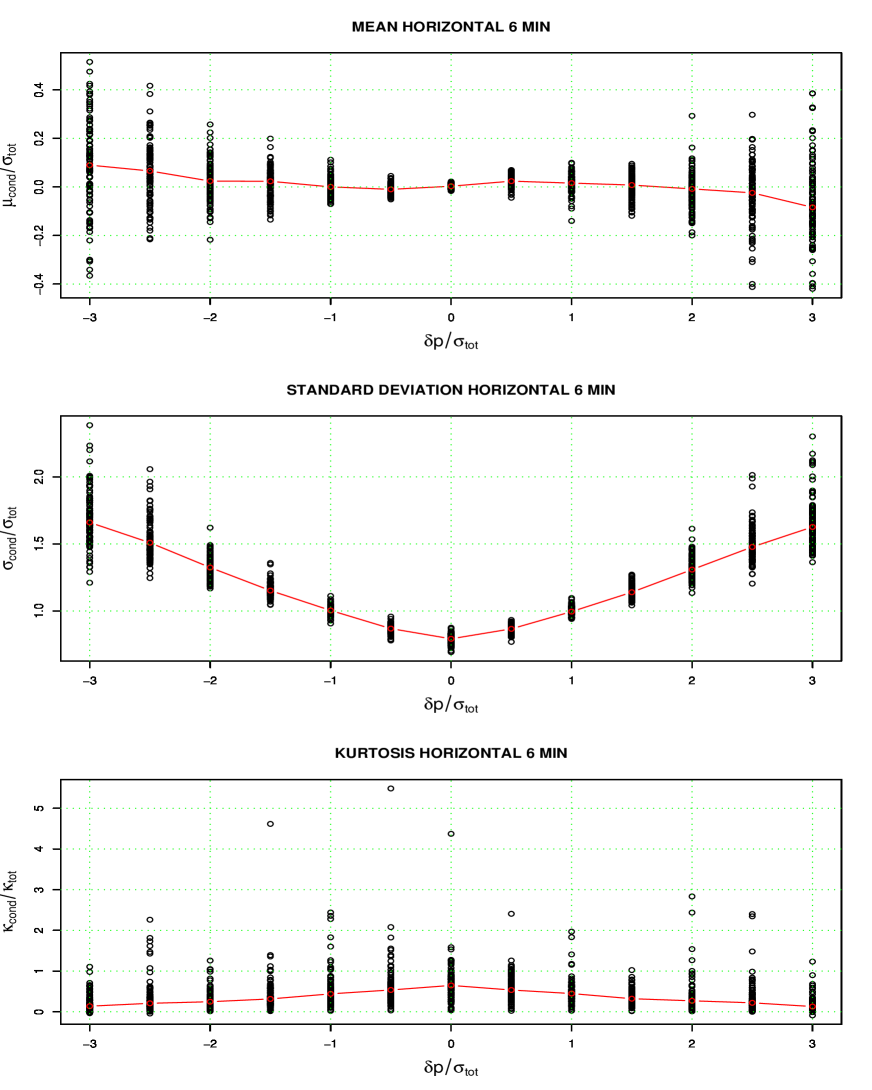
Figure 1: Normalized mean, standard deviation and anomalous kurtosis of the coarse-grained ”horizontal” conditional distribution versus the initial push, $\tau=6\,{\rm min}$, 100 stocks. Red lines show the medians of the scatterplots.

Let us now turn to the analysis of the ”vertical” interrelations between simultaneous price increments of different stocks The corresponding coarse-grained conditional distribution is constructed in complete analogy with the above-described ”horizontal” case:

$${\cal P}_{\Delta_{i}}(y^{j})\equiv{\cal P}(y^{j}|\,x^{k}\in\Delta_{i})\,,$$ (2)

where the conditioned variable $x^{k}\equiv\delta p^{k}(t)/\sigma^{k}_{\rm tot}$ refers to the $k$-th stock, and the response variable $y^{j}\equiv\delta p^{j}(t)/\sigma^{j}_{\rm tot}$ - to the $j$-th one.

In Fig. 2 we show the normalized conditional mean, standard deviation and kurtosis for 6-min. intervals for the ”vertical”case.

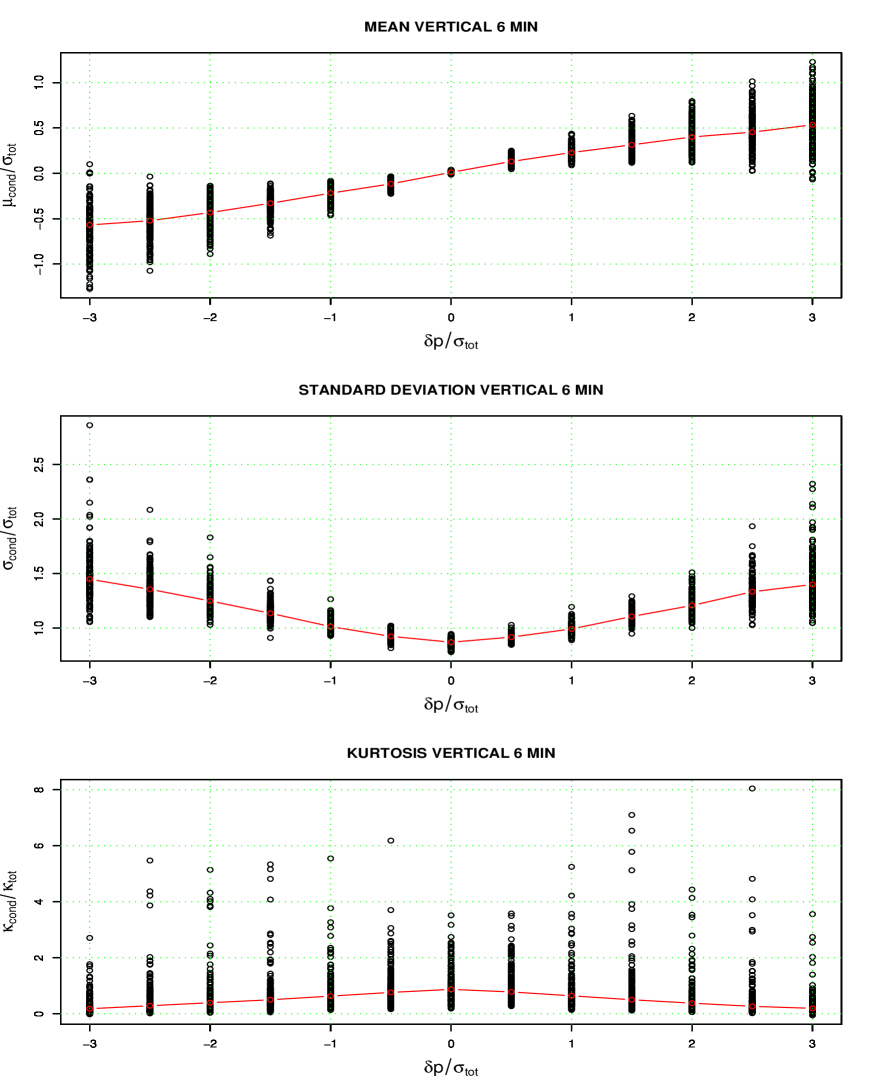
Figure 2: Normalized mean, standard deviation and anomalous kurtosis of the coarse-grained ”vertical” conditional distribution versus the initial push, $\tau=6\,{\rm min}$ , 100 stocks. Red lines show the medians of the scatterplots.

In Fig. 3 we plot the medians of the scatterplots for the normalized conditional mean, standard deviation and kurtosis for 6-min. and 60-min. intervals, combining the ”horizontal” and ”vertical” quantities.

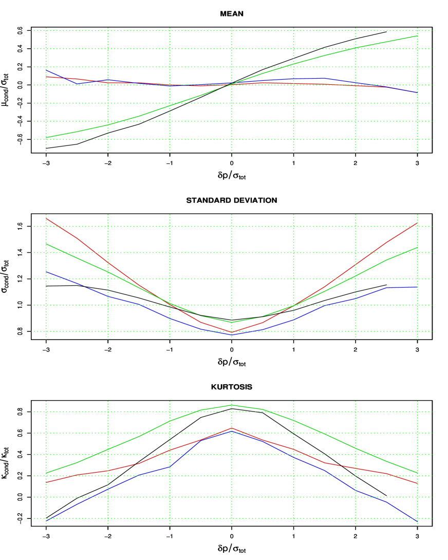
Figure 3: Medians of normalized mean, standard deviation and anomalous kurtosis of the coarse-grained conditional distribution versus the initial push, $\tau=6\,{\rm min}$ (”horizontal”: red line, ”vertical”: blue line) and $\tau=60\,{\rm min}$ (”horizontal”: green line, ”vertical”: black line).

The analysis of Figs. 1, 2 and 3 leads to the following conclusions:

• The resulting plots for conditional mean $\mu_{{\rm cond}}$ in the ”horizontal” case are too noisy to allow unambiguous interpretation. In the ”vertical” case one observes, for both cases of $\tau=6\,{\rm min}$ and $\tau=60\,{\rm min}$, a picture consistent with that of conditional mean generated through the presence of positive correlation, see below Eqs. (3) and (3).

• The plots of the relative conditional standard deviation $\sigma_{{\rm cond}}$ in ”horizontal” and ”vertical” case are, for the both cases of $\tau=6\,{\rm min}$ and $\tau=60\,{\rm min}$, strikingly similar. For $\tau=6\,{\rm min}$ we observe a pronounced conditional volatility smile, or dependence-induced volatility smile (D-smile) (see a more detailed discussion of this phenomenon in the next section), such that at small $x$ the standard deviation of the response is smaller than the unconditional standard deviation, while in the tails it is, on contrary, larger. For $\tau=60\,{\rm min}$ the smile is noticeably flatter than for $\tau=6\,{\rm min}$. This effect can be explained by the decay of anomalous kurtosis of price increments with growing $\tau$, see below discussion after Eq. (3).

• The median conditional kurtosis is noticeably smaller than the unconditional one.

We see, that in both ”vertical” and ”horizontal” cases the data shows, for both scales of $\tau=6\,{\rm min}$ and $\tau=60\,{\rm min}$, the same rather nontrivial patterns: conditional volatility smile and decrease of conditional kurtosis. The origin of the first effect is discussed in the next section. We shall argue, that it is in the probabilistic dependence of the adjacent price increments, whereas the role of linear correlation effects is in fact minor.

3 Model

Let us now present a model that explains the phenomenona of dependence-induced volatility smile and kurtosis reduction in the coarse-grained conditional distributions described in the previous section.

At the fundamental level of description the model describing the behavior of $N$ securities in two adjacent time intervals is fully specified by a $2N$ - dimensional probability distribution. The focus of our study is on the properties of the conditional distributions constructed from this basic enveloping $2N$-dimensional distribution. Generically conditional distributions are obtained by restricting the values of a subset of variables. Let us collectively denote these variables by ${\bf x}$, where ${\bf x}$ is a $N_{\bf x}$ - dimensional vector. Generically the vector ${\bf x}$ can include increments belonging to different time intervals. We are thus dealing with a conditional distribution depending on $N_{\bf y}\equiv 2N-N_{\bf x}$ variables. If we stay within the class of elliptical distributions, the multivariate probability distribution is a function of a quadratic form ${\cal K}$ constructed from the vector ${\bf z}^{\top}=({\bf y},{\bf x})$ and the generalized covariance matrix $\Sigma$, ${\cal K}={\bf z}^{\top}\cdot\Sigma^{-1}\cdot{\bf z}$. The covariance matrix $\Sigma$ includes the $N_{\bf x}\times N_{\bf x}$ covariance matrix $C_{\bf x}$ describing the correlations within the subset of conditioned variables ${\bf x}$, the $N_{\bf y}\times N_{\bf y}$ covariance matrix $C_{\bf y}$ describing the correlations within the subset of the variables ${\bf y}$ and the $N_{\bf x}\times N_{\bf y}$ covariance matrix $C_{\bf xy}$ describing the cross-covariances between the two groups:

$$\Sigma=\left(\begin{array}[]{cc}C_{\bf y}&C_{\bf xy}\\ C_{\bf xy}^{\top}&C_{\bf x}\end{array}\right)$$ (3)

At this stage we have to give an explicit description of the multivariate distribution containing the covariance matrix $\Sigma$. As will be elucidated below, a simplest choice of a gaussian multivariate distribution does not allow to explain the phenomena of D-smile and kurtosis reduction. There is, therefore, a clear need of taking into account the non-gaussian effects. The simplest possibility of keeping a fat-tailed nature of the probability distributions of individual increments is to construct a multivariate distribution from the fat-tailed marginals. Recombination of these marginals into a multivariate distribution requires constructing an appropriate copula. This construction is not unique, so the choice is guided by simplicity and ability to reproduce basic features of market data [12, 13]. In what follows we will show that a multivariate t-Student distribution makes a good job in this respect, while the Gaussian multivariate distribution fails to reproduce the properties of conditional distributions observed in market data.

Let us consider a $2N$-dimensional t-Student distribution

$$P^{(2N)}_{S}\,=\,\frac{1}{\sqrt{(\pi\mu)^{2N}\xi_{\mu}^{2N}{\rm det}\Sigma}}\,\frac{\Gamma\left(\frac{\mu+2N}{2}\right)}{\Gamma\left(\frac{\mu}{2}\right)}\left[1+\frac{1}{\mu}\frac{1}{\xi_{\mu}}{\bf z}^{\top}\,\Sigma^{-1}\,{\bf z}\right]^{-\frac{\mu+2N}{2}}.$$ (4)

where $\xi_{\mu}=(\mu-2)/\mu$ is a normalization factor ensuring, in particular, that the covariances computed with the distribution (4) are equal to the corresponding matrix elements of the matrix $\Sigma$.

Fixing some particular configuration of the ”initial” increments ${\bf x}={\bf x_{0}}$ leads to the conditional distribution (see, e.g., [14]):

$$P^{(N)}_{S}({\bf y|\,x_{0}}) = \frac{1}{\sqrt{(\pi(\mu+N_{\bf x}))^{N_{\bf y}}\xi_{\mu+N_{\bf x}}^{N_{\bf y}}{\rm det\Sigma_{{\bf y|\,x_{0}}}}}}\,\frac{\Gamma\left(\frac{\mu+N_{\bf x}+N_{\bf y}}{2}\right)}{\Gamma\left(\frac{\mu}{2}\right)}$$ (5)

$$\times \left[1+\frac{1}{\mu+N_{\bf x}}\frac{1}{\xi_{\mu+N_{\bf x}}}({\bf y}-\langle{\bf y}\rangle_{\bf x_{0}})^{\top}\,\Sigma_{\bf y|\,x_{0}}^{-1}\,({\bf y}-\langle{\bf y}\rangle_{\bf x_{0}})\right]^{-\frac{\mu+N_{\bf x}+N_{\bf y}}{2}}.$$

The conditional distribution (5) is a multivariate $N_{\bf y}$ - dimensional t-Student distribution with the index $\mu+N_{\bf x}$ and the following expected mean and covariance matrix:

$$\langle{\bf y}\rangle_{\bf x_{0}} = C_{\bf xy}C_{\bf x}^{-1}\,{\bf x_{0}}$$

$$\Sigma_{\bf y|\,x_{0}} = \left(C_{\bf y}-C_{\bf xy}C_{\bf x}^{-1}C_{\bf xy}^{\top}\right)\left[\frac{\mu-2}{\mu+N_{\bf x}-2}\right]\,\left[1+\frac{1}{\mu}\frac{1}{\xi_{\mu}}{\cal K}_{\bf x_{0}}\right]\,,$$ (6)

where ${\cal K}_{\bf x_{0}}={\bf x_{0}}^{\top}C_{\bf x}^{-1}{\bf x_{0}}$. Let us note, that if we had used the Gaussian multivariate distribution for constructing the conditional distribution analogous to (5), we would obtain a Gaussian conditional distribution with the following expected mean and covariance matrix:

$$\langle{\bf y}\rangle_{\bf x_{0}}^{G} = C_{\bf xy}C_{\bf x}^{-1}\,{\bf x_{0}}$$

$$\Sigma_{\bf y|\,x_{0}}^{G} = C_{\bf y}-C_{\bf xy}C_{\bf x}^{-1}C_{\bf xy}^{\top}$$ (7)

Comparing Eqs. (3) and (3) we see, that the expected mean is in both cases the same, whereas the expected variance in the t-Student case is a product of the gaussian expression and a $\mu$- and ${\cal K}_{\bf x}$ - dependent factor. An additional important phenomenon in the case of a t-Student distribution is an increase of the tail exponent determining the fat-tailedness of the distribution: $\mu\Rightarrow\mu+N_{\bf x}$ that thereby reduces the anomalous kurtosis

$$\kappa=\frac{6}{\mu-4}\,\,\,\,\,\Longrightarrow\,\,\,\,\,\kappa=\frac{6}{\mu+N_{\bf x}-4}$$ (8)

To describe the conditional volatility smile phenomenon discussed in the previous section, one clearly needs initial conditions’ depending covariances. From the formula (3) we see that in the Gaussian case this effect is absent, whereas for t-Student distribution the required dependence is manifest (see the second expression in (3) containing the factor of $\left[1+\frac{1}{\mu}\frac{1}{\xi_{\mu}}{\cal K}_{\bf x_{0}}\right]$). Of course, one should still prove that this dependence allows to describe the market data, see below. Nevertheless, already at this stage of our analysis, one can conclude that the phenomenon of conditional volatility smile can be explained only by non-gaussian effects - simply because the gaussian formalism does not have room for its description.

The conditional distribution Eq. (5) summarizes the impact the ”initial” configuration ${\bf x_{0}}$ has on the ”final” one ${\bf y}$.

The explanation of the conditional volatility smile and kurtosis reduction effects described in the previous section requires a simpler $2$-dimensional version of (4) with one-dimensional $y$ and $x$. Let us thus consider two price increments in the two consecutive time intervals for the same stock for the ”horizontal” case (or the simultaneous increments of two stocks for the ”vertical” case) and introduce the corresponding bivariate distribution

$$P^{(2)}_{S}(y,x)\,=\,\frac{1}{\sqrt{(\pi\mu)^{2}\xi_{\mu}^{2}{\rm det}\Sigma}}\frac{\Gamma\left(\frac{\mu+2}{2}\right)}{\Gamma\left(\frac{\mu}{2}\right)}\frac{1}{\left(1+\frac{1}{\mu}\frac{1}{\xi_{\mu}}K_{\Sigma}(x,y)\right)^{\frac{\mu+2}{2}}}$$ (9)

Here $\Sigma$ is a covariance matrix

$$\Sigma\,=\,\begin{pmatrix}\sigma_{y}^{2}&\sigma_{x}\sigma_{y}r\\ \sigma_{x}\sigma_{y}r&\sigma_{x}^{2}\end{pmatrix}$$ (10)

and $K_{\Sigma}=(y,x)\cdot\Sigma^{-1}\cdot(y,x)^{\top}$ The conditional distribution ${\cal P}(y|\,x=x_{0})$ corresponding to the above distribution is again a t-Student distribution with the tail exponent $\mu+1$, conditional mean $\langle y\rangle_{x_{0}}$ and conditional $x_{0}$ - dependent variance $\sigma^{2}_{y|x_{0}}$

$$\langle y\rangle_{x_{0}} = r\,x_{0}$$

$$\sigma_{y|x_{0}}^{2} = \sigma_{y}^{2}(1-r^{2})\,\frac{\mu-2}{\mu-1}\left(1+\frac{1}{\mu}\frac{1}{\xi_{\mu}}\frac{x_{0}^{2}}{\sigma_{x}^{2}}\right)$$ (11)

Therefore the conditional distribution is more gaussian (the ratio of its anomalous kurtosis to the unconditional one is equal to $(\mu-4)/(\mu-3)<1$), but its standard deviation can be smaller or larger than the unconditional value $\sigma_{y}$ depending on the value of the conditioned variable $x_{0}$. The parabolic dependence of the conditional volatility on the initial push $x_{0}$ is just the feature we need to explain the D-smiles in Figs. 1, 2 and 3. The fine structure we have observed – namely, the flattening of the D-smile with growing $\tau$, can also be explained with the help of Eq. (3). Indeed, the coefficient at $x_{0}^{2}$ is equal to $1/(\mu\xi_{\mu})\equiv 1/(\mu-2)$. Now the data shows (see below Fig. 4) that for larger time intervals the unconditional anomalous kurtosis $\kappa_{\tau}$ is smaller, and the tail index $\mu_{\tau}=4+6/\kappa_{\tau}$ is, correspondingly, larger, leading to the desired flattening of the smile. The unconditional anomalous kurtosis $\kappa_{\tau}$ and the corresponding tail index $\mu_{\tau}$ are plotted for the ensemble of $N=100$ stocks considered in the paper for several intraday time intervals, in Fig. 4.

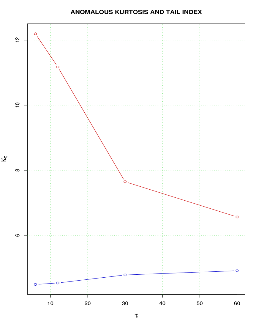
Figure 4: Unconditional anomalous kurtosis $\kappa_{\tau}$ (red line) and corresponding tail index of the t-Student distribution $\mu_{\tau}$ (blue line) for several intraday time intervals $\tau$.

Let us also note that in the gaussian case one has $\langle y\rangle_{x}=r\cdot x_{0}$ and $\sigma_{y|x_{0}}^{2}=\sigma_{y}^{2}(1-r^{2})$ so, as has been already mentioned, the gaussian probabilistic link between the price increments does not leave room for $x_{0}$ - dependent effects in the conditional covariance matrix.

To make the correspondence with the market data quantitative we should, however, introduce a coarse-grained version of the conditional distribution ${\cal P}(y|\,x\in\Delta)$, where the variable $x$ belongs to a certain subinterval $\Delta$:

$${\cal P}(y|\,x\in\Delta)\,=\,\frac{\int_{x\in\Delta}dx\,P^{(2)}_{S}(y,x)}{\int_{x\in\Delta}dx\,P_{S}^{(1)}(x)}$$ (12)

We have computed the normalized mean, relative standard deviation and anomalous kurtosis of a set of conditional distributions corresponding to the same coarse-graining of the increments $x\equiv\delta p(t)/\sigma_{\rm tot}$ as used in the analysis of the market data in the previous section, tail index $\mu=5$ and a set of correlation coefficients $r=0.25,0.5,0.75$. The conditional mean is, of course, simply proportional to $x_{0}$. The conditional kurtosis drops to the expected $\kappa=3$, with small deviations. Most interesting is, of course, the behavior of the conditional standard deviation shown in Fig. 5.

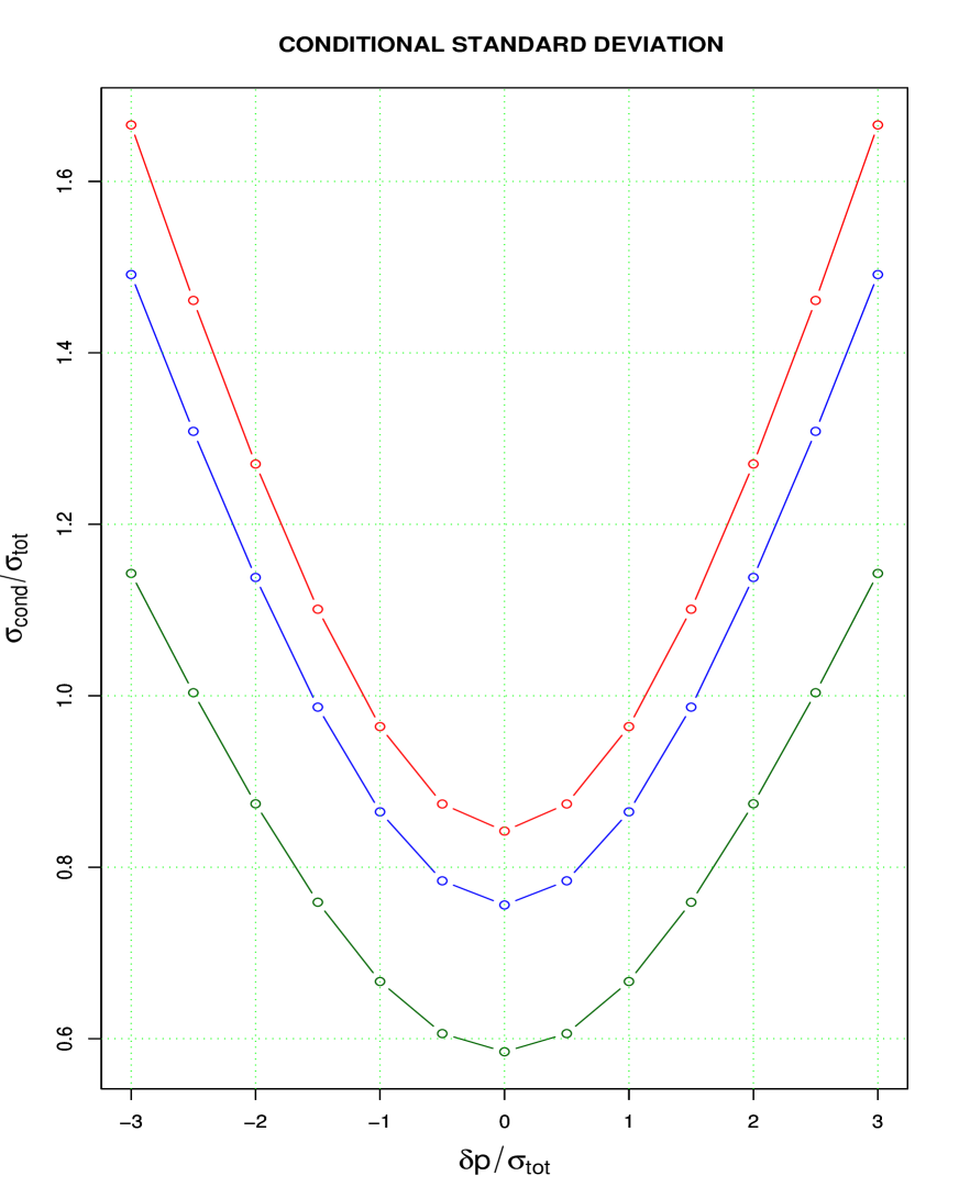
Figure 5: Normalized standard deviation of the model coarse-grained conditional distribution versus the initial push; red: $r=0.25$, blue: $r=0.5$, green; $r=0.75$

We see that the model reproduces the conditional volatility smile with characteristics very similar to those observed in the market data.

A crucial point in the correct interpretation of the above result is that linear correlation (present through the correlation coefficient $r$) shows itself only via setting the absolute scale for the variance, see the second of Eq. (3). It is clear,that the conditional volatility smile would be present even in the complete absence of correlations ($r=0$). Therefore it is really appropriate to call the volatility dependence in question a dependence-induced volatility smile (D-smile). Considering for instance the ”horizontal” case, the probabilistic dependence between the increments $\delta p(t)$ and $\delta p(t+1)$ can be manifestly demonstrated by computing, e.g., the correlator of their absolute values $G(1)=\langle|\,\delta p(t)|\cdot|\,\delta p(t+1)|\rangle_{t}-(\langle|\,\delta p|\rangle_{t})^{2})$. Calculating this correlator for the bivariate t-Student distribution (9) and its Gaussian counterpart gives

$$G_{G}(1) = \frac{2}{\pi}\,\sigma_{\rm tot}^{2}\,r^{2}\,\left(\sqrt{1-r^{2}}+\frac{\rm{Arcsin}\,r}{r}\right)$$ (13)

$$G_{S}(1) = \frac{\mu}{\pi}\,\sigma_{\rm tot}^{2}\left[\frac{\Gamma\left(\frac{\mu-2}{2}\right)\Gamma\left(\frac{\mu}{2}\right)-\Gamma^{2}\left(\frac{\mu-1}{2}\right)}{\Gamma^{2}\left(\frac{\mu}{2}\right)}\right]+$$ (14)

$$\frac{\mu}{\pi}\,\sigma_{\rm tot}^{2}\frac{\Gamma\left(\frac{\mu-2}{2}\right)}{\Gamma\left(\frac{\mu}{2}\right)}\,r^{2}\,\left[\sqrt{1-r^{2}}+\frac{\rm{Arcsin}\,r}{r}\right]$$

In the gaussian case the (linearly) uncorrelated variables are also independent and, indeed, the correlator (13) vanishes as $r^{2}$ at $r\to 0$. In the case of t-Student distribution the correlator (14) is, on contrary, nonzero at $r=0$, so increments are in this case probabilistically dependent. Let us stress that this dependence is in fact imposed by the form of the unconditional distribution we have chosen. One crucial feature is that the t-Student distribution ensures, in agreement with observations, that the corresponding marginal distributions are fat-tailed. The t-Student copula we have used provides a framework in which the dependence effects are present even in the complete absence of linear correlations.

4 Discussion

There still remains a number of important issues related to the questions discussed in the paper that we leave for the future analysis [15].

First, one would like to generalize the binary-level description of simultaneous ”vertical” interdependence of stock price increments to the fully multivariate case of the influence of the $n$-point ”trigger” configuration $\{\delta p_{j}(t)\}$ on the move of the $k$-th stock in the next time interval $\delta p_{j}(t+\tau)$.

Second, perhaps more difficult issue is studying the properties of the conditional distributions for arbitrary separation of corresponding time intervals. Preliminary analysis of the market data shows the dependence of D-smile on this separation (”maturity”). This is to be expected from the fact that volatility autocorrelations decay, albeit slowly, with time. This forces to generalize the formalism we have used. In any case, a big goal is to establish connection with the explicit models of volatility dynamics, see e.g. [16, 17], including the leverage effects [4].

Finally, we would like to analyze in more details application of the nonlinear patterns we have described to portfolio optimization problems. Expected mean, volatility and degree of fat-tailedness are crucial ingredients of portfolio optimization schemes [4, 7], so specific effects related to them are of clear interest in this context.

5 Conclusion

Let us summarize the main results of the present paper.

The focus of our analysis is on the properties of conditional distributions characterizing the probabilistic behavior of an ensemble of financial instruments. The analysis of market data in the simplest case of a binary probabilistic dependence has revealed two major effects:

• The smile-shaped dependence of conditional volatility on the magnitude of the input due to non-gaussian nature of the enveloping t-Student distribution

• A noticeable reduction of the conditional anomalous kurtosis as compared to the unconditional one

Let us also mention the flattening of the D-smile with growing time interval on which the price increments are computed.

We have constructed an explicit model characterizing the collective probabilistic pattern of an ensemble of price increments that gives a natural explanation of the above-listed phenomena. The model is based on a multinomial t-Student distribution. This theoretical framework allows to unambiguously relate the effects of a dependence-induced volatility smile and kurtosis reduction to the non-gaussian nature of the eneveloping distribution.

Acknowledgements

The authors are very grateful to Eugene Pinsky for discussions and comments.

The work of A.L. was supported by the RFBR Grant 04-02-16880, and the Scientific school support grant 1936.2003.02

6 Appendix

Below we give a list of stocks studied in the paper:

A, AA, ABS, ABT, ADI, ADM, AIG, ALTR, AMGN, AMD, AOC, APA, APOL, AV, AVP, AXP, BA, BBBY, BBY, BHI, BIIB, BJS, BK, BLS, BR, BSX, CA, CAH, CAT, CC, CCL, CCU, CIT, CL, COP, CTXS, CVS, CZN, DG, DE, EDS, EK, EOP, EXC, FCX, FD, FDX, FE, FISV, FITB, FRE, GENZ, GIS, HDI, HIG, HMA, HOT, HUM, JBL, JWN, INTU, KG, KMB, KMG, LH, LPX, LXK, MAT, MAS, MEL, MHS, MMM, MO, MVT, MX, MYG, NI, NKE, NTRS, PBG, PCAR, PFG, PGN, PNC, PX, RHI, ROK, SOV, SPG, STI, SUN, T, TE, TMO, TRB, TSG, UNP, UST, WHR, WY

References

- [1] B. Mandelbrot, ”Fractal and Multifractal Finance. Crashes and Long-dependence”, www.math.yale.edu/mandelbrot/webbooks/wb_fin.html
-
[2]
A.C. MacKinlay, A.W. Lo, J.Y. Kampbell, The Econometrics of Financial Markets, Princeton, 1997;
A.W. Lo, A.C. MacKinlay, A Non-Random Walk Down Wall Sreet, Princeton, 1999 - [3] R.N. Mantegna, H.E. Stanley, An Introduction to Econophysics, Cambridge, 2000.
- [4] J.-P. Bouchaud, M. Potters, Theory of Financial Risk and Derivative Pricing, Cambridge, 2000, 2003.
- [5] R. Cont, ”Empirical properties of asset returns: stylized facts and statistical issues”, Quantitative Finance 1 (2001), 223
-
[6]
F. Lillo, R. Mantegna, ”Symmetry alteration of ensemble return distribution in crash and rally days”,
arXiv:cond-mat/0002438;
”Ensemble properties of securities traded in the NASDAQ market”, Proceedings of NATO ARW on Application of Physics in Economic Modelling, Prague, 8-10 February 2001, arXiv:cond-mat/0107256 - [7] E. Elton, M. Gruber, S. Brown, L. Stern, Modern Portfolio Theory and Investment Analysis, John Wiley, 2003
- [8] A. Lo, A. MacKinlay, ”When Are Contrarian Profits Due to Stock Market Overreaction?”, Review of Financial Studies 3 (1990), 175-208
- [9] M. Boguna, J. Masoliver, ”Conditional dynamics driving financial markets”, arXiv:cond-mat/0310217
- [10] K. Chen, C. Jayprakash, B. Yuan, ”Conditional Probability as a Measure of Volatility Clustering in Financial Time Series”, arXiv:physics/0503157
-
[11]
E. Alessio et.al., ”Multivariate distribution of returns in financial time series”,
Proceedings of the International Conference of Computational Methods in Sciences and Engineering 2003 (ICCMSE 2003),
Ed. T.E. Simos (World Scientific Publishing Co., Singapore, 2003), pp. 323-326 [ArXiv:cond-mat/0310300];
E. Alessio et.al., ”Modeling stylized facts for financial time series”, Physica A 344, 263-266 (2004) [ArXiv:cond-mat/0401009] - [12] Y. Malevergne, D. Sornette, ”Testing the Gaussian Copula Hypothesis for Financial Assets Dependences”, Quantitative Finance 3 (2003) 231-250 [arXiv:cond-mat/0203166]
- [13] W. Breymann, A. Dias and P. Embrechts, ”Dependence structures for multivariate high-frequency data in finance”, Quantitative Finance 3 (2003), 1-14.
- [14] G. Box, G. Jenkins, ”Time Series Analysis. Forecasting and Conrol”, Holden-Day, 1970
- [15] A. Leonidov, V. Trainin, A. Zaitsev, work in progress
- [16] B. LeBaron, ”Stochastic Volatility as a Simple Generator of Financial Power-laws and Long Memory”, Quantitative Finance 1 (2001), 631
- [17] G. Zumbach, ”Volatility processes and volatility forecast with long memory”, Olsen research report, www.olsen.ch