On Multifractal Structure in Non-Representational Art J. R. Mureika
Email: jmureika@lmu.edu
Department of Physics, Loyola Marymount University, Los Angeles, CA  90045-8227
C. C. Dyer
Email: dyer@astro.utoronto.ca
Department of Astronomy and Astrophysics, University of Toronto, Ontario, Canada
G. C. Cupchik
Email: cupchik@scar.utoronto.ca
Division of Life Sciences, University of Toronto at Scarborough, Ontario, Canada

Abstract
Multifractal analysis techniques are applied to patterns in several abstract expressionist artworks, paintined by various artists. The analysis is carried out on two distinct types of structures: the physical patterns formed by a specific color (“blobs”), as well as patterns formed by the luminance gradient between adjacent colors (“edges”). It is found that the analysis method applied to “blobs” cannot distinguish between artists of the same movement, yielding a multifractal spectrum of dimensions between about $1.5-1.8$. The method can distinguish between different types of images, however, as demonstrated by studying a radically different type of art. The data suggests that the “edge” method can distinguish between artists in the same movement, and is proposed to represent a toy model of visual discrimination. A “fractal reconstruction” analysis technique is also applied to the images, in order to determine whether or not a specific signature can be extracted which might serve as a type of fingerprint for the movement. However, these results are vague and no direct conclusions may be drawn.

PACS Primary: 89.75.Da; secondary: 95.75.mN; tertiary: 89.75.Kd

1 Introduction and Background

The use of fractal analysis methods to study structure in art and music is not a new field. Recently, the question of perceptability of such fractal structure has been addressed. The authors of References [1, 2] pose the question of whether or not humans are “attuned” to the perception of fractal-like optical and auditory stimuli. Similarly, [3] suggests that there is a fractal-like signature in memory processes which can be detected in the statistical variance of averaged repeated actions (such as repeated drawing lines of specific lengths or shapes; the statistical variations in the lengths are shown to be not purely random noise, but fractally ordered “$1/f$” noise).

In the visual arts, there have been several contributions made by the authors of [4, 5, 6, 7], in which the paintings of Jackson Pollock play a prominent role. Of their many interesting conclusions, the most striking is that Pollock’s drip paintings almost uniformly possess a fractal dimension around 1.7. This was confirmed by the authors of [8, 9], who also extended the study to other artists of the abstract expressionist school (notably the Québec-based group Les Automatistes). It was discovered that many of the paintings from these other artists possess a similar fractal dimension.

Similar research on computer-generated cosmological models suggests that the fractal (or box) dimension is a vague statistic for identifying structural differences in point sets, and that the full multifractal spectrum can yield deeper information as to the nature of the distributions [10]. However, it has been concluded that the utility of the method seems limited to identifying classes of distributions formed by different mechanisms, and not differences between individual members of the same class.

In the following paper, this method will be applied to two-dimensional, non-representational images, to ascertain whether or not similar statements may be made about the analysis. Summary results of this study have been reported in Reference [9], but this paper will greatly expand upon the data and present technical details of the analysis in diverse ways. An overview of fractal and multifractal theory is first presented. Following this, the fractal (box) dimension for several abstract expressionist paintings by different artists is performed, and this is contrasted with the information dimension for the same works. The box method is tested for robustness in Section 5.

As a control, these abstract expressionist are contrasted with the deterministic “Artonomy” paintings by Tsion Avital [11]. Like the three dimensional distributions, the two former works can be interpreted to be formed by one type of mechanism (although the comparison is perhaps more ambiguous), while the latter a decidedly different mechanism (this differentiation will be further discussed in Section 8).

The analysis will then be extended to include the full multifractal spectrum for each work. A comprehensive analysis is performed on color patterns for the artists in question, beginning in Section 7. Furthermore, issues addressing potential image reconstruction from the multifractal spectrum is discussed in Section 9. Finally, as a toy model for visual discrimination based on the notion that human perception may be influenced by contrast edges instead of colors, the multifractal spectra of contrast patterns in the paintings are analyzed in Section 10. Some limitations of the method are discussed in Section 11, and concluding remarks are summarized in Section 12.

2 Theory of Multifractals

The similarity in form and function of the classic fractal (or box) dimension, Shannon’s information dimension, and the statistical correlation dimension is not a coincidence (see References [12, 13, 14, 15] for general details on these dimensions). In fact, these quantities are but three members of an infinite set of dimensions which characterize a fractal set. Since first being introduced as a method of describing or quantifying the behavior of strange attractor sets and turbulent flows, multifractal analysis has gained steady momentum in physics and fields abroad [16, 17, 18, 19, 20]. Comprehensive reviews of multifractals and their applications in the physical sciences are available in the aforementioned references, as well as such works as [21, 22, 23], in addition to many of the references cited hereafter.

Classic geometric “monofractals” such as the Koch snowflake or Sierpinski carpet are defined by a single scale invariant behavior, which of course is the fractal dimension, but in many cases a single such power law fails to characterize completely the distribution in question. Multifractals, on the other hand, may be regarded as an intricate weave of an infinite number of fractals, all of which are characterized by different (local) scaling dimensions. That is, each subset forms a “sub-fractal” describing a distinct sub-structure of the whole. It is much more reasonable and realistic to expect natural objects to exhibit this behavior.

Multifractal dimensions are generalizations of the Hausdorff measure [13]. The partition function for an $\epsilon$-covering (i.e. balls of radius $\epsilon_{i}$) is defined as [17, 20]

$$\Gamma(q,\tau)=\sum_{i}\frac{p_{i}^{q}}{\epsilon_{i}^{\tau}}~{},$$ (1)

with $p_{i}$ a measure of the set or pattern density in the ball. For given $q,\tau(q)\in{\cal R}$, take the supremum (or infimum, depending on whether $q$ is positive or negative, respectively) in the limit $\epsilon_{i}\rightarrow 0$ (thus find the minimal covering set for the generalized measure). Then, there exists a critical value of $\tau\equiv\tau(q)$ for which $\Gamma(q,\tau)$ goes from convergence to 0, to divergence to $\infty$. At this transitionary value, the sum converges as $\Gamma(q,\tau)={\rm const}$. The minimal covering may be generalized to balls of equal radii $\epsilon_{i}=\epsilon$, whence it follows that

$$\Gamma(q,\tau)=\epsilon^{-\tau(q)}\sum_{i}p_{i}^{q}\sim 1~{},$$ (2)

for a suitable renormalization of the measure. Hence,

$$\sum_{i}p_{i}^{q}\sim\epsilon^{\tau(q)}~{},$$ (3)

and thus in the limit $\epsilon\rightarrow 0$, it can be shown that

$$\tau(q)=\lim_{\epsilon\rightarrow 0}\frac{\log[\sum_{i}p_{i}^{q}]}{\log\epsilon}~{}.$$ (4)

Let the measure partition function over $N(\epsilon)$ balls of radius $i$ be

$$Z(q,\epsilon)=\sum_{i=1}^{N(\epsilon)}\;[p_{i}(\epsilon)]^{q}~{},$$ (5)

and define the general scaling relation $Z(q,\epsilon)\sim\epsilon^{(q-1)\;D_{q}}$ [23], which ensures recovery of the Hausdorff dimension for $q=0$, as well as normalization of (5) for $q=1$. From (4), it can be concluded that

$$D_{q}=\frac{\tau(q)}{q-1}~{}.$$ (6)

In the limit $q\rightarrow 0$, (1) reduces to the usual box dimension. Furthermore, the information and correlation dimensions are recovered in the limits $q\rightarrow 1,2$.

In practical applications, the box counting method can be generalized to obtain the values of $\tau(q)$ for given $q$. That is, modify the partition function $Z(q,\epsilon)$ over $N(\epsilon)$ to sets of covering boxes (instead of balls) of equal side $\epsilon$, where as before $p_{i}(\epsilon)$ is the relative density of the set in box $i$. The scaling information of each moment is obtained by taking the logarithmic derivative of (5) with respect to box size, where

$$\tau(q)=\frac{d\log[Z(q,\epsilon)]}{d\log(\epsilon)}~{}.$$ (7)

The moment parameter $q$ can be thought of as a filter, which identifies only the singularity characteristics of the distribution at a particular “degree” of clustering. Increasing values of $q>0$ emphasize the stronger local clustering nature of the pattern, while decreasing values of $q<0$ the less singular regions. That is, higher values of $q$ serve to “eliminate” the smaller values of $p_{i}$, yielding a subset of the overall distribution whose scaling behavior is more condensed (and vice versa for negative $q$). Likewise, the other $D_{q}$ provide a measure of the number of q-tuples whose mutual separation is contained within a covering box (ball) of size $\epsilon$. Thus, a quantitative measure of the $D_{q}$ spectrum yields an understanding of all order of correlations amongst clusters of varying densities.

Certain key values of $D_{q}$ are extremely useful in characterizing the physical clustering characteristics of a set. In addition to the values $D_{0,1,2}$ mentioned before, the generalized dimensions for the limits $q\rightarrow\pm\infty$ yield valuable information about the maximal and minimal density regions of the set. $D_{\infty}$ is a measure of the scaling behavior for the densest clustering regions of the multifractal, while $D_{-\infty}$ corresponds to the equivalent for the least dense or “rarefied” regions.

In essence, the multifractal measures give an indication of “how fractal is the fractal”. A measure of the difference between the box dimension and any successive $D_{q}$ value

$$\Delta=D_{q}-D_{0}~{}.$$ (8)

provides an estimate of the “degree” of inhomogeneity of the associated probability distribution [22]. In particular, it seems reasonable to evaluate $\Delta|_{q\rightarrow\infty}$ as an overall gauge of the “depth” of inhomogeneity. Clearly, it follows that $\Delta=0$ for single-scaling Euclidean normal or monofractal sets, so the larger the value of $\Delta$, the greater the “multifractality”.

3 Fractal Expressionism

In the last 1990s, the application of fractal analysis to the study of abstract expressionist art began to gain momentum, the first of which was reported in [5]. It was concluded that Jackson Pollock’s work did indeed present certain fractal characteristics. Coined “Fractal Expressionism”, the authors in question proposed that Pollock’s drip paintings were constructed by processes not unlike those which help to forge the myriad of similarly fractal natural phenomena. In fact, they further suggested that by painting with such “automatism”, Pollock succeeded in capturing the very essence of nature within his works.

In particular, it was noted that most of the paintings studied contain at least two distinct scaling behaviors at different levels, much the same as the debated transitions to homogeneity in galaxy clustering. The first of these occurred at scales on the order of 1 mm to about 5 cm, beyond which point a second scaling is observed up to scales of several meters [4]. After a review of Pollock’s painting methods and techniques, it was determined that these two dimensions were the result of two distinct physical processes. The larger-scale patterns resulted from Pollock’s “Levy flights” across the canvas (a Levy Flight is a combination of discrete, random jumps coupled with local fractal Brownian motion [23]). Likewise, the small-scale structure was attributed to his infamous “drip” technique, which was largely dependent on the physical characteristics of the paint (viscosity, the height from which it was dripped, absorption into the canvas, etc…).

These two dimensions are coined $D_{L}$ (Levy) and $D_{D}$ (Drip), and in general it was found that $D_{L}>D_{D}$ (in fact, the authors of [4] claim that $D_{L}$ tended to values close to 2, indicative of the “space-filling” behavior of Pollock’s Levy Flights). Furthermore, it was claimed that $D_{L}$ tended to increase from 1 to about 1.7 between the early 1940s to the late 40s / early 50s (around the time Pollock perfected his drip technique [24]).

Their analysis focused exclusively on the works of Jackson Pollock, and these dimensions are attribute to his own artistic style. In the spirit of the aforementioned conclusions of [10], however, the question should be asked as to whether or not such an analysis truly pinpoints anything “unique” about the artist in question, or whether the resulting statistics are shared by a common set of images and patterns formed by similar methods.

3.1 Image specifics

The majority of the images considered in this study are digital scans of Pollock’s works from the references [24, 25]. Images by Les Automatistes have been scanned from [26]. The resolution of the scans was chosen as 300 dpi, creating images roughly 1000 pixels (px) in length (longest side) and files 20 Mb in size. The analysis has been performed on approximately 25 Jackson Pollock paintings, revealing similar trends for each. However, this discussion will be restricted to a small sample set of six. The images herein are listed in Table 1. At the specified resolution, each pixel corresponds to approximately 0.1-0.4 cm, although this will depend on the actual reduction scale from the base image.

The covering boxes range in size from $d=$1024 px to $d=$4 px, or length scales of roughly $1.5-2.5~{}$m to a few millimeters. Hence, the analysis covers about 3 orders of magnitude. Higher resolutions could allow for greater range of scales, but would correspond to much larger images and longer run-times / higher memory requirements for the code. It was verified that the quality of the fits did not change appreciably for a lower limit of $d=2$, and the estimated dimensions were statistically equal to within the associated error.

3.2 Color Variance Filter Process

Accurate definitions of colors and color differences are very difficult to obtain. Any investigation which relies on color matching must do so with care. The following procedure is a rough example of how like colors might be extracted from an image, based on their Euclidean separation in the three dimensional RGB color space.

To trace or filter the pattern of a given pigment, the variation in shading is accounted for via the color-variance filter process. The images studied herein are 24-bit color maps, hence each separate channel may assume 256 possible values. An RGB triplet is chosen as the target color, each pixel (channel) intensity in the image is then compared to the initial triplets R₀, G₀, B₀ (hereafter RGB₀), and the Euclidean distance (or color radius) is calculated,

$$R_{RGB}=\sqrt{(R_{0}-R_{pix})^{2}+(G_{0}-G_{pix})^{2}+(B_{0}-B_{pix})^{2}}~{},$$ (9)

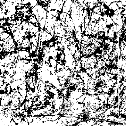
Figure 1: Black pigment filtered image P02, $\beta\sim 20$.

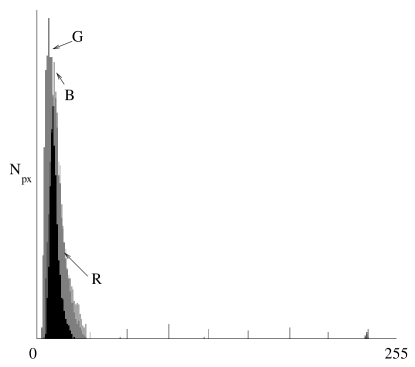
Figure 2: Pixel count $N_{\rm px}$ histogram for black pattern of P04, showing peaks at $(\rm{R},\rm{G},\rm{B})=(21,17,21)$.

Figure 1 shows the filtered pattern for $\beta_{RGB}=20$ for image P02. Patterns are isolated by including pixels for which $R_{RGB}\leq\beta$, a cutoff whose value is determined by examination of the RGB histogram for the color in question. Figure 2 shows the R, G, and B pixel intensity histogram for the “black” pigment of image P04, which is generally of the same form for all images considered herein. The peaks of each correspond roughly to the values $(\rm{R},\rm{G},\rm{B})=(21,17,21)$, which is taken as the target color RGB₀. Note the smooth drop-off for increasing (and decreasing) values of the pixel intensities.

For the paintings considered, it was found that most RGB histogram spreads tend to extend no more than 5-20 pixel intensities from the central peak. Hence, it seems reasonable to assume that the cutoff $\beta$ should be between $\beta\in(10\sqrt{3}-20\sqrt{3})\simeq(10,40)$.

The pseudo-normal nature of the distribution in Figure 2 suggests that a Gaussian filter, which weights colors according to their distance from the “target”, would be more appropriate that the cut-off filter considered presently. This type of filter is inappropriate for calculation of the box Dimension, for which any box is counted in which there exists a point in the allowable range (i.e. this would result in a severe over-count of boxes). However, a “weighted” information dimension is certainly feasible, in which one assigns the color match a value of $\rm{exp}(-R^{2}_{\,\rm{RGB}}/a^{2})$, with $a^{2}$ the FWHM corresponding to the average histogram spread. This filter would be better exploited in the multifractal analysis of 7. However, preliminary calculations suggest that the results will not vary significantly from those of the cut-off method described herein. Since the very notion of color distance discrimination itself is somewhat of a fuzzy area (see e.g. [27] or similar references), it is best not to “over-complicate” the procedure at this given stage of development. Thus, only the cut-off will be used in this study.

4 The Box and Information Dimension of Jackson Pollock’s Work

As previously mentioned, the information dimension can be considered a better statistic for the study of recursive patterns. That is, the box dimension can sometimes provide an overestimate of the scaling behavior, since it does not account for the relative density of points within the box. Although these specific results have been reported in [9], a slightly different analysis of the findings was given in that Reference. What follows will be a more technical discussion of the results.

Table 2 presents the corresponding dimension estimates for each painting. The Box Dimensions calculated by a least-squares regression on the data points seems to provide a good agreement to the results cited in [4], who found e.g. $D_{0}=1.67$ for P02 and 1.72 for P01. This suggests that a value of $\beta\in[20,30]$ would be in rough agreement with their analysis.

However, closer inspection of the results of Table 2 reveals that in certain cases the estimate of the dimension is critically dependent on a correct choice of $\beta$: the darker colors appear more stable, while the lighter ones show wider variation. In order for this analysis technique to be useful, these selection criteria must be extremely well defined. Otherwise, the results risk becoming meaningless. Ideally, some kind of variance in choice of $\beta$ should be incorporated into the overall error estimate. The issue of color space selection is discussed in Reference [28].

As mentioned in the previous section, the authors noted an apparent break in the slope of the log-log plot, and assumed that this represented different scaling behavior of two different mechanisms. The shallower slope was taken to be representative of Pollock’s painting technique. In fact, in reference [29], the author discusses the association of two distinct dimensions based on the topological morphology of the fractal (for higher length scales), as well as its texture (lower scales). These two dimensions are appropriately labeled as those of the structural fractal and textural fractal, respectively. Relating to the work of [4], it is not unreasonable to interpret their two dimensions accordingly, i.e. the overall “structure” of the painting at higher length scales, and the fine-grained refinement at lower scales.

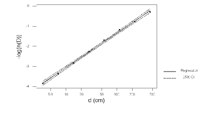
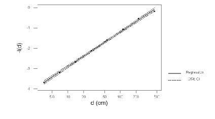
Figure 3: Sample log-log fits used to determine box and information dimensions for P02, $\ beta=20$.

Note that in the analysis presented herein, the two-slope hypothesis of [4] is not supported when one considers the magnitudes of the associated errors in the least-squares procedure. The confidence level curves suggest that the “shallow” slope at lower length scales could be explained as statistical variation in the fit. The fits in Figure 3 show box and information sample plots for P02 with 95% confidence level curves from the least-squares fit. The information Dimension $D_{1}$ is shown as a “refinement” of $D_{0}$, which demonstrates even less bi-scale behavior, suggesting that the two-slope hypothesis may be an artifact of the box-counting method. The data provides a very clean linear fit in both cases, generally better for the information dimension $D_{1}$, albeit not significantly ($r^{2}=99.9\%~{}vs~{}99.8\%$). Similar behavior is observed for the other images.

In fact, the lower-scale measurement process is somewhat dependent on the resolution of the image. Some of the fits suggest a shallower slope at smaller scale lengths, but it is not necessarily justified to assume that this behavior is an artifact of the pattern, and not the resolution of the image, or limitations of the counting/analysis method.

Although the methods herein and those of reference [4] differ interpretationally, roughly the same end result is obtained. That is, one can still associate an effective fractal dimension in the range $D_{0}\simeq 1.6-1.8$ with the patterns on the paintings, simply by considering the slope of the entire fit. A changing slope from box counting does not immediately imply multifractal behavior.

While it may be that the slope tends to be shallower at lower scales, this may not be an artifact of the data set so much as a manifestation of estimates and assumptions about the data. There may also be lower-level resolution limitations due to the finite size of the pixels. Surely, in the mapping from a 5 metre painting to a 30 cm page – or to a 1000 px binary image – there must be some significant level of information loss at the lower scales of resolution (in both the photograph and the data scanning process).

There does not seem to be significant variation in dimensions between lighter and darker colors, although in certain cases it is observed that the lighter pigment patterns tend to exhibit lower fractal dimensions. This could be due to a different deposition mechanism than simple dripping, as well. It is perhaps a sweeping generalization to assume that all the pigments were applied in exactly the same fashion.

So, it becomes somewhat unclear how one can define the “dimension” of the entire image. This suggests an application of the Fractal Union Theorem (see e.g. [23]). Since the fractal dimension of the union of fractals $\bigcup F_{i}$ has dimension $\max\{D_{i}\}$, then the fractal dimension of the entire image will correspond to that of the most complex pattern. Thus, isolation of the pattern with the highest dimension can be interpreted to characterize the fractal nature of the entire image. This is consistent with the notion of the “anchor layer” discussed in references [4] (i.e. the pattern which seems to strongly influence the dimension of the whole image). However, note that these authors mention that the overall dimension increases as more patterns are considered, driving the overall dimension to $D\sim 2$. It is unclear what is meant by this statement, but from a mathematical approach, it seems contradictory to the associated theorems.

5 Robustness of Analysis Method

The exact determination of the fractal dimensions depends on the cutoff for the colors under consideration. Thus, there is a certain amount of variability in the estimation. To test for further variability (and hence potential limitations of the box counting method applied to such images), P01, Reflections of the Big Dipper, and Number One 1949 were each rotated by 90^∘, and the corresponding Box and information Dimensions were calculated for a color radius of $R_{\rm{RGB}}=20$ pixels:

• Blue Poles: $D_{0}=1.68\pm 0.03$; $D_{1}=1.65\pm 0.02$

• Reflections …: $D_{B}=1.77\pm 0.04$; $D_{I}=1.72\pm 0.03$

• Number One 1949: $D_{B}=1.73\pm 0.05$; $D_{I}=1.70\pm 0.04$

These are quite commensurate with the values obtained in Table 2, subject to the cited error, confirming the rotational invariance of the result.

Pixels are randomly displaced by 5, 10, and 20 positions from their original location, and the appropriate dimensions are again calculated for the same paintings. Table 3 shows the results for the same paintings as above.

6 Fractals in Gestural Expressionism

If the patterns which appear in these paintings truly are the product of physical processes, rather than pure artistic expressionism, than such structure should be visible in similar works by other artists. Based on the a similar analysis to that of Reference [10], it seems reasonable that other images formed by similar processes should be classifiable by similar statistics.

Roughly contemporaneous with Jackson Pollock, the Québec School Les Automatistes also produced non–representational art not unlike the drip paintings studied above. The group was spearheaded by Jean-Paul Riopelle and Marcel Barbeau who collectively produced their works over the 35 year period spanning 1945-1980.

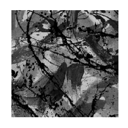
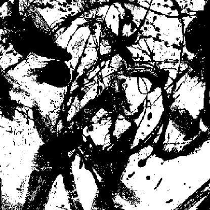
Figure 4: Sample of Les Automatiste painting and black pigment pattern (image A05).

Figure 4 shows a section of a drip painting from Les Automatistes, as well as the filtered black pigment pattern. Table 4 lists the calculated Box and information Dimensions for select works by Les Automatistes, subject to the same selection criteria as before.

As with Pollock’s drip works, the dimensions of the patterns fall roughly between $1.6-1.8$. The box and information dimensions do not explicitly differentiate between Pollock’s work and that of Les Automatistes. In fact, the difference in the average fractal dimensions for each artists was shown to be statistically insignificant using a two-way ANOVA in Reference [9]. The lighter colors display mildly lower dimensions than the darker pigments, although this may be due to cutoff limitations of the filtering process. Similar behavior was observed in the images by Pollock, so whether or not this is an actual artifact of the pattern or a numerical effect is a subject for future investigations.

While this was somewhat the case with Pollock’s works, there are perhaps sufficient discrepancies to suggest that such a measure could be indicative of different uses of colors and techniques between these artists. This includes using lighter colors for balance in an image, versus their use for adding contrasting depth.

In any event, the general equivalence of the dimensions of Pollock’s works and those of Les Automatistes suggests that the utility of this technique as a “fingerprinting” mechanism for individual artwork/artist association may be in vain. As with the galaxy clustering models, one could assert that the technique can isolate only construction method, and not structural variation within the method. Those who are dissuaded by the effective reductionist implications of the analysis may find comfort herein. In order to further address this point, the multifractal analysis will be addressed in Section 7.

7 Multifractal Spectrum of Non-Representational Images

Figure 5 shows the range of generalized dimensions $D_{q}$ for these patterns. Note that the overall depth of the generalized dimension spectrum is not excessive, suggestive that if these patterns can be described by multifractal statistics, their overall structure is not that extensive. Furthermore, note that for the majority of the cases considered, there is no appreciable difference in the range or shape of the spectrum. The errors from the linear fits are generally of the order 0.05 or less, but these may be underestimates since no error is introduced for variation in the color. The limiting values of $D_{\infty}$ give less intuitive insight into the densest clustering regions, unlike in the case of the three-dimensional sets considered earlier.

Table 5 shows inhomogeneity measure for several Pollock and Automatistes works, defined by Equation (8). In general, the results suggest that Pollock’s works tend to be “deeper” than those by the Automatistes (i.e. greater degree of inhomogeneity), perhaps a result of painting styles and refinement techniques. This could hint at a potential method of distinction for the sets of similar classes, but one must be extremely cautious of the selection criteria for the pattern in question. It is more likely that these measurements are simply too “noisy” for any useful approximation.

8 Comparison of Construction Method: Gestural Expressionism versus Artonomy

The utility of the analysis methods contained herein seem limited in the context of analysis of differing works of the abstract expressionist class. For the cases considered, the variance in the data seem too small to be of any particular import for specific identification. However, when applied to other images, certain differences do arise, enabling one to make distinctions at least on some level.

In particular, the artwork of Tsion Avital [11] will be considered. In his seminal work on the subject [11], Avital introduces the concept of Artonomy, the focal blend of artistic expressionism with scientific order. A complete description of the intricacies of the method will not be discussed here, and the interested reader is referred to the aforementioned citation for further details. The crucial point is that the construction “philosophy” for these images is strictly different than those of the gestural expressionist class considered previously.

Avital notes that the concept of Artonomy is based on certain principles of of “isotropy” in the creation process. There are no preferred sets of colors, and the use and applications of each color are deemed “equal” in value to every other. Colors (or elements) are combined into a variety of rigorously-defined mathematical sets (dubbed “moments”), and the final paintings are constructed from combinations of these moments subject to the appropriate rules. Paints are applied in a simple manner (e.g. controlled brush, or “toothbrush spray”) and as with the color selection, there is no preferred method.

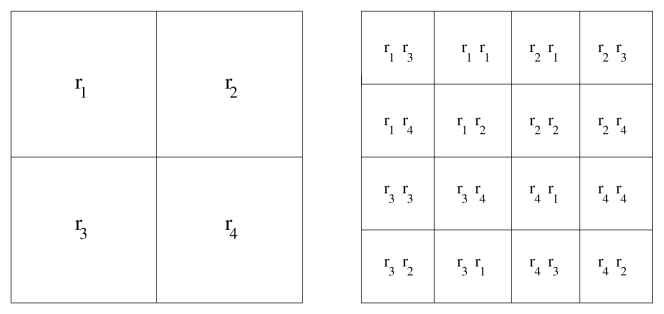
Figure 6: Multifractal scaling behavior, showing 1-level reduction of distribution with probabilities $r_{1},r_{2},r_{3},$ and $r_{4}$.

The moments are methodically positioned on the canvas in a recursive fashion quite reminiscent of the basic structure of multifractals (such as, for example, the framework outlined in Figure 6). Of particular interest is Avital’s “type $\gamma$” moment construction rule [11], which operates on the basis of information density on the canvas. Here, he defines the density as low when like colors or hues are assembled (homogeneous elements), and high with the neighboring placement of contrasting elements (heterogeneous elements). Avital defines an abstract field as one which is comprised of low density regions, and a concrete field as one composed of high density regions. Abstract and concrete fields may be inter-mixed to form heterogeneous fields. Images AV01-03 represent “homogeneous” constructs, while AV04-06 are “heterogeneous”.

So, in a sense, comparison of gestural expressionist “structures” with those of Avital constitutes a contrast in construction methodologies – random versus algorithmic – and thus Avital’s works can be taken to be a control or model comparison.

Table 6 shows measured generalized multifractal dimensions for various color distributions in Avital’s works. It is somewhat difficult to define an exact base color in the homogeneous images (AV01-03), since the resulting pattern is due to integrated “aerosol” deposition. In any event, note that unlike the Pollock and Automatistes images, Avital’s works show no significant multiscaling behavior. In many cases, the calculated $D_{\infty}$ is higher than $D_{0}$, yielding a negative $\Delta_{0,\infty}$. It should be noted that similar behavior was observed for some monofractals and simple geometric shapes (i.e. objects for which there is a single scaling dimension), where the $D_{q}$ for small $q$ tend to underestimate the actual dimension. Also, if one considers the associated statistical error, then these negative values are easily accounted for. Thus, it can be concluded that Avital’s systemic blobs are devoid of the “rich” structure with which the gestural expressionists endow their works, due perhaps in part to the very algorithmic (less random) nature of the construction.

Furthermore, Avital’s homogeneous works (e.g. AV01) were constructed from the spray of a paint from a toothbrush. Thus, the resulting structure is probably similar to the deposition from an aerosol source. The dimensionality most likely reflects this mechanism, to a certain extent. Avital’s heterogeneous works (AV11, AV12) were constructed with controlled paint brush strokes. So, these could actually be considered two separate sub-construction mechanisms.

9 Reconstructing Images From the Multifractal Spectra

Accurate determination of the multifractal spectra of singularities for a dynamical process can yield important information about its construction processes and associated constraints. As previously mentioned, the $D_{q}$ provide important information about the n-tuple “pair-wise” clustering behavior of the set, and provide a unique characterization of the object under investigation.

The quantities thus obtained can be used as physical constraints to be used in development of any model, and can perhaps yield interesting information about the dynamics of the pattern generator during the construction phase. Since the multifractal analysis herein seems only to have the ability to discern one class of structure from another, one must ask whether or not there is a useful tool to distinguish between like sets. A short analysis is performed herein on the like image arrays of the abstract expressionist class, in order to address this problem.

By definition, a multifractal is an inhomogeneous recursive scaling (a multifractal lattice). Suppose a square (or box, to be consistent with the current nomenclature) is divided into four sub-units of equal area. Then, one can describe the relative portion of the pattern contained in each box by the probabilities $r_{1},r_{2},r_{3}$, and $r_{4}$ respectively (see Figure 6).

At the next level of recursion, the weights $r_{i}$ are randomly reassigned to each sub-box of the previous layer, and the process repeats (cascades) down to any level of recursion desired.

Recall that the generalized dimensions are calculated from the partition function (5), and furthermore $(q-1)D_{q}=\tau(q)$. From (7), one can estimate the difference between two successive cut scales $\delta$ and $\delta/2$ (c.f. Figure 6) as

$$D_{q}(q-1)=\tau(q)=\frac{\Delta\log[Z(q,\delta)]}{\Delta\log[\delta]}~{},$$ (10)

In terms of the probability $r_{i}$ for each box, this becomes

$$\frac{\Delta\log[Z(q,\delta)]}{\Delta\log[\delta]}=\frac{\log[\sum_{i}r_{i}^{q}]-\log[\sum_{j}r_{j}^{q}\sum_{k}r_{k}^{q}]}{\log[\delta]-\log[\delta/2]}~{},$$ (11)

which reduces to

$$D_{q}(1-q)=\frac{\log[Z(q,\delta)]}{\log(2)}~{},$$ (12)

So, one can substitute $Z(q,\delta)=r_{1}^{q}+r_{2}^{q}+r_{3}^{q}+r_{4}^{q}$ to obtain

$$r_{1}^{q}+r_{2}^{q}+r_{3}^{q}+r_{4}^{q}=2^{D_{q}(1-q)}~{},$$ (13)

and the distribution probabilities $r_{i}$ may be obtained from a system of four equations. Note that this expression may be simplified, by noting the constraint $r_{1}+r_{2}+r_{3}+r_{4}=1$. Furthermore, the $q=2$ version of Equation 13 represents the equation of a 4-sphere, whose roots may be easily obtained.

Hence, the system of four equations may be reduced to a system of two unknowns, in this case $r_{3}$ and $r_{4}$. The values of the four possible $r_{i}$ may be isolated by optimizing the possible values of $r_{3},r_{4}$ which fit the measured $D_{q}$ spectrum of generalized dimensions. This is achieved by finding sets of $r_{i}$ for which the individual separations $\Delta D_{i}=D_{\rm calculated}-D_{\rm measured}<\epsilon$, for $\epsilon\sim 0.0001$ on average.

In Table 7, the $r_{i}$ values for various shapes of known monofractal dimension are presented. Note that for a figure of topological dimension $D_{T}=1$ (e.g. the line), the weighting factors suggest that for the appropriate cut of the plane in Figure 6, the shape will only have a nonzero probability of being in any two of the 4 sub-boxes, a result which certainly makes sense. Similarly, a figure of dimension $D_{T}=2$, which “fills the plane”, will have equal probability of being in every box. The negative component for the Koch Curve (Island) is most likely the result of numerical uncertainty, since negative probabilities would not make sense. The calculated $r_{i}$s for the Koch Curve and Sierpinski Gasket can also be interpreted to reflect the construction algorithms and symmetries for each figure.

Table 8 lists the calculated values of $r_{i}$ for the “anchor layer” pigment shapes in several of the images considered previously. The values are relatively consistent for each painting, although this is not a particularly surprising result, since the $D_{q}$ spectra themselves are not significantly different.

Each set is characterized by a rather even distribution amongst three of the boxes, and a fourth which is smaller by an order of magnitude. The almost homogeneous distribution is no doubt reflective of the fact that the generalized dimensions are close to 2. It can be shown that for a distribution with $r_{i}=0.25$ for all $i$, the generalized dimensions all collapse to 2 (or vice versa).

It may be somewhat discouraging to note that these values are rather close to one another, and are seemingly indistinguishable. However, it should be noted that the formalism outlined above is not a singular representation of a multifractal scaling process. Four quadrants have been used to show recursive scaling in part for computational efficiency. This could be a significant source of error if the scaling behavior is radically different than this model requires. Additionally, this may again be a fundamental problem with the resolution limitations of the method.

The parameters herein can conceivably be used in the formulation of a physical model which could reproduce the associated images, at least on a statistical level. Furthermore, the authors of [5] have studied video recordings of Jackson Pollock in his creative process, and have found that the “fractality” of the overall work took less than a minute to define. Surely, this provides an additional constraint on a such a cascading model.

On a subjective level, one wonders whether or not the smaller fourth quadrant could conceivably be interpreted as an imprint of the presence of the “source” of the image pattern (in this case, the physical presence of the artist). That is, at any point during the construction of the painting, the artist has free choice to paint in three of the four “quadrants” (the last being occupied by himself). Thus, this could be nested in the recursion, and detectable by such an analysis. If this explanation were to accurately represent the evolution of the pattern, it could be used to distinguish between patterns constructed by humans, and those created by machines or other natural processes.

10 Visual Multifractals

The analysis in the previous Sections relied predominantly on a color filtering process dependent on the distance in RGB space of pixel color to its target “match”. However, many reports suggest that the hierarchical clustering of the images has some variety of psychological effect on the viewer. While using RGB primaries as the filtering criteria isolated the physical structure of the blob, it may not be an effective measure of the perceived structure. Taylor et al. have recently studied physiological responses to fractal viewing, and have concluded that observers do exhibit definite responses when presented with certain fractal patterns [7, 6].

The problem of structure identification and discrimination is not a new one in psychological circles, nor is it by any means a solved one. Implicitly related to this topic, the authors of reference [31] discuss the perceptability of hierarchical structures in abstract or non-representational constructs (whose subject matter is used in a comparative study in Section 8). In fact, rapid object recognition and categorization via boundary isolation versus “blob” identification is a subject of growing scientific interest (see [32] and related references therein).

A complete understanding of the nature of color perception is still lacking. Thus, the notion of a visual fractal is introduced in contrast to those fractals previously considered. Instead of direct observation of colors, the focus is instead shifted to edge structures. This is effectively an analysis of luminance gradients within the image, and not directly on the RGB color field distribution (although the luminance values are determined by R, G, and B mixes). In fact, after completing this research, the work of references [33] was discovered. Therein, the authors discuss the potential uses of measuring the multifractal spectrum of luminance gradients in natural color images, to determine whether or not it conveys relevant information about the image. The analysis presented herein is quite similar in these respects, and thus is not performed without physical justification.

10.1 Luminance Edges as Visual Fractals

While ripe with theory, the actual dynamics of human color visual processing are poorly understood, yet it is clear that one does not require a wealth of color information to visualize a scene. A subject of ongoing interest (see e.g. [34] and similar references) is whether or not object/pattern recognition occurs on the level of “blob” or “edge” identification. Studies of eye moments in subjects viewing artistic scenes seem to support the notion that human fixate on particular aspects of an image, supporting the notion that “blobs” are viewed [35] but it is perhaps unclear as to how these objects are distinguished.

Similarly, the images formed by one’s brain may not be fully representative of the scene which one views. Both chromatic and achromatic information received from stimulation of the photopigment receptors in the rods and cones, are “preprocessed” before being sent to the visual cortex via the optic nerve.

In a similar vein, it is useful to find a “one-parameter” method of analysis for such color images, as an attempt to find a suitable way to discriminate between them. The results of the previous Sections suggest that different choice of colors yield somewhat differing dimensions, so it would be helpful to find an element common to all images which is independent of any particular color. Thus, one can consider analyzing luminance properties of the image.

Edge detection in the visual system occurs on several different levels, although it is not necessarily know which one is “dominant”. One such mechanism is known as lateral inhibition (LI). In short, this process measures the relative excitatory signal output from one photoreceptor with inhibitory signals from adjacent neighbors, effectively producing a difference output signal which is sent to the visual cortex. The result is that the strongest excitatory signals will be sent from those retinal neurons which detect luminance changes across the field [27].

Coupled to the visual system’s ability to interpolate information in a field from missing stimuli (e.g. as with the blind spot), LI can create artificial luminance and brightness variation effects which are not physically present in the original scene [27]. For example, a black and white checkerboard will seem to have greyscale variations across the pattern. The intensity (luminance) of the central squares is the same in each case, but the square surrounded by white appears to be darker than the other (see Figure 7). This exemplifies the eye’s ability to create artificial variations in scenes which are otherwise not physically present. Hence, this provides a rather simple example of how visual interpretation of an object may not be complete commensurate with the actual physical characteristics.

Lateral inhibition is, however, only one of several mechanisms responsible for the detection of contrast edges in a visual field. While LI mechanisms operate in the eye, such detection is known to occur in the visual cortex itself. Hubel and Wiesel were responsible for the discovery of “orientation columns” within the visual cortex, cells responsible for the identification of specific edges or boundaries orientations. The aforementioned researchers share the 1981 Nobel Prize in Medicine for their research efforts. The interested reader is directed to reference [36] for an expository account of their work. Thus, there is sufficient physiological and psychological motivation to consider possible structural differences in contrast edges.

The transformation from RGB primaries is of the form $Y=0.299\;R+0.587\;G+0.114\;B$ [37] (note that the color coordinates must be normalized), which implies pure white coordinates $(R,G,B)=(1.0,1.0,1.0)$. Note the relatively higher weighting of R and G primaries to B. This is reflective of the eye’s sensitivity to similar wavelength intensities. In fact, these roughly correspond to the three basic types of cone cells with similar thresholds, denoted as L, M, and S (for long, medium, and short wavelengths). This is actually one component of a separate CIE color system known as YIQ (the channels I and Q are encode chromacy information, hue and saturation). The luminance channel is what one generally associates with greyscale images, an in fact is that information which is transmitted in black and white television signals [37]. Edge detection is performed by generally-available image manipulation tools, which measure the vector sum of two perpendicular Sobel gradient operators (see e.g. [38] for more information).

These are perhaps crude approximations to the actual physiological processes at hand, so implicit limitations in the estimates should be accordingly recognized. Certainly, the method does not purport to be a realistic model of the visual system. It should, however, provide a decent first-pass approximation to any inherent structures and effects therein.

10.2 Pollock vs Les Automatistes

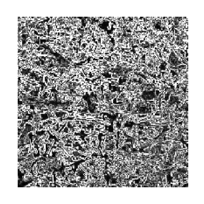
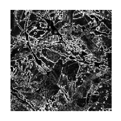
Figure 8: Sample luminance gradients for P02 (left) and A05 (right).

Figure 8 shows a sample edge-detect transform for a images of Pollock and Les Automatistes, with the associated $D_{q}$ spectra in Figure 9. For the color-filter process, the target color in this case is pure white, and the color radius is taken to be the linear distance away from the point. Thus, for a small radius, the images with the highest gradients will have the largest dimensions. Table 9 and 10 give dimensions for both $\beta=1$ and $\beta=30$, which give an indication of the “value” of the strongest gradients. It should be noted that since neuronal firings are triggered by threshold-breaking stimuli, a discrete cutoff is more realistic than a Gaussian drop-off.

The calculated box dimensions for the edge-detected Pollock images tend to be higher than for the individual blobs, generally $D_{0}>1.8$. This can be interpreted as implying that the luminance edges form a much more complex visual field, and that the edge lines are more “space filling”, and providing a “busier” or “fuller” visual experience.

When the method is applied to the gestural expressionist works of Les Automatistes, differences become more apparent (see Figure 9). The box dimensions for Les Automatistes is generally lower (albeit not much) than those of Pollock’s. Similar results are obtained for other images (see Table 9). Note that the measured dimensions do not increase significantly from $\beta=1$ to $\beta=30$.

This suggests that there is a potential visual difference between images by these different artists. While the final products may resemble each other at first glance, the intricacies of the two images from a luminance gradient / visual standpoint appear quite different. Again, in Reference [9] the difference in average fractal dimension of the “edge” patterns was determined to be statistically significant.

Based on the work of previous authors [39] and their own survey on preferential response to drip patterns, the authors of [5] conclude that patterns possessing a fractal dimension of roughly 1.8 are inherently aesthetically-pleasing to the observer. A follow-up study suggests that “creative individuals” have a preference for high values of $D$ [40]. One could imagine that this type of perceived structural difference could contribute to an observer’s “appreciation” of one image or style over another.

10.3 Comparison With Avital

Avital’s definitions of homogeneous and heterogeneous fields (not to be confused with homogeneous fractal distributions), along with the concept of information content, are a natural extension of the notions of luminance gradient structures proposed in Section 10.1. In fact, the very notion of information content is at the heart of the multifractal formalism. Thus, a luminance-gradient analysis of Avital’s images should reveal certain properties about the formulaic construction of the pieces, or at the very least lend contrast to the more psychological algorithms used by the Abstract Expressionist artists (or perhaps any other artist).

Table 10 shows the effective edge-detection dimensions of various works by Avital [11], as well as a rough definition of the type of image. Figure 9 shows the associated spectra, in comparison to the previous images. Since reproduction of every image in this work is not warranted, The previous color panels demonstrate the general qualities of each type of image (labeled homogeneous and heterogeneous), while Figure 10 shows the resulting luminance gradients. It should be noted that the images classified as “homogeneous” all conform to Avital’s “S/D/$\delta$” construction algorithm (made from the spray of a toothbrush) [11], which indeed embodies an inherently smooth transition to complexity vis-a-vis color selection and application. In contrast, the images noted as “heterogeneous” are from Avital’s “S/C/$\gamma$” algorithm, which allows for a counterbalance between abstractness and concreteness. These are simply painted with controlled brush strokes.

The lower dimensions and higher error for the homogeneous images in Table 10 demonstrate the low color contrast nature of the images, and hence the shallow depth of luminance variation across the canvas. In particular, note that while image AV01 is physically a mix of bright pigments, there is virtually no strong luminance gradient across the canvas (hence to effective dimension of 0). These dimensions imply there is little “luminance information” in the fields. As the images begin to approach heterogeneity, the background field is contrasted with patches of color, whose overall boundaries are quite regular. This is indicative by the relatively low range of $D_{0}=1.1-1.3$, in contrast to the exceedingly high dimensionality of the gestural expressionist paintings, as seen in Table 9. The latter is indicative that the luminance gradients densely fill the canvas for this particular school or movement, while Avital’s shapes are more concentrated and simple.

Thus, Avital’s homogeneous work is less “interesting” from an edge detect view than the Pollock or Les Automatistes images considered (there is less edge information conveyed about the scene), while the heterogeneous work brings focus to particular objects via these edges (although still with much lower dimension that the gestural expressionist images).

These results suggest that this analysis method could distinguish between sources, as well as construction mechanisms of the images. Further investigation would be required. However, whether or not this type of distinction is possible, identification of such structural signatures could have applications in external fields. For example, albeit beyond the scope of physics, visual detection of fractal structure in luminance gradients could have profound consequences for the fields of aesthetics and visual appreciation of complex scenes (e.g. what qualities makes an image interesting to us?).

It is interesting to note that Avital himself classified works such as Pollock’s as “moment type $\omega$”, whose paradigm rests on the notion of “arbitrariness”, in which the combinations of elements (moments) are scattered at personal will about the canvas (he further notes these to require “minimal capacity of inventiveness”, and casts Pollock’s art as containing nothing meaningful or interesting [11]). Avital is careful to note the distinction between “arbitrariness” (whose choice of elements is human) and “randomness” (whose source is instead probabilistic). Unfortunately, Avital presents no simulations of type-$\omega$, so it is not possible to compare these with the works of the gestural expressionists considered previously.

11 Potential Limitations of the Method

Of course, the method described herein is not without limitations, and is only designed to be a “first-order” attack of the issues at hand. As discussed previously, digital image analysis techniques provide a statistical description of the entire physical image, with no regard for perceptual interpretations by observers. The calculated dimensions assumed equal weighting for all portions of the canvas, when in fact (depending on the distance from which they view the scene) observers will not register all portions of the field equally. Both rod and cone cells are unevenly distributed about the retina, with a disproportionately large number of cones clustered in the fovea centralis [27]. This cone clustering is crucial for perception of color and fine visual detail via fixation, and is the primary reason for the drop in acuity in peripheral vision.

So, if the image of interest fills the visual field, only the central-most regions will convey the largest amount of information. However, this should not necessarily affect the overall “visual estimation” of the fractal nature of the piece, although edges may become more blurred (resulting in potential shifts in a “visual multifractal spectrum”). Furthermore, the method does not account for other biasing effects such as color blindness, or any visual acuity drops (e.g. myopia or other focal abnormalities). The robustness tests of Section 5 suggest that the dimensionality of patterns will increase for dispersive patterns (as they should, approaching homogeneity), which could replicate such vision problems.

Finally, the methods outlined herein do not all complete correspond to actual physiological processes which occur in the eye. Reference [27] provides several alternative color space transformations which are perhaps more appropriate for the actual analysis of cone/photoreceptor excitations from lightness/luminance and chromatic stimuli. A full investigation and implementation of these methods is discussed in Reference [28].

12 Concluding Remarks and Future Directions

The use of fractal and multifractal analysis as a discriminator or fingerprint method for classifying abstract expressionist art is a budding field. However, the available results are indicative that the method may well yield promising results. The fractal signatures obtained from paint blobs are not significantly different from one another, implying that this method is not useful for “authenticating” works by any one particular artist within a movement. It apparently does differentiate between the movements themselves. This is similar to the behavior observed in [10], where the multifractal spectrum was shown to differentiate between galaxy cluster formation mechanisms, but could not discriminate between instances within the same model. The “edge multifractal” does yield differentiable results, curiously, which based on aspects of visual processing lends to the interpretation that this could represent some type of “aesthetic preference”.

One of the motivational questions which inspired the fractal analysis of gestural expressionist art is: “Does there exist an inherent structure within the painted patterns which one perceives, and hence yields an unconscious psychological effect on the observer?”. Rephrased, on can pose the question: does the brain possess a mechanism whereby the observer can gain information from a scene previously unknown to them?

This question certainly addresses the very heart of recognition and learning methodologies, but unfortunately the exact neural mechanisms which lead to cognition are not well understood. Recent discoveries in Neuroscience have paved the way for a potential revolution in this field, however.

Recent studies have revealed striking neural activity in several species of primates which respond not only to physical imitation of observed movements by others, but also passive observation of such actions. That is, such neural firings are indicative that the individual need not repeat the action in order to cognitively process its meaning – quite literally, a case of “monkey-see, monkey-do”. Based on these imitation characteristics, such cells have been dubbed mirror neurons. For a basic introduction, see [41] and references therein.

Additional studies suggest that mirror neurons may be present in higher species of primates (and in particular may be central to the development of language skills in humans [42]). If observation of action can trigger their firings and initiate comprehension of its meaning, then it may not be unreasonable to expect that observation of the trace of an action can also prompt similar neurophysiological responses.

The authors of [5] note that many natural patterns possess multifractal scaling behavior, but these are not “art” per se. What is the underlying differentiator, then, that ascribes to these statistically-similar patterns the label of “art”? Thus, by observing a complex but statistically-ordered scene such as Pollock’s art, mirror neurons could help to bridge the gap between the initial visual processing and associative comprehension and appreciation of the actions required to form the work [43]. Further study into these hypotheses are currently underway.

Acknowledgments
We gratefully thank Tsion Avital for permission to reproduce his art. This work made possible by grants from the Natural Sciences and Engineering Council of Canada (NSERC) and by financial support from the Walter C. Sumner foundation.

ID	Title (Date)	Dimensions (cm2)
P01	Blue Poles (1952)	486.8 $\times$ 210
P02	Autumn Rhythm (1950)	525.8 $\times$ 266.7
P03	Lavender Mist (1950)	300 $\times$ 221
P04	Reflections of the Big Dipper (1947)	111 $\times$ 92.1
P05	Number One A 1948	$172.7\times$ 264.2
P06	Number One 1949	160 $\times$ 259
A01	Au chateau d’Argol (1947)	55 $\times$ 50.5
A02	Fièvres (1976)	65 $\times$ 80
A03	Tumulte (1973)	81 $\times$ 101.5
A04	Voyage au bout du vent (1978)	137 $\times$ 188
A05	Suite marocaine no. 1 (1975)	81.3 $\times$ 101
A06	La danse et l’espoir (1975)	81.5 $\times$ 101
A07	Sans titre, Montréal (1959)	56 $\times$ 43

Table 1: Catalog of Jackson Pollock (P01-06) and Les Automatistes (A01-07) images used in analysis.

Fit	$\beta=$ 10	20	30
P01 (black)
$D_{0}$	1.51 (0.05)	1.68 (0.03)	1.72 (0.03)
$D_{1}$	1.46 (0.02)	1.63 (0.02)	1.67 (0.02)
P01 (red)
$D_{0}$	1.33 (0.07)	1.54 (0.05)	1.64 (0.04)
$D_{1}$	1.22 (0.03)	1.42 (0.02)	1.54 (0.02)
P02 (black)
$D_{0}$	1.66 (0.03)	1.70 (0.03)	1.72 (0.03)
$D_{1}$	1.66 (0.02)	1.70 (0.02)	1.72 (0.02)
P03 (black)
$D_{0}$	1.73 (0.06)	1.80 (0.05)	1.84 (0.04)
$D_{1}$	1.64 (0.05)	1.72 (0.04)	1.76 (0.03)
P04 (black)
$D_{0}$	1.70 (0.05)	1.77 (0.04)	1.81 (0.04)
$D_{1}$	1.67 (0.03)	1.73 (0.03)	1.77 (0.03)
P05 (black)
$D_{0}$	1.72 (0.04)	1.77 (0.04)	1.80 (0.03)
$D_{1}$	1.65 (0.03)	1.70 (0.02)	1.74 (0.02)
P06 (blue-grey)
$D_{0}$	1.64 (0.06)	1.73 (0.05)	1.78 (0.04)
$D_{1}$	1.60 (0.05)	1.68 (0.04)	1.73 (0.03)
P06 (cream)
$D_{0}$	1.52 (0.10)	1.71 (0.06)	1.76 (0.04)
$D_{1}$	1.49 (0.08)	1.65 (0.05)	1.70 (0.04)

Table 2: Box ($D_{0}$) and information ($D_{1}$) estimates for select Jackson Pollock paintings.

Painting	$\beta$ = 5	10	20
Blue Poles	1.70 (0.03)	1.72 (0.02)	1.75 (0.02)
	1.65 (0.02)	1.67 (0.02)	1.71 (0.02)
Reflections	1.81 (0.03)	1.84 (0.03)	1.87 (0.02)
	1.76 (0.02)	1.79 (0.01)	1.84 (0.01)
Number One 1949	1.76 (0.04)	1.79 (0.03)	1.82 (0.03)
	1.72 (0.02)	1.75 (0.02)	1.80 (0.01)

Table 3: $D_{B}$ (top row) and $D_{I}$ (bottom row) measurements for random pixel displacements of 5, 10, and 20 pixels. Error (in brackets) is that of the least-squares fit.

Image	$D_{0}$	$D_{1}$
A01 (black)	1.92 (0.01)	1.88 (0.01)
A02 (black)	1.66 (0.05)	1.61 (0.03)
A02 (blue)	1.67 (0.07)	1.60 (0.01)
A03 (black)	1.69 (0.03)	1.66 (0.01)
A03 (blue)	1.61 (0.06)	1.56 (0.04)
A04 (black)	1.57 (0.07)	1.54 (0.05)
A04 (blue)	1.61 (0.07)	1.53 (0.04)
A05 (black)	1.63 (0.03)	1.61 (0.02)
A05 (green)	1.57 (0.05)	1.47 (0.02)
A06 (black)	1.73 (0.05)	1.65 (0.02)

Table 4: $D_{0}$ and $D_{1}$ for various Les Automatistes images, $\beta=20$.

Painting	$D_{0}$	$D_{\infty}$	$\Delta D_{0,\infty}$
P01	1.68 (0.03)	1.45 (0.05)	0.23 (0.06)
P02	1.70 (0.03)	1.54 (0.04)	0.16 (0.05)
P03	1.80 (0.05)	1.47 (0.03)	0.33 (0.06)
P04	1.77 (0.04)	1.60 (0.04)	0.17 (0.06)
P05	1.77 (0.03)	1.55 (0.05)	0.22 (0.06)
A01	1.92 (0.01)	1.85 (0.03)	0.07 (0.03)
A02	1.66 (0.05)	1.53 (0.05)	0.13 (0.07)
A03	1.68 (0.03)	1.62 (0.05)	0.06 (0.06)
A04	1.57 (0.07)	1.34 (0.05)	0.13 (0.09)
A05	1.63 (0.03)	1.60 (0.07)	0.03 (0.08)

Table 5: Inhomogeneity measure $\Delta D_{0,\infty}=D_{0}-D_{\infty}$ comparison between Jackson Pollock paintings and Les Automatistes works for anchor layers ($\beta=20$).

Painting	$D_{0}$	$D_{\infty}$	$\Delta_{0,\infty}$	Color
AV01 (XI)	1.56 (0.03)	1.51 (0.08)	0.05 (0.09)	Grey-green
AV02 (XIII)	1.68 (0.03)	1.71 (0.05)	-0.03 (0.06)	Yellow
AV03 (XV)	1.61 (0.02)	1.60 (0.09)	0.01 (0.09)	Blue
AV04 (III)	1.45 (0.03)	1.38 (0.07)	0.07 (0.08)	Red
AV05 (VII)	1.71 (0.02)	1.82 (0.07)	-0.09 (0.07)	Black
AV06 (VIII)	1.57 (0.04)	1.43 (0.09)	0.14 (0.10)	Yellow

Table 6: Generalized dimensions for selected Avital images. Image sources are identified by Plate number from [11].

Shape	$D_{F}$	$r_{1}$	$r_{2}$	$r_{3}$	$r_{4}$
Line	1.00	0.00	0.50	0.00	0.50
Plane	2.00	0.25	0.25	0.25	0.25
Koch Island	1.26	-0.05	0.44	0.18	0.43
Sierpinski Gasket	1.57	0.00	0.34	0.32	0.34

Table 7: Distribution probabilities $r_{i}$ for various Euclidean shapes and geometric fractals.

Painting	$p_{1}$	$p_{2}$	$p_{3}$	$p_{4}$
P01	0.03	0.27	0.30	0.40
P02	0.04	0.32	0.32	0.32
P04	0.06	0.32	0.29	0.33
P05	0.03	0.34	0.29	0.34
P06	0.03	0.30	0.29	0.38
A01	0.12	0.30	0.29	0.29
A02	0.02	0.38	0.26	0.34
A03	0.03	0.33	0.32	0.32
A04	0.01	0.41	0.36	0.22
A05	0.01	0.33	0.33	0.33

Table 8: Select distribution probabilities $r_{i}$ for various Jackson Pollock and Les Automatistes works (anchor layers).

Painting	$D_{0}(\beta=1)$	$\beta=30$
P01	1.76 (0.03)	1.78 (0.03)
P02	1.90 (0.02)	1.90 (0.02)
P04	1.89 (0.02)	1.90 (0.01)
P05	1.81 (0.04)	1.84 (0.02)
P06	1.85 (0.03)	1.87 (0.02)
A02	1.54 (0.09)	1.55 (0.05)
A03	1.67 (0.05)	1.72 (0.04)
A04	1.67 (0.05)	1.71 (0.04)
A06	1.56 (0.07)	1.64 (0.06)
A07	1.75 (0.06)	1.80 (0.04)

Table 9: Edge dimensions for selected Pollock (top) and Automatistes (bottom) images, showing higher complexity of luminance gradient patterns for greyscale distance $\beta=1,30$.

Painting	$D_{0}(\beta=1)$	$\beta=30$	Type
AV01 (XI)	0.00 (0.00)	0.00 (0.00)	Homogeneous
AV02 (XIII)	0.00 (0.00)	0.00 (0.00)	Homogeneous
AV03 (XV)	0.00 (0.00)	0.08 (0.05)	Homogeneous
AV04 (III)	0.68 (0.03)	0.83 (0.04)	Heterogeneous
AV05 (VII)	0.95 (0.05)	1.04 (0.05)	Heterogeneous
AV06 (VIII)	1.28 (0.03)	1.37 (0.04)	Heterogeneous

Table 10: Effective edge dimensions for selected Avital images for greyscale distance $\beta=1,30$. Image sources are identified by Plate number from [11].

Figure 5: Multifractal dimension spectra for select images of Table 1. Erro r bars are suppressed for easy viewing.

Figure 7: Black and white checkerboard pattern (“Hermann Grid”) showing visual luminance structure variation due to edge enhancement effects in the visual processing system.

Figure 9: $D_{q}$ spectra for luminance gradients of Pollock, Automatistes, and Avital images $(\beta=1)$. The structures are clearly separated by $D_{0}$ values, although the overall structure of the curve is similar.

Figure 10: Sample luminance gradients of images for AV01 (top) and AV06 (bottom).

References

- [1] Gliden. D. L., Schmuckler, M. A., and Clayton, K., Psych. Rev. 100, 460 (1993)
- [2] Schmuckler, M. A., and Gliden. D. L., J. Exper. Psych.: Hum. Percep. Perf. 19, 641 (1993)
- [3] Gliden, D. L., “1/f Noise in the Fundamental Forms of Psychology”, UT Austin Preprint
- [4] Taylor, R. P., Micolich, A. P., and Jonas, D., Physics World (October 1999); Nature 399 (3 June 1999); “Splashdown”, New Scientist (25 July 1998);
- [5] Taylor, R. P., Micolich, A. P., and Jonas, D., J. Conscious. Stud. 7, 137 (2000)
- [6] Spehar, B. et al., Chaos and Graphics 27 813 (2003)
- [7] Taylor, R. P. et al., J. Non-lin. Dyn. Psych. and Life Sci. 9 89 (2005)
- [8] Mureika, J. R., Topics in Multifractal Analysis of Two- and Three-Dimensional Structures in Spaces of Constant Curvature, Doctoral Thesis, University of Toronto Graduate Department of Physics (2001)
- [9] Mureika, J. R., Cupchik, G. C., and Dyer, C. C., Leonardo 37 (1), 53–56 (2004)
- [10] Mureika, J. R. and Dyer, C. C., Gen. Rel. Grav. 36 (1), 151–184 (2004)
- [11] Avital, T., Artonomy: Systematic Art, unpublished doctoral thesis (1974)
- [12] Mandelbrot, B. B. The Fractal Geometry of Nature, W. H. Freeman and co. (1983)
- [13] Falconer, K., Fractal Geometry: Mathematical Foundations and Applications, John Wiley and Sons (1995)
- [14] Barnsley, Michael F., Fractals Everywhere (2nd ed.), Academic Press Professional (1993)
- [15] van der Lubbe, J. C., Information Theory, Cambridge University Press (1997)
- [16] Grassberger, P. and Procaccia, I., Physica 9D, 189 (1983)
- [17] Hentschel, H. G. E., and Procaccia, I., Physica 8D, 435 (1983)
- [18] Grassberger, P., Phys. Lett. 107A, 101 (1985)
- [19] Halsey, T. C. et al., Phys. Rev. A33, 1141 (1986)
- [20] Jensen, M. H., kadanoff, L. P., Procaccia, I., Phys. Rev. A36, 1409 (1987)
- [21] Tél, T., Z. Naturforsch. 43a, 1154 (1988)
- [22] Paladin, G. and Vulpiani, A., Phys. Rep. 156, no. 4, 147 (1987)
- [23] Vicsek, T., Fractal Growth Phenomena, World Scientific Press, Singapore (1989)
- [24] Robertson, Bryan, Jackson Pollock, Thames and Hudson Ltd. (1968)
- [25] Spring, J., The Essential Jackson Pollock, Andrews McMeel Publishing (1998)
- [26] Gagnon, C. and Gauthier, N. Marcel Babeau: Fugato, Imprimerie Laurentienne, Montréal (1990)
- [27] Kaiser, Peter K., and Boynton, Robert M., Human Color Vision (Second Edition), Optical Society of America (1996)
- [28] Mureika, J. R., “Fractal Dimensions in Perceptual Color Space: A Comparison Study Using Jackson Pollock’s Art”, submitted to Chaos (2005)
- [29] Kaye, b. H., A Random Walk Through Fractal Dimensions, VCH Publishers (1989)
- [30] Pastor-Satorras, R. and Riedi, R. H., J. Phys. A29, L391 (1996)
- [31] Avital, T., and Cupchik, G. C., Empirical Studies of the Arts 16, 59 (1998)
- [32] Schyns, P. G., and Oliva, A., Psych. Sci. 5 (4), 195 (1994)
- [33] Turiel, A. et al., Phys. Rev. Lett. 80, 1098 (1998); Turiel, A. et al., Phys. Rev. E 62, 1138 (2000); Turiel, A. et al., Phys. Rev. Lett. 85, 3325 (2000)
- [34] Aude, O., and Schyns, P. G., Cog. Psych. 41, 176 (2000)
- [35] Yarbus, A. L., Eye Movements and Vision, Plenum Press (1967)
- [36] Hubel, D. H., Sci. Amer. 209, 54 (1963); Hubel, D. H. and Wiesel, T. N., Sci. Amer. (September, 1979)
- [37] Foley, J., van Dam, A., Feiner, S., and Hughes, J., Computer Graphics: Principles and Practice (second edition in C), Addison-Wesley Publishing Co. (1996)
- [38] Gonzalez, R. C., and Wintz, P., Digital Image Processing (2nd ed.), Addison-Wesley Publishing Co. (1987)
- [39] Pickover, C A., Keys to Infinity, Wiley Press (1995)
- [40] Aks, D. J. and Sprott, J. C., Empirical Studies of the Arts 14, 1 (1996)
- [41] Arbib, M.A., “The mirror system hypothesis for the language-ready brain”, in Computational Approaches to the Evolution of Language and Communication, Cangelosi, A. and Parisi, D. (eds.), Berlin: Springer Verlag (2001); also “The mirror system, imitation and the evolution of language”, in Imitation in Animals and Artifacts, Nehaniv, C. and Dautenhahn, K. (eds.), Cambridge, MA: MIT Press (2002)
- [42] Rizzolatti, G. and Arbib, M. A., Trends Neurosci. 21, 188 (1998)
- [43] Arbib, M. A., personal communication