Microsolvation of Li⁺ in small He Clusters. Li⁺He_n species from Classical and Quantum Calculations

Abstract

A structural study of the smaller Li⁺He_n clusters with $n\leq 30$ has been carried out using different theoretical methods. The structures and the energetics of the clusters have been obtained using both classical energy minimization methods and quantum Diffusion Monte Carlo. The total interaction acting within the clusters has been obtained as a sum of pairwise potentials: Li⁺-He and He-He. This approximation had been shown in our earlier study 8 to give substantially correct results for energies and geometries once compared to full ab-initio calculations. The general features of the spatial structures, and their energetics, are discussed in details for the clusters up to $n=30$ and the first solvation shell is shown to be essentially completed by the first ten helium atoms.

I Introduction

The study of the nanoscopic forces which act within small aggregates of weakly interacting particles, especially within assemblies containing helium atoms, has received a great deal of attention in the last few years 1 ; 2 ; 3 because of the broad range of phenomena that can be probed under the very special conditions provided by the He nanodroplets as containers of atoms or molecules. They are indeed, ultracold homogeneous matrices where the corresponding spectra often reach very high resolution due to the superfluid properties of the helium droplet 4 .

The possibility of causing electronic excitation and/or ionization of the dopant species can offer additional ways of probing the modified interaction between the new ionic species and the gentle matrix of the helium droplets 3 since the ensuing distribution surrounding the molecular impurity is usually markedly deformed as a consequence of the electrostriction effects on the solvent brought on by the induction forces between the charged dopant and the helium atoms in the droplet 5a ; 5 . The analysis of such effects in the case of lithium-containing impurities has been particularly intriguing because of the expected simplicity of the electronic structures involved and, at the same time, the unusual bonding behaviour of such systems. Furthermore, experiments in which the droplet was ionized after capture of Li atoms 7 have revealed a wealth of newly formed species like Li⁺, Li${}^{+}_{2}$ and LiHe⁺ which are produced during droplet fragmentation and evaporation thereby triggering the corresponding analysis of structure and bonding behaviour from theory and computations.

In a previous computational investigation 8 on the interaction of Li⁺ with $n$ helium atoms, with $n$ varying from 1 to 6, we have shown, in fact, that the energy optimized structures of the clusters were largely determined by two-body (2B) forces, with the many-body effects being fairly negligible for determining the final geometry of those small aggregates. In the present study we have therefore decided to analyze in greater detail the quantum states and binding energies of the larger structures of Li⁺ impurities within the helium droplets in order to extend our computational knowledge on such species.

The next Section briefly describes the LiHe⁺ Potential Energy Curve (PEC) used here. The results for the trimer ground state are given and discussed in Section III, where we report the features obtained using the distributed Gaussian functions (DGF) method 11 ; 12 ; 13 ; 14 and the quantum Diffusion Monte Carlo (DMC) method 9 , in comparison with the values obtained via a classical minimization procedure. Section IV extends the discussion to the larger species, whose energetics and structural features, both obtained with DMC and classical methods, are analyzed.

II The pairwise potentials

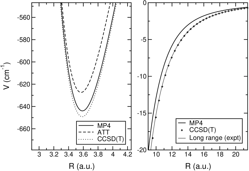
Figure 1: Left panel: comparison of different calculations of the well region Solid line: results from Ref. 8 ; dashes from ref. 17 (ATT); dots from Ref. 19 (CCSD(T)). Right panel: comparison of the long-range polarization potential (thin line) with the long range behavior of two of the computed PEC’s.

The actual potential energy curve (PEC) for Li⁺He has been studied before because of its interest in modeling low-energy plasmas 16 . Alrich and coworkers suggested earlier on a model potential as a variant of the Tang-Toennies model 17 while recent calculations of Soldán et al. 19 employed a CCSD(T) treatment and used the aug-cc-pV5Z basis set. Recently, we have also carried out a new set of calculations on these clusters 8 using the MP4 method and the cc-pV-5Z basis set. The results from the ab initio calculation of Ref. 19 , the potential obtained from a MP4/cc-pV-5Z calculation and the model potential of Ref. 17 are presented in pictorial form by the two panels of Fig. 1 where in the left panel we show the region of the potential minimum. One clearly sees there that the deepest well is presented by the CCSD(T) calculations of 19 , while the model potential of 17 has the most shallow well. The corresponding long-range part of the PEC’s is reported on the right-hand side panel, where one can see that the calculations of 19 closely follow the long-range dipole polarisability tail, computed here with $\alpha_{He}$=1.3832 $a_{0}^{3}$ 20 . In Table 1 we report the bound states of the Li⁺-He diatom when $J=0$ for the three different potentials calculated using a DVR scheme dvr using 2000 grid points in the interval 1.5, 200 a.u.. In the case of the potential of Murrel et al. 19 our results are almost coincident with those provided by the same authors. As can be seen there, the three potentials yield rather similar energies, although in the well region the agreement is better between those from the MP4 potential and those from Soldan et al.. On the other hand, the latter has a long range behavior very similar to that from the semi-empirical ATT potential (see also Fig. 1 where we compare it to the “experimental” long range behavior): both these potentials, indeed, support 8 bound states while the potential calculated by us with MP4 8 yields only 7 bound states for $J=0$. The MP4 potential therefore seems not to provide a good description of the long range, inductive tail because of the lack of augmented atomic functions in the basis set from which it has been obtained. Hence, we have decided to employ in the following the CCSD(T) PEC from Soldan et al..

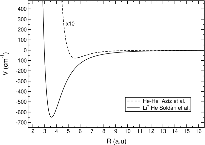
Figure 2: Comparison of the LiHe⁺ potential from Ref. 19 and the He-He one from Ref. 24 . The He-He potential has been multiplied by ten.

For the He₂ dimer we have employed the semiempirical potential (LM2M2) of Aziz and Slaman 24 : in Fig. 2 we sketch the two pair potentials used in our calculations. The two potentials are completely different: the Li⁺-He one is dominated by electrostatic and induction forces while the He-He interaction is much weaker and purely van der Waals in nature.

As we mentioned above, the full interaction that acts in the M⁺Rg_n clusters can be approximated by a sum of pairwise potentials. The main source of error in this model is due to the absence of the repulsive interactions between the induced dipoles on the helium atoms, especially those that are located near the ionic center. These interactions, however, can be taken to be very small for rare gas atoms and especially for helium partners. For example, in Ref. 29 for the analogous situation of the anionic dopant Cl^- in Ar clusters it has been shown that the inclusion of the leading terms of such 3-body forces does not alter substantially the energetics and the structure of the clusters: in ref. 8 we have discussed and confirmed this feature for the system analyzed here. Furthermore, since the charge delocalization in Li⁺-He_n is very small 28 and the interaction is mostly determined by ¨physical¨ forces (charge/induced multipole) rather than by ¨chemical¨ effects, all the helium atoms that are attached directly to the ionic center can be considered to be equivalent because there is no detectable tendency for the latter to preferentially form chemically bound structures with only a subset of such adatoms, a fact which would therefore differentiate some of the binding effects with respect to those in the rest of the cluster.

III An outline of the computational tools

III.1 The classical optimization

The total potential in each cluster is described by the sum of pairwise potentials and searching for the global minimum in this hypersurface $V_{TOT}$ will give us the lowest energy structure for each aggregate from a classical picture viewpoint. All the classical minimizations were carried out with a modified version of the OPTIM code by Wales wales94 . This code is based on the eigenvector following method. The basis of this method is the introduction of an additional Lagrange parameter into a “traditional” optimization framework baker86 , which seeks to simultaneously minimize in all directions. All searches were conducted in Cartesian coordinates using projection operators to remove overall translation and rotation following Baker and Hehre baker91 . Analytic first and second derivatives of the energy were employed at every step, and the resulting stationary point energies and geometries are essentially exact for the model potential in question. The details of the method as applied in our group have been given before and therefore will not be repeated here.

III.2 The quantum stochastic calculation (DMC)

The Diffusion MonteCarlo Method has been extensively discussed in a number of papers (Refs. hammond ; ceperley ; suhm and references therein) and therefore will not be repeated here.

In our implementation a random walk technique is used to solve the diffusion equation where a large number of random walkers is propagated with time steps $\Delta\tau$ starting from an arbitrarily chosen initial distribution. The ground state energy $E_{0}$ is obtained by averaging $E_{L}(\mathbf{r})$ over the final mixed distributions $f(\mathbf{r},t)=\psi_{T}(\mathbf{r},t)\psi(\mathbf{r},t)$:

$$<E_{L}>=\frac{\int E_{L}(\mathbf{r})f(\mathbf{r},\tau_{f})d\mathbf{r}}{\int f(\mathbf{r},\tau_{f})d\mathbf{r}}=\frac{\int\psi_{0}(\mathbf{r})\hat{H}\psi_{T}(\mathbf{r})d\mathbf{r}}{\int\psi_{0}(\mathbf{r})\psi_{T}(\mathbf{r})d\mathbf{r}}=E_{0}$$ (1)

The energy is therefore affected by a bias due to the use of a mixed distribution. The bias is however minimized by using very long propagation time and very short timesteps. Expectation values of position operators $\hat{A}(\mathbf{r})$ are also given by averaging over $f(\mathbf{r})$, a procedure that leads to biased distributions. However, we believe that the bias does not modify the qualitative picture of the present calculations especially because whenever our spatial distributions are compared with those from other quantum calculations (where possible) and with classically minimized structures, they are found to be in remarkable agreement with each other as we shall discuss further below.

The trial function used here for the $\mathrm{He-He}$ pairs is a product of trial wavefunction:

$$\Psi_{T}=\prod_{i,j\in\mathrm{He}}\exp\left(-\frac{p_{5}}{R_{ij}^{5}}-\frac{p_{2}}{R_{ij}^{3}}-p_{0}\log R_{ij}-p_{1}R_{ij}\right)$$ (2)

where the values of the coefficients have been taken by Ref lewerenz97 . The trial function for the $\mathrm{Li^{+}-He}$ pair has been chosen as a gaussian function centered around the energy minimum of the relative interaction. However, in order to adjust each trial wavefunction to the size of the larger clusters, its parameters have been chosen so that they make it increasingly more delocalized as the number of adatoms is increased. All prameters are available from direct requests to the corresponding author.

III.3 The distributed Gaussian Functions (DGF) expansion

The DGF method 11 ; 12 is a variational approach which solves the trimer bound state problem written in terms of the atom-atom coordinates by employing a large set of distributed Gaussian functions as a basis set.

First of all, the Hamiltonian for a triatomic system is expressed in terms of atom pair coordinates R₁, R₂ and R₃, i.e. in terms of the distances between each pair of atoms along which the Gaussian functions are distributed (see 13 for the expression of the Hamiltonian for a triatomic system with an impurity).

The total potential for the trimer is assumed to be the sum of the three two-Body potentials as discussed previously and the calculations are carried out for a zero total angular momentum. The total wavefunction for the v-th vibrational states is then expanded in terms of symmetrized basis functions

$$\Phi_{v}(R_{1},R_{2},R_{3})=\sum_{j}a_{j}^{(v)}\phi_{j}(R_{1},R_{2},R_{3})$$ (3)

with

$$\phi_{j}(R_{1},R_{2},R_{3})=N_{lmn}^{-1/2}\sum_{P\in S_{2}}P[\varphi_{l}(R_{1})\varphi_{m}(R_{2})]\varphi_{n}(R_{3})$$ (4)

for the two-identical-particle system. Here, $j$ denotes a collective index such as $j=(l\leq m;n)$ and N_lmn is a normalization constant expressed in term of the overlap integrals s${}_{pq}=\langle\varphi_{p}|\varphi_{q}\rangle$. Each one-dimensional function $\varphi_{p}$ is chosen to be a DGF (light86 ) centered at the $R_{p}$ position

$$\varphi_{p}(R_{i})=\root 4 \of{2A_{p}\over\pi}e^{-A_{p}(R_{i}-R_{p})^{2}}.$$ (5)

With the DGF approach we can obtain several indicators on the spatial behaviour of the bound states of the systems (the root mean value of the square area, the average of the cosine value - and the various moments - of any angle etc.), along with several probability distribution functions like the pair distribution function

$$D^{(v)}(R_{1}) = \iint\mid\Phi_{v}(R_{1},R_{2},R_{3})\mid^{2}dR_{2}dR_{3}.$$ (6)

The selection of a suitable set of Gaussian functions and their distribution within the physical space where the bound states are located is obviously of primary importance in order to finally obtain converged and stable results. We extensively experimented with different sets obtained by changing the number and location of the DGF depending on the features of the 2B potentials employed. The details of the basis set employed for the title system are specifically given in the following section.

IV The $\mathrm{Li}^{+}\mathrm{He}_{2}$ trimer

Together with the classical optimization and the DMC calculations, we further carried out the analysis of the properties of the trimer Li⁺He₂ using the DGF method. We employed an optimized DGF basis set in order to obtain well-behaving total wave functions at the triangle inequality boundaries (for further details see Ref. isa04 ). The Gaussian functions are distributed equidistantly along the atom-atom coordinates starting from 2.55 a₀ and out to 9.18 a₀ with a step of 0.17 a₀, a choice which ensures converged results within about 0.1 cm^-1 (0.01 % of the total ground state energy). In Table II we report the results obtained with DMC and DGF methods: they are seen to be in good agreement with each other. Due to the addition of the second light He atom, the Zero Point Energy (ZPE) of the trimer is slightly higher than the ZPE of the isolated dimer ion (see Table I). However, the two ZPE values are very similar in percentage values, showing that the Li⁺ impurity strongly affects the features of the cluster, as expected from the involved potentials while the additional helium atom has little effect on the bonding features. The ionic system, as expected, does not present the typical high degree of delocalization shown in pure He clusters (the ZPE for He₃ is more than 99 % of its total well depth 10 ), or by doped He aggregates with weakly bound impurities as, e.g., H^-, for which the impurity is clearly located outside the cluster (the ZPE for H^-He₂ is 90.66 % nostroHeH ). Hence, we expect the Li⁺-He₂ trimer (and its larger clusters) to behave in a different way with respect to the more weakly bound neutral He clusters and thus presume that the classical description of the ionic structures should give us realistic indications on the structure and energetics of such systems (as it was the case in, e.g., the H^-Ar_n clusters that we studied earlier nostroArH ).

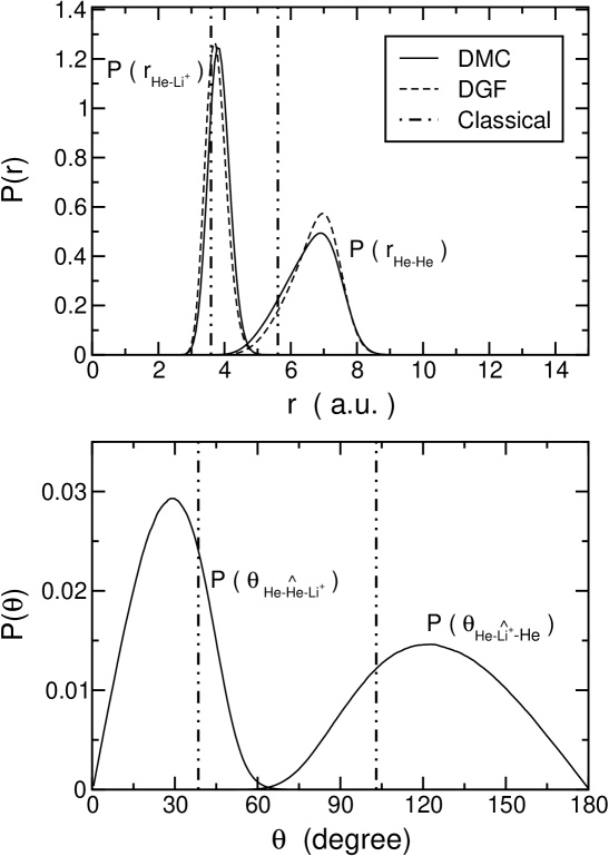
Figure 3: The distribution functions for the Li⁺He₂ calculated via the DMC (solid line) and the DGF (dashed line) methods. In the upper panel we report the pair distribution functions of the relative atom-atom distances while the lower panel shows the distribution functions for the internal angles. The (r,$\theta$) values obtained classically are given as vertical lines in the two panels.

We therefore begin by looking at the average values of the radial distances and angles (see Table II) which, together with the corresponding standard deviations, describe the ground state of the trimer and clearly confirm its having a rather floppy structure: on the other hand, the Li⁺ species still is undoubtedly seen by our calculations to coordinate the two He atoms at a distance determined within 0.3 a₀. Information on the overall geometrical features of the trimer is further gained from the radial and angular distributions shown in Fig. 3, where the values obtained with the classical optimization are also reported as vertical lines. DMC and DGF results are substantially concident and the small differences are mainly due to the bias contained in our DMC distributions. We notice that the floppiness of the system is particularly evident when looking at the distribution function related to the He-He distance, whose standard deviation is more than twice larger than the one for the Li⁺-He bonds. The classical values obtained in the structure optimization are also closer to the quantum average values obtained for the Li⁺-He distances.

In the classical description we do find that the ground state of the trimer is depicted by an isosceles triangle, with the two shorter sides associated to the two Li⁺-He distances and a longer one corresponding to the He-He distance. On the other hand, the real quantum system cannot be described by one single structure only, and its distribution functions correctly show a delocalized triatom with a dominant contribution from the collinear arrangement. The image of a structure with the Li⁺ coordinating the two He atoms at a rather well defined distance (notice the compact distribution function related to Li⁺-He distances) is not completely lost in the quantum description, meaning that the presence of the strong ionic forces from Li⁺ is reducing the degree of delocalization which is always present in the pure He aggregates. This change determines the more rigid structure of the system in the sense that now the He atoms are more strongly coordinated directly to the Li⁺ impurity (see next section on the larger clusters).

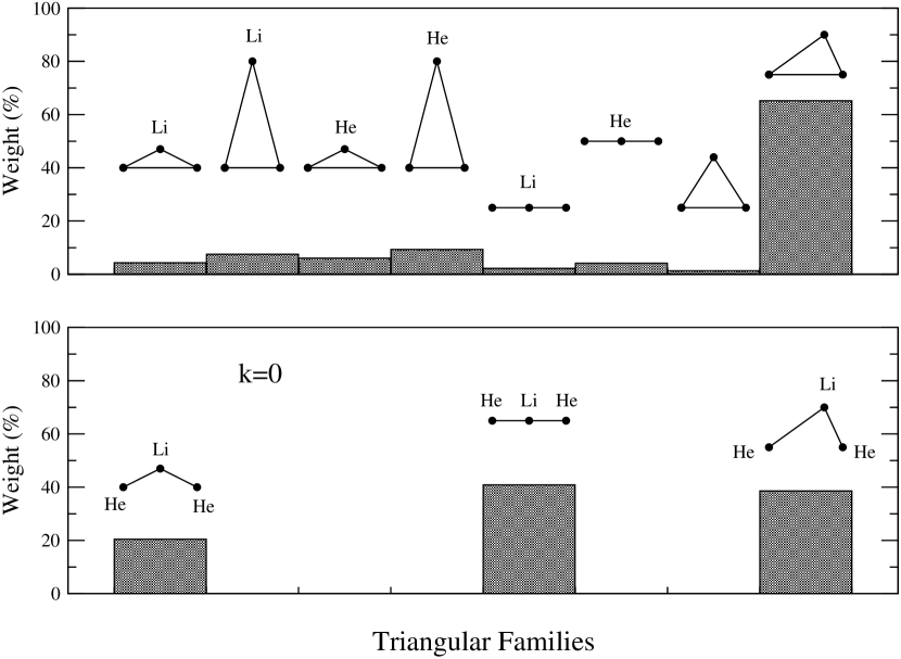
Figure 4: DGF description of the ground state of the Li⁺He₂ in terms of triangular families. In the upper panel we report those basis functions (as percentage with respect to the total number of basis functions) corresponding to the different types of triangular configurations sketched in that panel. In the lower panel we show the three configurations that contribute the most to the ground state of the trimer.

We carried out an additional analysis of the structural features of the trimer by taking advantage of the DGF pseudo-weights 11 , which allow us to pictorially describe the trimer in terms of types of triangular arrangements. In the upper panel of Fig. 4 we thus report all the employed basis set functions, grouped according to the triangular family to which they belong, and in the lower panel of the same figure we report the ‘weight’ of the dominant families when describing the ground state of the trimer. We can thus easily identify the most important arrangement to be given by the ‘flat’ isosceles, the collinear (with the the impurity in the middle) and the scalene triangles, while all other possibilities do not contribute in a significant way. Again, we find that we cannot associate the system to one unique structure. while the marked delocalization features are now mainly related to the He-He binding and less to the Li⁺-He ionic forces; hence we see that a conventional structure with the Li⁺ coordinating the two He atoms can still be qualitatively identified. In the next section we shall further discuss how the situation evolves with the addition of more He atoms and to which extent the classical results can be still seen to qualitatively correspond to the quantum description of their structures surrounding the ionic dopant.

V Energetics and structures of $\rm{\mathbf{Li^{+}-He_{n}}}$ (3 $\rm{\mathbf{\leq n\leq}}$ 30) clusters from quantum and classical calculations

We start now to discuss the energetics and the geometrical features of the larger $\mathrm{Li^{+}He}_{n}$ clusters with $n\geq 3$. Up to $n=10$, infact, it was still possible to also carry out quantum DMC calculations which are not too demanding in terms of CPU-time. Hence, for clusters of such a size we can make a direct comparison between our quantum findings and the classical optimization results we obtained via the combination of the OPTIM procedure walesOPT with a random search for the minimum energy structures (see for details refs. nostroArH ; nostroNeH ). In Table III we report the results for the energetics. The left part of that table shows the minimum potential energies obtained by means of the classical optimizations (column labeled ’classical’) in comparison with the corresponding DMC ground state energies (column labelled ’quantum’). The differences between the two sets of values are due to the ZPE effects of the nuclear motions: in the third column we also display the ZPE value for each cluster as a percentage of the well depth. The amount of the ZPE effects increases as the cluster grows, since the incresing addition of He atoms brings the ZPE percentage from about 20% for $\mathrm{Li^{+}He_{2}}$ to more than 40% for the last cluster studied here with the quantum DMC method ($\mathrm{Li^{+}He_{20}}$). On the right part of Table III we report the total energies relative to the loss of one He atom between the pairs of $\mathrm{Li^{+}He}_{n}$ and $\mathrm{Li^{+}He}_{n-1}$ clusters, calculated both with the classical and quantum methods. We notice that the evaporation energy is drastically reduced when passing from the cluster with n=6 to that with n=7 and correspondingly the ZPE percentage value increases most markedly (more than 3%). We can then surmise that the structure with n=6 is a particularly stable cluster as we shall further discuss below.

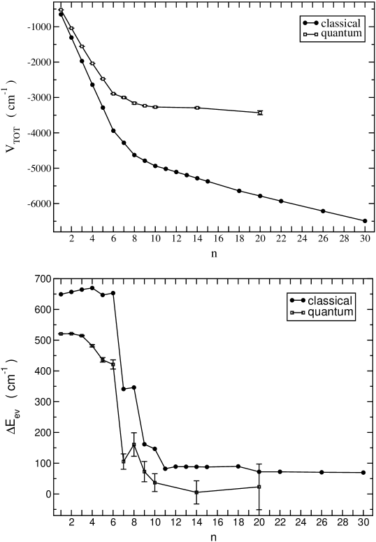
Figure 5: Upper panel: total energies (in cm^-1) as a function of the number n of helium atoms in $\mathrm{Li^{+}H_{n}}$ from classical optimizations (filled-in circles). Lower panel: single helium atom evaporation energies, $\Delta\mathrm{E=-\left[E(Li^{+}He_{n})-E(Li^{+}He_{n-1})\right]}$ in $\mathrm{cm}^{-1}$, as a function of the number n of helium atoms in $\mathrm{Li^{+}He_{n}}$ from the classical optimizations (filled-in circles). The quantum results are given in both panels in open squares showing their corresponding numerical level of confidence.

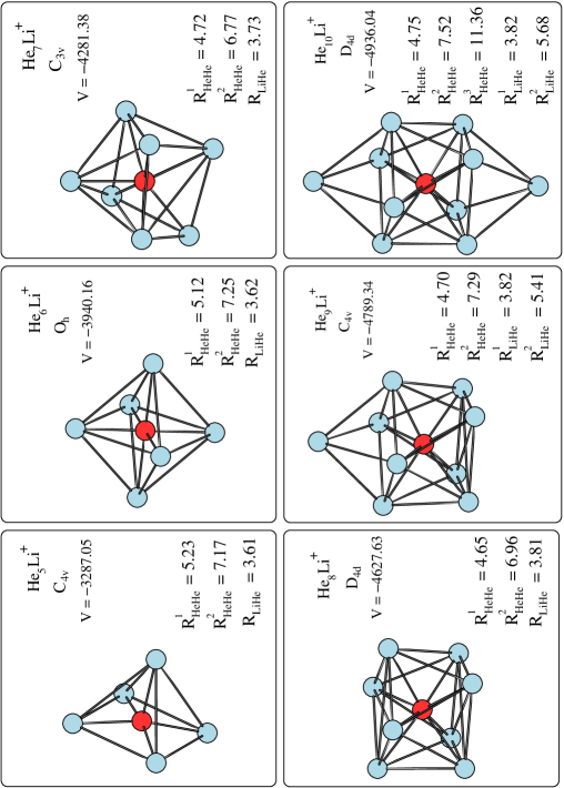
Figure 6: Optimized lowest energy structures obtained with the classical minimizations for $\mathrm{Li^{+}He_{n}}$ with n from 5 to 10.

The data presented in Table III are pictorially reported in the two panels of Fig. 5 where the energies are plotted as functions of the number n of He atoms in each cluster. From the lower panel of Fig. 5 we can see the similar behaviour shown by the $\Delta E_{ev}$ values up to $n=6$ while for $7\leq n\leq 10$ both classical and quantum effects make the two curves show a marked drop in values. The single He atom evaporation energies, $\Delta E_{ev}=-\left[E(\mathrm{Li^{+}He}_{n})-E(\mathrm{Li^{+}He}_{n-1})\right]$, (filled-in circles for the classical calculations and open square for those obtained with the DMC method) are plotted up to $n=30$ (DMC resul ts up to $n=20$): again the two curves show very similar behaviour, both presenting the same abrupt energy drop at $n=7$ and $n=9$. In contrast with what we found in our analysis of H^-He_n clusters nostroHeH , the step-like structure shown by the classical treatment is now also present in the quantum calculations. Given such a correspondence between the classical and quantum description for these smaller clusters it then becomes reasonable to try to explain the sudden energy jumps of Fig. 5 by looking at the lowest energy structures found with the classical minimizations (see Fig. 6). In that figure we also report the corresponding symmetry groups, the total energy (in cm^-1), and the relevant distances between atoms (in a.u.). We therefore see that the $\mathrm{Li^{+}He_{6}}$ has the very symmetrical octahedral geometry (see second panel in the upper part of the figure) where all the He atoms are equivalently coordinated to the central Li⁺ at a distance very close to the $\mathrm{R_{eq}}$ (3.58 a₀) of the $\mathrm{Li^{+}He}$ PEC. On the other hand, when moving to the $\mathrm{Li^{+}He_{7}}$, the repulsive forces acting between the rare gas species do not allow any more for such a symmetrical arrangement around the $\mathrm{Li^{+}}$ ion and the net effect is that of decreasing the energy contributions from the interactions between each He atom and the positive ion, i.e. the $\mathrm{Li^{+}He}$ distance becomes larger, as one can see in Fig. 6 from the reported $\mathrm{R_{LiHe}}$ values. Similar reasoning can be applied to explain the second energy step between $\mathrm{n=8}$ and $\mathrm{n=9}$: the evaporation energy gives the mean value of the energy necessary to remove any of the He atoms and the presence of a non-equivalent rare gas atom in the apical position in $\mathrm{Li^{+}He_{9}}$ (see second panel in the lower part of Fig. 6) causes a significant decrease of the evaporation energy with respect to its value for the $\mathrm{Li^{+}He_{8}}$ cluster. Finally, for $\mathrm{Li^{+}He_{10}}$ the lowest energy structure we obtained with the classical minimization corresponds to the symmetrical bicapped square antiprism geometry. Hence, by using the classical geometries and energy minimization procedures, we found three relatively more stable structures for clusters with $n$=6,8 and 10, in correspondence with symmetrically compact structures. However, we cannot associate the closing of a solvating ‘shell’ to the clusters with $n$=6 and $n$=8 because they do not constitute as yet a possible core around which the larger clusters grow.

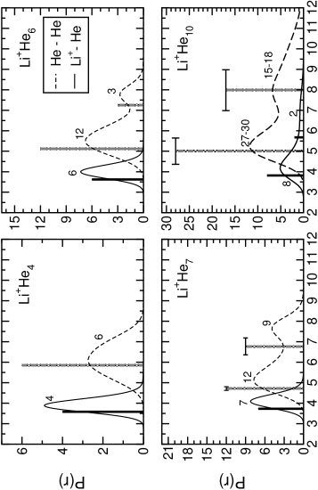
Figure 7: Distribution functions of the atom-atom relative distances P(r), normalized to the number of ’connections’ between the atoms in each cluster, as a function of the distance r (in a.u.). DMC calculations for the $\mathrm{Li^{+}He_{n}}$, $\mathrm{n=4,6,7,10}$. In all panels the solid lines are for the $\mathrm{Li^{+}-He}$ distances while the dashed ones refer to the $\mathrm{He-He}$ distances. The vertical lines indicate the computed mean values of the atom-atom distances (solid lines for $\mathrm{Li^{+}-He}$ and gray lines for $\mathrm{He-He}$) of the optimized structures from the classical calculations, with their height showing the number of bonds associated with that distance (marked also by its spread value on top of each “stick”). The presented numbers in each panel give the corresponding quantum density of bonds within each computed profile.

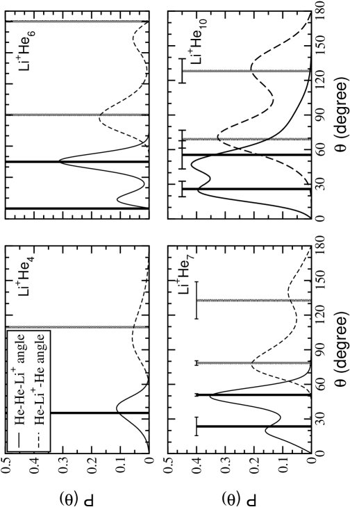
Figure 8: Angular distribution functions $\mathrm{P(\theta)}$, obtained with the DMC calculations for the $\mathrm{Li^{+}He_{n}}$, $\mathrm{n=4,6,7,10}$. In all the panels the solid line is for the $\mathrm{He-He-Li^{+}}$ angles and the dashed line for the $\mathrm{He-Li^{+}-He}$ angles. The vertical lines indicate the various mean values of the angles (solid lines for $\mathrm{He-He-Li^{+}}$ and dashed lines for $\mathrm{He-Li^{+}-He}$) of the optimized structures given by the classical calculations. The notation is the same as in Figure 7

The correspondence between classical and quantum structural pictures is clearly well reproduced if we now compare the quantum distribution functions with the classical results for the relative distances and angles. In Fig. 7 we report the DMC atom-atom distribution functions for the $\mathrm{Li^{+}-He}$ and $\mathrm{He-He}$ distances within each $\mathrm{Li^{+}He}_{n}$ cluster, normalized to the total number n of possible ’connections’ between $\mathrm{Li^{+}}$ and He atoms (solid lines) and to the total number $N=n(n-1)/2$ possible ’connections’ between the n He atoms (dashed lines). In this way we can make a direct comparison between the quantum calculations and the lowest energy geometrical structures obtained with the classical optimizations where the conventional picture of direct bonds existing between localized, point-like, partners can be used. In that figure we also report the classically optimized distances: we have grouped together sets of close values and have given as horizontal bars their statistical standard deviations: each set has a height proportional to the number of distances which have the same value. Finally, the displayed numbers are the values of the integration along r for each broad peak in the quantum distribution functions and represent the number of bonds within atoms which are in the given distance range under each integration. In Fig. 7 we report the results for four selected clusters ($\mathrm{n=4,6,7,10}$) which we shall use in our discussion: we also obtained similar results for all the other clusters. When we look at the panel showing the $\mathrm{Li^{+}He_{4}}$ clusters in the upper left of Figure 7, we see that the DMC distribution function for the $\mathrm{Li^{+}-He}$ distance peaks at 3.88 a.u. while the classical distances are represented by one ’stick’ at 3.59 a.u. whose height is 4, equal to the value of the area under the quantum distribution (solid line); we see also that the DMC distribution function for the $\mathrm{He-He}$ distance peaks at 6.13 a.u. while the classical distances are represented by one ’stick’ at 5.85 a.u. whose height is 6 (which is the value of $N=n(n-1)/2$, with $n=4$) a number which is indeed equal to the value of the area under the quantum distribution (dashed line). For the larger clusters (see the other panels of the same figure) the number of distinct sets of distances increases, but still the agreement between classical and quantum findings concerning the number of corresponding distances remains very good. Although the mean values are different as a consequence of the very diffuse behaviour of the wavefunctions in such weak interatomic potentials, we can clearly see that the classical results essentially provide the same qualitative structural picture. In order to compare even more in detail the classical and quantum results, we report in Fig 8 the DMC angular distribution functions P($\theta$) for the angles centered at the Li⁺ ion and at any of the He atoms together with the results from classical optimization: we see again that the agreement between quantum and classical values (vertical lines) indeed remains very close, at least at the qualitative level.

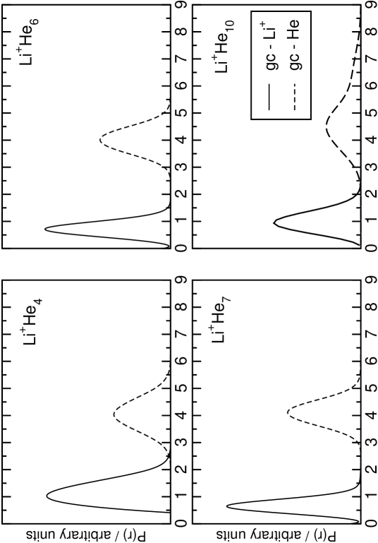
Figure 9: DMC distribution functions of the distances of the He atoms (dashed lines) and of the Li⁺ (solid lines) from the geometrical center (gc) for selected clusters as functions of the distance r (in a.u.). The density distributions are normalized so that the area under them is unitary

These findings allow us to make further comments on the microsolvation process that occurs when the Li⁺ is inserted in a small He cluster. Both the classical and the quantum treatments concur in locating the Li⁺ impurity inside the He_n moiety as one can clearly see from Figure 9 where we report the DMC distribution functions P(r) of the Li⁺ (solid lines) and of the He atoms (dashed lines) from the geometrical center of each $\mathrm{Li^{+}He}_{n}$ cluster. This quantity is defined as:

$$\mathbf{r}_{gc}=\frac{1}{N}\sum_{i=1}^{N}\mathbf{r}_{i},$$ (7)

where N runs over the total number of atoms in the cluster. The Li⁺ is always closer to the geometrical center with respect to the He atoms, and when the cluster size increases the corresponding distribution functions have reduced overlap, thereby showing that the cluster growth is accompanied by the slow “dropping” of the Li⁺ towards the geometrical center of the latter

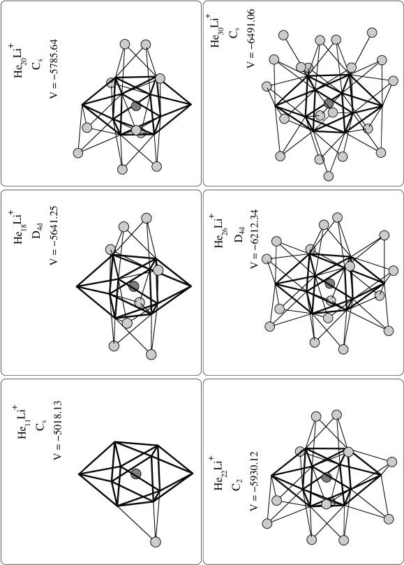
Figure 10: Optimized lowest energy structures obtained with the classical minimizations for $\mathrm{Li^{+}He_{n}}$ with $\mathrm{n=11,18,22,26,30}$. The central polyhedron including the Li⁺ ion represents the $\mathrm{Li^{+}He_{10}}$ core.

Finally, we carried out classical optimizations for larger clusters $\mathrm{Li^{+}He_{n}}$ (n=11-15, 18,20,22,26,30) in order to better confirm what we have observed in the smaller ones; the lowest energy geometries for a selection of them are reported in Fig. 10. For all the clusters under inspection, the growth occurs around the highly symmetric $\mathrm{Li^{+}He_{10}}$ core represented by the bicapped square antiprism polyhedron enclosing the Li⁺ impurity and drawn with thicker lines in the figure. The additional He atoms are now being placed further away from the impurity without perturbing the structure of the $\mathrm{Li^{+}He_{10}}$ moiety which therefore seems to constitute the first solvation shell of the atomic ion. We expect that the He atoms outside the shell will be characterized by a greater delocalization and weaker interactions with the central Li⁺ that the less shielded inner core of ten atoms. From now on we expect, therefore, that the cluster will grow by adding more solvent atoms in a nearly isotropic fashion driven mainly by He-He interaction and we surmise that the binding energies of each atom will become increasingly similar to those of a pure He cluster. Correspondingly, the evaporation energy (see Fig. 6) now shows a markedly different behaviour with respect to what happens in the smaller clusters with n $\leq$ 10: the step-like feature disappears, to be substituted by a plateau giving us the average energy needed to remove one of the nearly equivalent external He atoms.

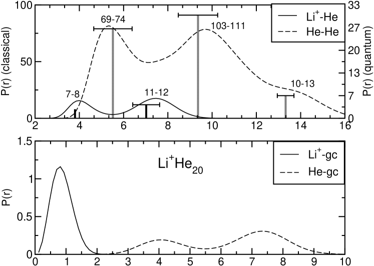
Figure 11: Quantum DMC distributions for the Li⁺He₂₀ moiety. Upper panel: atom-atom distance distributions compared with classical distance values as in Figure 8. Lower panel: distance distributions with respect to the geometric center of the cluster as in Figure 9.

This expected result is also shown by the quantum calculations (see Figure 5, lower panel) and is also borne out by the corresponding quantum distributions of the helium adatoms given by the data of Figure 11, where our DMC calculations for the $\mathrm{Li}^{+}(\mathrm{He})_{20}$ clusters are reported: one clearly see there that the radial distributions associated with the He distances from the Li⁺ moiety show a set of more compact values related to the first shell of about 10 adatoms and a further distribution at larger distances (and broader than the first one) associated with the outer atoms that are chiefly bound by dispersion and by strongly screened induction interactions.

VI Conclusions

In the present work we have analized the solvation process of a Li⁺ ion in pure bosonic Helium clusters in order to extend to a larger number of atoms the studies we had already carried out in previous work on the smaller aggregates 8 . Here a combination of classical energy minimization techniques and of “exact” quantum Monte Carlo methods have been employed in order to describe the structure and the energetics of the Li⁺(He)_n clusters with $n$ up to 30 (20 for DMC calculations), employing always a description based on the sum-of-potential approximation.

The basic approximation which this study relies on is that of calculating the full cluster interaction as a sum of pairwise potentials. Although the error introduced by this assumption is in general found to be (in absolute terms) larger in ionic systems than in neutral ones, its relative weight remains rather small 8 . Thus, we believe that the resulting stuctures and energies would not be substantially altered by the correct use of a full Many-Body potential (see for example, the discussion in Ref. 29 for the similar situations of H^- and Cl^- in Rg clusters and our calculations in Ref. 8 ).

We have therefore shown that:

1. the Li⁺ is fully solvated inside larger ⁴He clusters as already indicated by our earlier work on very small aggregates 8 ;

2. the ionic Li⁺ core does not form preferential “molecular cores” with surrounding He atoms but rather that the helium adatoms remain equivalently bound within each solvation shell to the central, solvated lithium ion that persists in carrying the positive charge for more than 98% 8 .

3. the ZPE corrections play a role in such systems, albeit strongly reduced with respect to the one found in neutral aggregates: this means that, at least in the initial solvation shell, the quantum adatoms are less delocalized and that the lithium-helium direct “bonds” are nearly rigid, classical structures;

4. the classical optimization procedures can provide structural details which are reasonably close to those given by the quantum DMC calculations and can yield for ionic moieties the same structural picture as that given by the quantum treatment.

Furthermore, our comparison of single particle evaporation energies given by classical and quantum results suggests in both cases the formation of an initial shell of about ten He atoms which are more strongly bound to the central ion. On the other hand, beyond that initial shell the cluster growth appears to be chiefly driven by He-He interactions, albeit at energies which are initially still kept larger than those of the neutral systems by the additional presence of the induction field due to the central ionic core. This bahevior may be compared to that of Na⁺ and K⁺ doped Helium clusters 5a where the first solvation shells were found to be of 9 and 12 atoms respectively.

Table 1: Bound states supported by the three pair potentials for Li⁺-He. Values in the first column are taken from Ref. 19 . The values in the second and third column have been calculated by us. All quantities are in units of cm^-1

$\nu$	CCSD(T) (aug-cc-pV5Z)	MP4 (cc-pV5Z)	ATT
0	-519.975	-515.225	-496.319
1	-311.396	-307.280	-289.972
2	-165.739	-161.536	-150.728
3	-75.323	-70.519	-67.050
4	-27.55	-23.130	-23.902
5	-7.191	-4.642	-5.905
6	-0.925	-0.356	-0.669
7	-0.007	-	-0.002
$D_{e}$	649.155	643.980	627.408
ZPE	129.180 (19.90 %)	128.755 (19.99 %)	131.090 (20.89 %)

Table 2: Comparison of the results for the ground state of (LiHe₂)⁺ obtained with both DMC and DGF methods. The energies are in cm^-1, the distances in a.u., the angles in degrees and the areas S in a.u.². The ZPE is expressed as percentage of the the total well depth for the trimer D_e = 1306.02 cm^-1 (from classical optimization).

	Ev=0	ZPE	rHe-He	r${}_{He-Li^{+}}$	$\theta_{\widehat{He}}$	$\theta_{\widehat{Li^{+}}}$	$\sqrt{<S^{2}>}$
DMC	-1041.7 $\pm$ 0.68	20.24 %	6.59 $\pm$ 0.81	3.83 $\pm$ 0.32	28.43 $\pm$ 12.20	123.88 $\pm$ 24.01	5.54 $\pm$ 1.84
DGF	-1042.45	20.18 %	6.69 $\pm$ 0.73	3.75 $\pm$ 0.32	26.94 $\pm$ 17.69	127.36 $\pm$ 27.99	5.24

Table 3: Minimum total energies and single-particle evaporation energies using classical and quantum treatments for the nuclear motion. ZPE (%) means: $\mathrm{\left[\left(V^{TOT}_{classical}-V^{TOT}_{quantum}\right)/V^{TOT}_{classical}\right]\cdot 100}$. $\mathrm{\Delta E_{evap}}$ means: $\mathrm{-\left[V^{TOT}\left(Li^{+}(He)_{n}\right)-V^{TOT}\left(Li^{+}(He)_{n-1}\right)\right]}$ The quantum evaporation energy for $n$=14 has been calculated using the formula $E_{evap}(14)=(E(10)-E(14))/4$ and for $n$=20 $E_{evap}(20)=(E(14)-E(20))/6$

. n $\mathrm{V^{TOT}}$ $\mathrm{\Delta E_{evap}}$ classical quantum ZPE (%) classical quantum 2 -1306.0 -1041.7 $\pm$ 0.7 20.2 656.8 521.1 $\pm$ 0.7 3 -1970.5 -1556.3 $\pm$ 0.8 21.0 664.4 514.6 $\pm$ 1.5 4 -2640.1 -2038.1 $\pm$ 2.9 22.8 669.6 481.7 $\pm$ 3.7 5 -3287.0 -2474.1 $\pm$ 4.6 24.7 646.9 436.1 $\pm$ 7.5 6 -3940.2 -2895.3 $\pm$ 10.3 26.5 653.1 421.1 $\pm$ 14.9 7 -4281.4 -3000.7 $\pm$ 14.7 29.9 341.2 105.4 $\pm$ 25.0 8 -4627.6 -3161.5 $\pm$ 23.5 31.7 346.2 160.8 $\pm$ 38.2 9 -4789.3 -3234.3 $\pm$ 9.5 32.5 161.7 72.8 $\pm$ 33.0 10 -4936.0 -3271.2 $\pm$ 19.5 33.7 146.7 36.9 $\pm$ 29.0 14 -5284.2 -3292.4 $\pm$ 18.1 37.7 88.4 5.3 $\pm$ 37.6 20 -5785.6 -3432.5 $\pm$ 56.1 40.7 72.2 23.3 $\pm$ 74.2