Core-periphery organization of complex networks

Abstract

Networks may, or may not, be wired to have a core that is both itself densely connected and central in terms of graph distance. In this study we propose a coefficient to measure if the network has such a clear-cut core-periphery dichotomy. We measure this coefficient for a number of real-world and model networks and find that different classes of networks have their characteristic values. For example do geographical networks have a strong core-periphery structure, while the core-periphery structure of social networks (despite their positive degree-degree correlations) is rather weak. We proceed to study radial statistics of the core, i.e. properties of the $n$-neighborhoods of the core vertices for increasing $n$. We find that almost all networks have unexpectedly many edges within $n$-neighborhoods at a certain distance from the core suggesting an effective radius for non-trivial network processes.

I Introduction

All systems consisting of pairwise-interacting entities can be modeled as networks. This makes the study of complex networks one of the most general and interdisciplinary areas of statistical physics mejn:rev ; ba:rev ; doromen:book . One of the most important gains of the recent wave of statistical network studies is the quantification of large-scale network topology luc:rev ; mejn:rev . Now, with the use one just a few words and numbers, one can state the essential characteristics of a huge network—characteristics that also say something about how dynamical systems confined to the network will behave. A possible large-scale design principle is that one part of the network constitutes a densely connected core that also is central in terms of network distance, and the rest of the network forms a periphery. In, for example, a network of airline connections you would most certainly pass such a core-airport on any many-flight itinerary. It is known that a broad degree distribution can create a core having these properties chung_lu:pnas . In this paper we address the question if there is a tendency for such a structure in the actual wiring of the network. I.e., if one assumes degree to be, to a large extent, an intrinsic property of the vertices, then is the network organized with a distinct core-periphery structure or not? To give a quantitative answer to this question our first step is to find a core with the above mentioned properties—being highly-interconnected and having a high closeness centrality sab:clo (the inverse average distance between a vertex in the core and an arbitrary vertex). Once such a subgraph is identified we calculate its closeness centrality relative to the graph as a whole, and subtract the corresponding quantity for the ensemble of random graphs with the same set of degrees as the original network (cf. Ref. maslov:pro ). If the resulting coefficient is positive the network shows a pronounced core-periphery structure. Once the core and periphery are distinguished one may proceed to investigate their structure. We look at the statistical properties of the $n$-neighborhoods (the set of vertices on distance $n$) of the core vertices. By such radial statistics we can draw conclusions for the respective function of the core and periphery. This paper starts by defining the core-periphery coefficient and measure it for real-world networks of numerous types, then proceeds by discussing and measuring radial statistics.

Table 1: The network sizes $N$ and $M$, the core-periphery coefficient $c_{\mathrm{cp}}$ and the relative assortative mixing coefficient $\Delta r$ for a number of networks. In the interstate network the vertices are American interstate highway junctions and two junctions are connected if there is a road with no junction in between. The pipeline network is a similar network of junctions and gas pipes. In the street networks the vertices are Swedish city street segments connected if they share a junction. In the airport data (obtained from IATA www.iata.org) the vertices are airports and the edges represent airport pairs with a non-stop flight connection. The Internet figures are averages of 15 AS-level graphs constructed from traceroute searches. The arXiv, board of directors and Ajou students are constructed one-mode projections from affiliation networks (where links goes from persons to e-prints, corporate boards and university classes respectively). The student network is averaged over graphs for 16 semesters. One edge represent two students taking at least three classes together that semester. The high school, prisoner and social scientist networks are gathered from questionnaires—an edge means that two persons have listed each other as acquaintances. The high school data are averaged over 84 individual schools. In the electronic communication networks one edge represent that at least one of the vertices has contacted the other over some electronic medium. In the nd.edu data the vertices are HTML documents and the edges are hyperlink. The citation graph is constructed from preprints in the field of high-energy physics kdd:hep (see: http://www.cs.cornell.edu/projects/kddcup/datasets.html). In the software dependency graph the vertices are software packages and an edge means that one package needs the other for its proper function. The food webs are networks of water-living species and an edge means that one species prey on the other. For the protein networks an edge means that two proteins bind to each other physically. The metabolic and “whole cellular” networks consist of chemical substances and edges indicating that one molecule occur in the same reaction as the other (the values for these networks are averages over 43 organisms from different domains of life).

Network		Ref.	$N$	$M$	$c_{\mathrm{cp}}$	$\Delta r$
Geographical networks	Interstate highways		935	1315	0.231(1)	0.0851(5)
	Pipelines	gast:effi	2999	3079	0.180(2)	0.073(2)
	Streets, Stockholm	rosv:city	3325	5100	0.255(1)	0.080(1)
	Streets, Göteborg	rosv:city	1258	1516	0.040(3)	0.019(3)
	Airport		449	2795	0.0523(3)	0.0910(3)
	Internet	vesp:inet	1968(66)	4051(121)	0.045(2)	0.009(3)
One-mode projections of	arXiv	mejn:scicolpre1	48561	287570	–0.08(3)	0.361(3)
affiliation networks	Board of directors	davis	6193	43074	–0.037(2)	0.280(2)
	Ajou University students	our:ajou1 ; our:ajou2	7285(128)	75898(6566)	–0.08(1)	0.66(4)
Acquaintance networks	High School friendship	addh	571(43)	1078(85)	0.006(7)	0.19(1)
	Prisoners	mcrae:prison	58	83	–0.043(2)	0.264(2)
	Social scientists	freeman:eiec	34	265(35)	-0.002(4)	0.10(1)
Electronic communication	e-mail, Ebel et al.	bornholdt:email	39592	57703	–0.229(4)	–0.001(4)
	e-mail, Eckmann et al.	eckmann:dialog	3186	31856	–0.091(2)	–0.034(2)
	Internet community, nioki.com	nioki	49801	239265	–0.014(2)	0.007(2)
	Internet community, pussokram.com	pok	28295	115335	–0.183(5)	–0.005(5)
Reference networks	WWW, nd.edu	ba:dia	325729	1090108	–0.027(3)	–0.003(3)
	HEP citations		27400	352021	–0.10(1)	0.03(1)
Software dependencies	GNU / Linux	mejn:mix	504	793	–0.155(1)	–0.087(1)
Food webs	Little Rock Lake	martinez:rock	92	960	0.005(6)	–0.0141(6)
	Ythan Estuary	ythan1	134	593	–0.020(1)	–0.0153(9)
Neural network	C. elegans	cenn:brenner	280	1973	0.040(6)	0.0222(7)
Biochemical networks	Drosophila protein	droso:pin	2915	4121	–0.035(2)	0.003(1)
	S. cervisiae protein	pagel:mips	3898	7283	–0.249(1)	–0.069(1)
	S. cervisiae genetic	pagel:mips	1503	5043	–0.0646(7)	–0.101(1)
	Metabolic networks	jeong:meta	427(27)	1257(88)	–0.002(6)	0.006(1)
	Whole cellular networks	jeong:meta	623(32)	1752(103)	–0.004(6)	–0.001(2)

II Measuring the core-periphery structure

In this paper we assume the network to be represented as a graph $G=(V,E)$ with a set $V$ of $N$ vertices and a set $E$ of $M$ undirected and unweighted edges. (It is straightforward to generalize our analysis to weighted networks.) Since our analysis requires the network to be connected we will henceforth identify $G$ with the largest connected component of the network (in all mentioned cases this component will constitute almost the entire network). We also remove self-edges and multiple edges.

II.1 Rationale and definition of the core-periphery coefficient

The notion of network centrality is a very broad and many measures have been proposed to capture different aspects of the concept harary . One of the simplest quantities is the closeness centrality sab:clo

$$C_{C}(i)=\left(\langle d(i,j)\rangle_{j\in V\setminus\{i\}}\right)^{-1}$$ (1)

of a vertex $i$, where $d(i,j)$ is the distance between $i$ and $j$ (the smallest number of edges on a path from $i$ to $j$). The closeness of a vertex is thus the reciprocal average shortest distance to the other vertices of $V$. This definition is straightforwardly extended to a subset $U$ of vertices

$$C_{C}(U)=\left(\left\langle\langle d(i,j)\rangle_{j\in V\setminus\{i\}}\right\rangle_{i\in U}\right)^{-1}.$$ (2)

So we require a core to be a subgraph $U$ with high $C_{C}(U)$, but also to be a well-defined cluster—i.e. to have comparatively many edges within. Now, if there are many facets of the centrality concept, there are even more algorithms to identify graph clusters, each being a de facto cluster-definition mejn:rev . For simplicity we choose the most rudimentary cluster-definition—the set of $k$-cores. A $k$-core is a maximal subgraph with the minimum degree $k$ (maximal in the sense that if one adds any vertex to a $k$-core it will no longer have a minimal degree $k$). To calculate a sequence of $k$-cores is computationally cheaper (linear in $M$ rama:core ) than more elaborate clustering algorithms. So we let our core $V_{\mathrm{core}}(G)$ be the $k$-core with maximal closeness and define the core-periphery coefficient $c_{\mathrm{cp}}$ as

$$c_{\mathrm{cp}}(G)=\frac{C_{C}[V_{\mathrm{core}}(G)]}{C_{C}[V(G)]}-\left\langle\frac{C_{C}[V_{\mathrm{core}}(G^{\prime})]}{C_{C}[V(G^{\prime})]}\right\rangle_{G^{\prime}\in\mathcal{G}(G)},$$ (3)

where $\mathcal{G}(G)$ is the ensemble of graphs with the same set of degrees as $G$. The sequence of $k$-cores is not necessarily unique. We maximize $C_{C}(U)$ over $m_{\mathrm{seq}}$ different sequences. In practice different runs almost always yield the same core, and the value of $m_{\mathrm{seq}}$ seems to matter little. The $m_{\mathrm{null}}$ elements of $\mathcal{G}(G)$ can be obtained by randomization of $G$ in time and space of the order of $M$ roberts:mcmc . In this paper we use $m_{\mathrm{null}}=1000$ and $m_{\mathrm{seq}}=10$ for networks with $N<5000$, and $m_{\mathrm{null}}=50$ and $m_{\mathrm{seq}}=3$ for $N\geq 5000$.

The correlation of degrees at either side of an edge is an informative structure to study maslov:pro ; mejn:assmix ; pas:inet . To some extent one can see degree-degree correlations as a local version of the core-periphery structure—when there are positive degree-degree correlations, at least some subgraphs of the network will have a well-defined core and periphery. Such clusters need not be centrally positioned in the graph as a whole, so while the degree-degree correlations says something about if the graph can be separated into densely and sparsely connected regions, the core-periphery structure gives information of the relative position of such regions. A common way to quantify the average degree-degree correlations is to measure the assortative mixing coefficient mejn:assmix

$$r=\frac{4\langle k_{1}\,k_{2}\rangle-\langle k_{1}+k_{2}\rangle^{2}}{2\langle k_{1}^{2}+k_{2}^{2}\rangle-\langle k_{1}+k_{2}\rangle^{2}},$$ (4)

where $k_{i}$ is the degree of the $i$’th argument of a edge as it appear in a list of $E$. Now, our null-model is a random graph conditioned to have the same degree sequence as the original graph. In other words, just as for the core-periphery structure, we consider the deviation from our null model and measure the relative assortative mixing coefficient

$$\Delta r(G)=r(G)-\left\langle r(G^{\prime})\right\rangle_{G^{\prime}\in\mathcal{G}(G)}.$$ (5)

II.2 Numerical results for real-world networks

In Table 1 $c_{\mathrm{cp}}$ and $\Delta r$ are displayed for a number of real-world networks. We find that the core-periphery structure and relative degree-degree correlations follow the different classes of networks rather closely. Furthermore the core-periphery structure and degree-degree correlations seem to be quite independent network structures in practice. For example, geographically embedded networks have a clear core-periphery structure and weakly positive degree-degree correlations; social networks derived from affiliations have slightly negative $c_{\mathrm{cp}}$-values but very high $\Delta r$-values; networks of online communication have markedly negative $c_{\mathrm{cp}}$ and rather neutral degree-degree correlations. Most geographically embedded networks have the function of transporting, or transmitting, something between the vertices. Networks with a well-defined core (which most paths pass through) and a periphery (covering most of the area) are known to have good performance with respect to communication times gast:effi . Also networks of airline traffic gui:air and the hardwired Internet zhou:rich ; vesp:inet are known to have well-defined cores due to traffic-flow optimization. The class of one-mode projection networks (social networks constructed by linking people that participate in something—movies, scientific research, etc.—together) show slightly negative $c_{\mathrm{cp}}$-values. This can, at least for the data sets of scientific coauthors mejn:scicolpre1 and fellow students of a Korean university our:ajou1 ; our:ajou2 , be explained by that there is a grouping of the people on the basis of specialization (and, in student networks, also in grade) and thus no well-defined core. We note that this group of networks have very high $\Delta r$ values. The interview based acquaintance networks show rather neutral $c_{\mathrm{cp}}$-values and positive $\Delta r$ suggesting that there is a degree of independence between. This is quite similar to the one-mode projections, which probably is not a coincidence—there is a strong correlation between acquaintance ties and the organizations people are affiliated with. The vertices in electronic communication networks are also people but the network structures of these are quite different; the degree-degree correlation is typically slightly negative, as is the core-periphery coefficient. Information networks where the edges refer to supporting information sources (our examples are a subgraph of the WWW and a graph of citations between papers in high-energy physics) can be expected to be grouped into topics, thus the negative $c_{\mathrm{cp}}$. The same explanation applies to the negative $c_{\mathrm{cp}}$ of the software dependency graph. Food webs are other stratified networks where a lack of a well-defined core seems natural. The core of the neural network of C. elegans is a clique (fully connected subgraph) of eight neurons, which accounts for positive $c_{\mathrm{cp}}$ and $\Delta r$ values. The biochemical networks all show negative $c_{\mathrm{cp}}$ values and negative, or neutral, relative assortative mixing coefficients.

II.3 Numerical results for network models

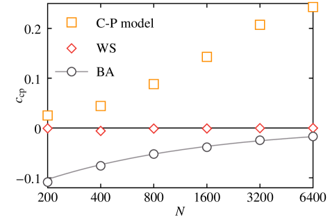
Figure 1: Core-periphery structure of model networks. The Barabási-Albert and Watts-Strogatz networks have $M=2N$. The core-periphery model has the parameter $f_{\mathrm{core}}=0.96$ (i.e. the intended core consists of 4% of the vertices) and $\gamma=3$. All values are averaged over $10^{4}$-$10^{5}$ network realizations. The BA-model line is a fit to an power-law form $\alpha_{0}+\alpha_{1}N^{-\alpha_{2}}$ (this fit gives $c_{\mathrm{cp}}(\infty)=\alpha_{0}=0.004(9)$).

In addition to the real-world networks of Table 1 we also measure the core-periphery coefficient for a few network models. For simple random graphs er:on where $N$ vertices are randomly connected by $M$ edges, defining an ensemble $\mathbb{G}(N,M)$ of graphs, $\mathcal{G}(G)$ is precisely the elements of $\mathbb{G}(N,M)$ with the same degree sequence as $G$. This means that, on average, $c_{\mathrm{cp}}$ will be zero for random graphs. A popular network model is the Barabási-Albert (BA) model ba:model where the graphs are grown by iteratively adding new vertices with edges to old vertices with a probability proportional to the degree of the old vertices. In Fig. 1 we see that $c_{\mathrm{cp}}$ tends to zero (or a value very close to zero) for BA model networks. The BA model has an assortative mixing coefficient $r$ that tends to zero as $N$ grows mejn:assmix . From this one sees that the high-degree vertices are not more interconnected than can be expected from their degrees, and thus that there is no preference in the actual wiring of the network for a well-defined core in the sense of the $c_{\mathrm{cp}}$-coefficient. We also investigate the Watts-Strogatz’ small-world network model wattsstrogatz were one end of the edges of a circulant harary is rewired with a certain probability ($0.01$ in our case). Just as for the BA model $c_{\mathrm{cp}}$ converges to zero (see Fig. 1). This is not so surprising, in the WS model’s starting point, the circulant, every vertex is in the same position. The rewiring procedure does not aggregate vertices to a well-defined core either. Finally we construct a network model with a positive core-periphery coefficient. We start by drawing $N$ power-law distributed random integers in the interval $[2,\infty)$, i.e. the probability for a number $m$ to be drawn is proportional to $m^{-\gamma}$, and sort these numbers in increasing order: $m_{1},\cdots,m_{N}$. These numbers are the desired degrees of the vertices and can be thought of as stubs, or half-edges, that need to be connected. Now we will attempt to make a well-defined core of the vertices $i_{1}^{\mathrm{core}},\cdots,N$, where $i_{1}^{\mathrm{core}}$ is the integer closest to $Nf_{\mathrm{core}}$ (so $f_{\mathrm{core}}$ is a parameter setting the relative size of the core). Then we go through the vertices $i_{1}^{\mathrm{core}},\cdots,N$ in increasing order and for each vertex $i$ try to attach the stubs the vertices $j=i+1,\cdots,N$ (once again in increasing order) as long as the degree of $j$ is less than $m_{j}$. The remaining stubs are paired together randomly and made into edges if they do not form loops or multiple edges. The superfluous stubs are then deleted. For this model $c_{\mathrm{cp}}$ indeed shows positive and growing values, see Fig. 1.

III Radial organization of networks

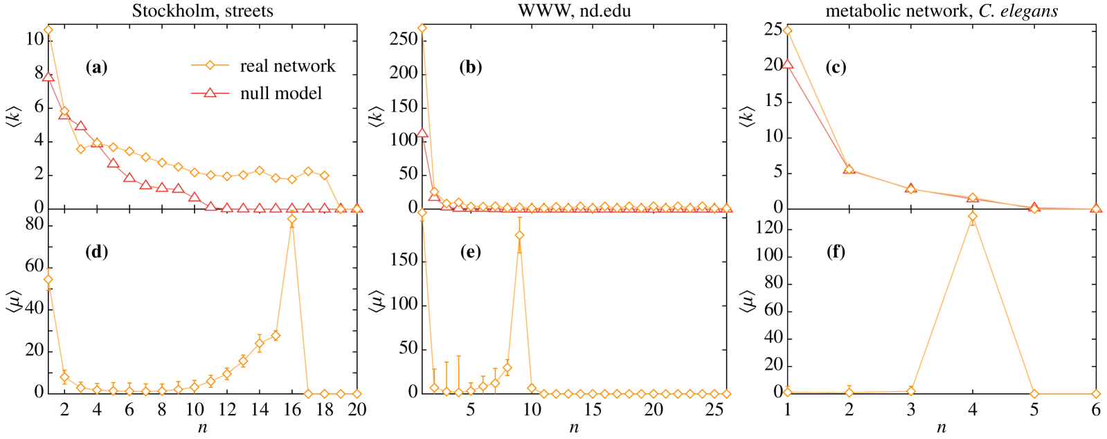
Figure 2: Radial statistics for three real-world networks. (a)-(c) show the average degree $\langle k\rangle$ of the $n$-neighborhoods of the core vertices as a function of $n$ for three real world networks: a network of streets in Stockholm, Sweden rosv:city , a network of hyperlinked web-pages ba:dia and the metabolic network of C. elegans jeong:meta . Curves for our null-model—random networks with the same degree sequence as the original network—are included. In (a)-(c) we plot the number of edges with in the $n$-neighborhood relative to the expected number of edges given the degree sequence of the $n$-neighborhood and the graph as a whole. Lines are guides for the eyes.

A well-defined core is a useful starting point for a radial examination of the network. By plotting quantities averaged over the $n$-neighborhoods (the set of vertices at a distance $n$ of a vertex) of the core vertices as functions of $n$ one can get an idea of the respective purposes of the core and periphery. This kind of statistics is naturally more sensible the stronger the core-periphery structure is. The $c_{\mathrm{cp}}$ construction identifies the most central well-connected core but it does not say whether or not the core make sense—even for slightly negative $c_{\mathrm{cp}}$-values this type of radial statistics may be informative. While authors have focused on the size of the $n$-neighborhoods of random vertices radek ; cohen:tomo —a useful approach to monitor finite-size effects that affects spreading processes such as disease epidemics—we will focus on quantities that we find more informative regarding the relative functions of the core and periphery.

To get a rough view of the radial network organization we plot the average degree of the vertices in the $n$-neighborhood of core-vertices as a function of $n$ in Fig. 2. We include the corresponding results for our null model (random networks constrained to the same degree sequence as the original). The core vertices themselves almost always get higher average degree for the null-model than the real-world networks ($5$-$10\%$ higher for the networks of Fig. 2). For the first neighborhood the situation is reversed—the real-world networks have higher $\langle k\rangle$ than the null-model. Then the degrees are decreasing monotonically; typically faster for the null-model networks. For the street network in Fig. 2(a) $\langle k\rangle$ decreases rather slowly for intermediate $n$; the periphery is thus rather homogeneous. The short average distances of the core, consisting of the streets of the city center, can be attributed to its central geographic position.

One can imagine different functions of the peripheral vertices—either they are just conveying information, traffic, etc. to and from the core; or they are, just as the core-vertices, involved in the general network processes, only less intensely. To understand this we measure the average value of the quantity

$$\mu(i,n)=M(K_{n}(i))/\mathbb{E}M(K_{n}(i))$$ (6)

over the core vertices; $M(K_{n}(i))$ is the number of edges within $i$’s $n$-neighborhood $K_{n}(i)$ and $\mathbb{E}M(K_{n}(i))$ is the expected number of edges in a set of vertices of the same degrees as $K_{n}(i)$ in a random graph of the same degree sequence as the original graph $G$. Calculating of $\mathbb{E}M$ is known to be a hard counting problem BC78 , so we have to rely on the same random sampling as for the $c_{\mathrm{cp}}$-calculation. To save time one can calculate $\mathbb{E}M(K)$ as the average number of edges within the original subgraph $K$ at the same time as the $\mathcal{G}(G)$-sampling of the $c_{\mathrm{cp}}$ calculation. In Fig. 2(d)-(f) we diagram $\langle\mu\rangle(n)$ for our three example networks. Since the core is constructed to be highly inter-connected it is no surprise that $\langle\mu\rangle$ has a peak for small $n$. For the metabolic network of Fig. 2(f) this peak is small. This is due to the exceptionally high degrees $\sim 55$ of the core vertices (including substrates such as H₂O, ATP and ADP)—even in the null-model networks this set of vertices will, for combinatorial reasons, be highly interconnected. For intermediate $n$ the $\langle\mu\rangle$-values are of the order of unity, i.e. there is no overrepresentation of edges between vertices at this distance from the core. But as $n$ increases, $\langle\mu\rangle$ grows to a sharp peak before it eventually drops to zero. This seems like a rather ubiquitous feature (at least it is present in almost all networks of Table 1). We interpret this as that the periphery has both the two functions listed above: To a certain distance from the core (defined by the peak) vertices have similar function and are for this reason connected (and since such small set of, probably, low-degree vertices is unlikely to have many interior edges $\mu$ becomes high); beyond this distance the network consists only of cycle-free branches. This dichotomy—the network in- and outside of the peak radius—is yet more distinct than the core vs. periphery as defined above. On the other hand the outside is functionally rather trivial and (in all cases we study) smaller than the inside (we believe the term “core” is more apt for smaller subgraphs). We note that this peak is not trivially related to the peak in the size of the $n$-neighborhood which is much broader and occurs for smaller $n$.

IV Summary and Discussion

In many networks the properties of vertices are heterogeneously distributed, similarly one can find subgraphs with very different characteristics and function. Perhaps the simplest division of a network is that into a core and a periphery. The core concept has been used in various senses in the past; typically it is defined as a subgraph which is most tightly connected be:cp ; eb:peri or a most central chung_lu:pnas . In this paper we use the rather strong precepts that a core should be both highly interconnected and central. To quantify this idea, we define the core as the $k$-core of highest closeness centrality. Then, to measure the strength of the tendency to have a central and highly connected core, we define a core-periphery coefficient as the normalized closeness centrality of the core minus the same corresponding average value for our null-model (random networks of the same degree sequence as the original network). Different types of networks have their characteristic $c_{\mathrm{cp}}$-values: Geographically embedded networks typically have a positive core-periphery coefficient. We explain this as an effect of their communication-time optimization. Social network, on the other hand, typically have slightly negative $c_{\mathrm{cp}}$ values despite their positive degree-degree correlations. We show that $c_{\mathrm{cp}}$ for model networks such as the Erdős-Rényi, Barabási-Albert and Watts-Strogatz models goes to zero (or at least to a very small value) as the network size increases but, that one can construct networks with a positive $c_{\mathrm{cp}}$ in the large system limit. Once the core of a network is found one can construct a radial image of the network by plotting quantities averaged over the $n$-neighborhoods of the core vertices as a function of $n$. One such quantity we study is $\mu(n,i)$—the relative number of edges within the $n$-neighborhood of $i$ to the expected number of edges in a subgraph of the same set of degrees in the null-model. $\langle\mu\rangle$ shows, almost ubiquitously, a peak at intermediate $n$. We interpret this peak as an effective radius of the network. Much remains to be done in terms of characterizing the cores and peripheries of complex networks. We believe this dichotomy and the radial imagery we present are very useful tools to understand the large-scale architecture of such networks.

- (1) http://www.cs.cornell.edu/projects/kddcup/datasets.html.
- (2) R. Albert and A.-L. Barabási. Statistical mechanics of complex networks. Rev. Mod. Phys, 74:47–98, 2002.
- (3) R. Albert, H. Jeong, and A.-L. Barabási. The diameter of the world wide web. Nature, 401:130–131, 1999.
- (4) A.-L. Barabási and R. Albert. Emergence of scaling in random networks. Science, 286:509–512, October 1999.
- (5) P. Bearman, J. Moody, and K. Stovel. Chains of affection: The structure of adolescent romantic and sexual networks. American Journal of Sociology, 110(1):44–91, july 2004.
- (6) E. A. Bender and E. R. Canfield. The asymptotic number of labeled graphs with given degree sequences. Journal of Combinatorial Theory A, 24:296–307, 1978.
- (7) S. P. Borgatti and M. G. Everett. Models of core / periphery structures. Social Networks, 21:375–395, 1999.
- (8) F. Buckley and F. Harary. Distance in graphs. Addison-Wesley, Redwood City, 1989.
- (9) F. Chung and L. Lu. The average distances in random graphs with given expected degrees. Proc. Natl. Acad. Sci. USA, 99(25):15879–15882, 2002.
- (10) L. da F. Costa, F. A. Rodrigues, G. Travieso, and P. R. V. Boas. Characterization of complex networks: A survey of measurements. e-print cond-mat/0505185.
- (11) G. F. Davis, M. Yoo, and W. E. Baker. The small world of the American corporate elite, 1982-2001. Strategic Organization, 1(3):301–326, 2003.
- (12) S. N. Dorogovtsev and J. F. F. Mendes. Evolution of Networks: From Biological Nets to the Internet and WWW. Oxford University Press, Oxford, 2003.
- (13) H. Ebel, L.-I. Mielsch, and S. Bornholdt. Scale-free topology of e-mail networks. Phys. Rev. E, 66:035103, 2002.
- (14) J.-P. Eckmann, E. Moses, and D. Sergi. Entropy of dialogues creates coherent structures in e-mail traffic. Proc. Natl. Acad. Sci. USA, 101:14333–14337, 2004.
- (15) P. Erdős and A. Rényi. On random graphs I. Publ. Math. Debrecen, 6:290–297, 1959.
- (16) M. G. Everett and S. P. Borgatti. Peripheries of cohesive subsets. Social Networks, 21:397–407, 1999.
- (17) D. Fernholz and V. Ramachandran. Cores and connectivity in sparse random graphs. Technical Report TR04-13, University of Texas at Austin, 2004.
- (18) S. C. Freeman and L. C. Freeman. The networkers network: A study of the impact of a new communications medium on sociometric structure. Technical Report Social Science Research Reports No. 46, University of California, Irwine CA, 1979.
- (19) M. T. Gastner and M. E. J. Newman. Shape and efficiency in spatial distribution networks. e-print cond-mat/0409702.
- (20) L. Giot, J. S. Bader, C. Brouwer, A. Chaudhuri, B. Kuang, Y. Li, Y. L. Hao, C. E. Ooi, B. Godwin, E. Vitols, G. Vijayadamodar, P. Pochart, H. Machineni, M. Welsh, Y. Kong, B. Zerhusen, R. Malcolm, Z. Varrone, A. Collis, M. Minto, S. Burgess, L. McDaniel, E. Stimpson, F. Spriggs, J. Williams, K. Neurath, N. Ioime, M. Agee, E. Voss, K. Furtak, R. Renzulli, N. Aanensen, S. Carrolla, E. Bickelhaupt, Y. Lazovatsky, A. DaSilva, J. Zhong, C. A. Stanyon, R. L. Finley Jr., K. P. White, M. Braverman, T. Jarvie, S. Gold, M. Leach, J. Knight, R. A. Shimkets, M. P. McKenna, J. Chant, and J. M. Rothberg. A protein interaction map of Drosophila melanogaster. Science, 302:1727–1736, 2003.
- (21) R. Guimerà and L. A. N. Amaral. Modeling the world-wide airport network. European Physical Journal B, 38:381–385, 2004.
- (22) S. J. Hall and D. Raffaelli. Food web patterns: Lessons from a species-rich web. Journal of Animal Ecology, 60:823–842, 1991.
- (23) P. Holme, C. R. Edling, and F. Liljeros. Structure and time evolution of an Internet dating community. Social Networks, 26:155–174, 2004.
- (24) P. Holme, S. M. Park, B. J. Kim, and C. R. Edling. Korean university life in a network perspective: Dynamics of a large affiliation network. e-print cond-mat/0411634.
- (25) H. Jeong, B. Tombor, Z. N. Oltvai, and A.-L. Barabási. The large-scale organization of metabolic networks. Nature, 407:651–654, 2000.
- (26) T. Kalisky, R. Cohen, D. ben Avraham, and S. Havlin. Tomography and stability of complex networks. In E. Ben-Naim, H. Frauenfelder, and Z. Toroczkai, editors, Complex Networks, volume 650, pages 3–34, Berlin, 2004. Springer.
- (27) J. MacRae. Direct factor analysis of sociometric data. Sociometry, 23:360–371, 1960.
- (28) N. D. Martinez. Artifacts or attributes? Effects of resolution on the Little Rock Lake food web. Ecological Monographs, 61:367–392, 1991.
- (29) S. Maslov and K. Sneppen. Specificity and stability in topology of protein networks. Science, 296:910–913, May 2002.
- (30) M. E. J. Newman. Scientific collaboration networks. I. Network construction and fundamental results. Phys. Rev. E, 64:016131, 2001.
- (31) M. E. J. Newman. Assortative mixing in networks. Phys. Rev. Lett., 89(20):208701, 2002.
- (32) M. E. J. Newman. Mixing patterns in networks. Phys. Rev. E, 67:026126, 2003.
- (33) M. E. J. Newman. The structure and function of complex networks. SIAM Review, 45:167–256, 2003.
- (34) P. Pagel, S. Kovac, M. Oesterheld, B. Brauner, I. Dunger-Kaltenbach, G. Frishman, C. Montrone, P. Mark, V. Stümpflen, H. W. Mewes, A. Ruepp, and D. Frishman. The MIPS mammalian protein-protein interaction database. Bioinformatics, 21:832–834, 2004.
- (35) S. M. Park, P. Holme, and B. J. Kim. Student network in Ajou University based on the course registration data. Sae Mulli, 49:399–405, 2004.
- (36) R. Pastor-Santorras and A. Vespignani. Evolution and structure of the Internet : a statistical physics approach. Cambridge Univeristy Press, Cambridge, 2004.
- (37) R. Pastor-Satorras, A. Vázquez, and A. Vespignani. Dynamical and correlation properties of the Internet. Phys. Rev. Lett., 87:258701, 2001.
- (38) R. Pelének. Typical structural properties of state spaces. In S. Graf and L. Mounier, editors, Model Checking Software, 11th International SPIN Workshop, Barcelona, Spain, April 1-3, 2004, Proceedings, number 2989 in Lecture Notes in Computer Science, pages 5–22, Berlin, 2004. Springer.
- (39) J. M. Roberts Jr. Simple methods for simulating sociomatrices with given marginal totals. Social Networks, 22:273–283, 2000.
- (40) M. Rosvall, A. Trusina, P. Minnhagen, and K. Sneppen. Networks and cities: An information perspective. Phys. Rev. Lett., 94:028701, 2005.
- (41) G. Sabidussi. The centrality index of a graph. Psychometrika, 31:581–603, 1966.
- (42) R. Smith. Instant messaging as a scale-free network. e-print cond-mat/0206378, June 2002.
- (43) D. J. Watts and S. H. Strogatz. Collective dynamics of ‘small-world’ networks. Nature, 393:440–442, 1998.
- (44) J. G. White, E. Southgate, J. N. Thomson, and S. Brenner. The structure of the nervous system of the nematode Caenorhabditis elegans. Phil. Trans. R. Soc. Lond. Ser. B, 314(1165):1–340, 1986.
- (45) S. Zhou and R. J. Mondragón. The rich-club phenomenon in the Internet topology. IEEE Communications Letters, 8(3):180–182, March 2004.