Hydrogen atom and one-electron molecular systems in a strong magnetic field: are all of them alike?

Abstract

Easy physics-inspired approximations of the total and binding energies for the ${\rm H}$ atom and for the molecular ions

$${\rm H}_{2}^{(+)}\,({\rm ppe}),\,{\rm H}_{3}^{(2+)}\,({\rm pppe}),\,({\rm HeH})^{++}\,(\alpha{\rm pe}),\,{\rm He}_{2}^{(3+)}\,(\alpha\alpha{\rm e})$$

as well as quadrupole moment for the ${\rm H}$ atom and the equilibrium distances of the molecular ions in strong magnetic fields $>10^{9}$ G are proposed. The idea of approximation is based on the assumption that the dynamics of the one-electron Coulomb system in a strong magnetic field is governed by the ratio of transverse to longitudinal sizes of the electronic cloud.

Invited contribution to Czechoslovak Chemical Communications
to a Special Issue in honor of Professor Josef Paldus

The behavior of Coulomb systems in a strong magnetic field has always attracted a lot of attention. This was justified by the presence of strong magnetic fields in astrophysics (neutron stars and white dwarfs ), as well as in plasma and semiconductor physics. In particular, for many years it has existed a question about the content of the neutron star atmosphere. Since the seminal papers by Kadomtsev-Kudriavtsev Kadomtsev:1971 and Ruderman Ruderman:1971 it was believed that the neutron star atmosphere subject to a strong magnetic field is made from atomic-molecular compounds. However, in order to construct a model of the atmosphere it is necessary to explore matter and its properties in a strong magnetic field.

Recently, it was discovered that the interplay of Coulomb and magnetic forces for $B\gtrsim 10^{11}$ G leads to a new physics: new bound one-electron Coulomb systems appear like the exotic molecular ions ${\rm H}_{3}^{++}$ Turbiner:1999 , $({\rm HeH})^{++}$ and ${\rm He}_{2}^{3+}$ Turbiner:2004He . These Coulomb systems do not exist without magnetic field. All of them are characterized by very large binding energies growing with magnetic field. For all magnetic fields, where the non-relativistic considerations are justified ($B<4.414\times 10^{13}$ G), of one-electron atomic-molecular systems the hydrogen atom - the only neutral system- is characterized by the highest (!) total energy, being correspondingly the least bound system Lopez-Tur:2000 . At the same time it seems natural to assume that more-than-one-electron Coulomb systems in a strong magnetic field are not strongly bound (if bound) due to the fact that all electron spins should be parallel, being antiparallel to the magnetic field direction.

All one-electron molecular systems have a certain common feature. Their optimal configuration is always a configuration where all massive charged centers are situated on a magnetic line. We call it parallel configuration. Only these configurations are considered in the present article.

It is well known that studies in a strong magnetic field are very complicated for several reasons. Perhaps, the most serious, conceptual reason is related to the fact that the bound states are of a weakly-bound-state nature (the binding energies are much smaller than the total ones). The perturbation theory in powers of $B$ is fast divergent and thus cannot be used. Asymptotic expansions at $B=\infty$ have extremely complicated form but, usually, have no domain of applicability inside non-relativistic considerations. For example, it can be easily checked that at an extremely strong magnetic field near the edge of applicability of non-relativistic approximation $B=10000\,{\rm a.u.}(=2.35\times 10^{13}\,{\rm G})$ , the ionization energy $E_{\rm b}$ calculated numerically differs by 300% (!) from the value obtained using the leading term in asymptotic expansion

$$E_{\rm b}^{\rm asymp}\ =\ \frac{1}{2}\log^{2}B\ ,$$

where $E_{\rm b}$ is given in atomic units as well as $B$ (see Karnakov:2003 ). Another example is given by the ratio of the binding energies of ${\rm H}_{2}^{+}$ and ${\rm H}_{3}^{++}$. Asymptotically, for $B$ tending to infinity, this ratio should be 1/2.25 . However, the numerical results at $B=3\times 10^{13}\,$G Lopez-Tur:2000 give $\approx 1$ for this ratio. Therefore the only methods which can be used are either numerical or variational. For $B\gtrsim 10^{11}$ G, to the best our knowledge, the numerical methods were used for the hydrogen atom only (see, for example, the excellent early review Garstang:1977 , the book Ruder and recent review articles Liberman:1995 ; Lai:2001 ). Usually, these methods are very slow-convergent and extremely difficult to implement. The most popular method to study one-electron molecular systems is the variational method (for review, see Turbiner:2005 ). However, the use of the variational method is associated with a difficult procedure of minimization and, sometimes, with numerical calculation of multidimensional integrals with high accuracy, which can also be quite cumbersome. In any case, the calculations are made for some particular values of magnetic field. It seems natural to create some approximate expressions valid for all magnetic fields, even having not high accuracy, in order to make at least rough estimates.

The accurate results of calculations of different quantities for low-lying states reveal a smooth, simple-looking behavior with rather slow changes with magnetic field. However, a straightforward attempt to construct approximations either fails or leads to quite complicated expressions, at least, at first sight (see, e.g., Salpeter:1996 ; Potekhin:2001 ). Physical intuition gives a feeling that there must exist a certain qualitative technique, for example a type of semi-classical approximation providing an approximate qualitative description of these results. So far it is not clear how such a technique can be approached. A goal of this paper is to consider a certain simple alternative to this unclear-how-to-approach technique - to build approximations of the main characteristics of the one-electron atomic-molecular systems in a constant uniform magnetic field in their lowest state, such as total and binding energies, equilibrium distances, electron cloud sizes, quadrupole moment, by following simple physical arguments. Our basic assumption is that the physics is mainly governed by a single parameter: the ratio of the transverse to longitudinal size of the electron cloud. Of course, in dimensionful quantities such as equilibrium distances or quadrupole moment the transverse and longitudinal sizes should appear explicitly but only in a form of parameters which carry a dimension. Hereafter we denote the transverse size of the electron cloud as $r_{\rm t}$, and the longitudinal size as $r_{\rm l}$.

As always we consider the one-electron Coulomb systems with infinitely-heavy charged centers, protons and/or $\alpha$-particles (the Born-Oppenheimer approximation of the zero order) situated on the $z$-axis. If these charged centers are of the same charge, they are assumed to be identical. Although we use the word ’proton’ it implies that in the Born-Oppenheimer approximation it can be deuteron or triton. The magnetic field of strength $B$ is directed along the $z$ axis, ${\vec{B}}=(0,0,B)$. Throughout the paper rydberg (Ry) is used as the energy unit. For the magnetic field we use either atomic units or Gauss (G) with the conversion factor $B_{0}=1$ a.u. $=2.35\times 10^{9}$ G. For the other quantities standard atomic units are used. The distances between infinitely-heavy charged centers are denoted by $R$ letters, whereas the distances between centers and electron are denoted by $r$ letters. The distance between the electron position and the $z$ axis is denoted by $\rho$. In particular, the potential corresponding to the hydrogen atom is given by

$$V\ =\ -\frac{2}{r}+\frac{B^{2}\rho^{2}}{4}\ ,$$ (1)

where $\rho=\sqrt{x^{2}+y^{2}}$ and $r$ is the distance from the electron to the charged center. The potential

$$V\ =\ \frac{2Z_{1}Z_{2}}{R}-\frac{2Z_{1}}{r_{1}}-\frac{2Z_{2}}{r_{2}}+\frac{B^{2}\rho^{2}}{4}\ ,$$ (2)

describes the ions ${\rm H}_{2}^{+}$ (the system $({\rm ppe}),Z_{1}=Z_{2}=1$), $({\rm HeH})^{++}$ (the system $(\alpha{\rm pe})$, $Z_{1}=1,Z_{2}=2$), ${\rm He}_{2}^{(3+)}$ (the system $(\alpha\alpha{\rm e}),Z_{1}=Z_{2}=2$), where $r_{1}(r_{2})$ is the distance from the electron to the charged center $1$ ($2$) and $R$ is the distance between the charged centers. In turn, the system ${\rm H}_{3}^{++}$ is described by the potential

$$V\ =\ \frac{2}{R_{+}}+\frac{2}{R_{-}}+\frac{2}{R_{+}+R_{-}}-\frac{2}{r_{1}}-\frac{2}{r_{2}}-\frac{2}{r_{3}}+\frac{B^{2}\rho^{2}}{4}\ ,$$ (3)

where $r_{i}$ is the distance from the electron to the charged center $i$ and $R_{\pm}$ are the distances from the central charge, placed in the origin, and the side charged centers. The equilibrium distance, which corresponds to the minimum of the total energy, is defined by the distance between the most-distant charged centers, which is $L_{\rm eq}=R_{\rm eq}$ for the two-center case of ${\rm H}_{2}^{+},({\rm HeH})^{++}$, ${\rm He}_{2}^{3+}$ and $L_{\rm eq}={R_{+}}_{\rm eq}+{R_{-}}_{\rm eq}$ for three-center case of ${\rm H}_{3}^{++}$. Hereafter, magnetic field is defined in dimensionless units (a.u.) as $B/B_{0}$, where $B_{0}=2.35\times 10^{9}$ G, which we continue to denote as $B$.

I The ${\rm H}$-atom

Let us take hydrogen atom - the simplest one-electron system - placed in a constant uniform magnetic field $B$ directed along the $z$-axis. Due to the Lorentz force, the spherical symmetric electron cloud (in the absence of a magnetic field) is deformed to a cigar-like form. The size of the electron cloud $r_{\rm t}$ in transversal direction to $z$-axis shrinks drastically $\sim B^{-1/2}$ at large magnetic fields, being close the value of the Larmor radius. As to the longitudinal size $r_{\rm l}$ it also contracts at large magnetic fields but at a much more moderate rate, $\sim{(\log B)}^{-1}$ (see, e.g., Ruderman:1971 ; LL-QM:1977 ; Hasegawa:1961 ). An interplay of these two types of behavior explains the cigar-type form of the electron cloud. At very large magnetic fields, the cigar-type form evolves to a needle-like form known as the Ruderman needle. In Fig. 1a the form of the electron cloud is illustrated for $B=10^{12}$ G . In particular, the longitudinal size of the electron cloud shrinks in comparison with the zero-magnetic-field case about four times. Therefore, the apparent classical (electrostatic) appearance of the magnetic field influence is characterized by a change of the form of the electron cloud, which can be roughly approximated by the ratio of two classical parameters $r_{\rm t},r_{\rm l}$. In fact, it is the major assumption of the present approximation scheme. We also assume that these parameters $r_{\rm t},r_{\rm l}$ are defined by the expectation values,

$$r_{\rm t}\equiv<\rho>\ ,\ r_{\rm l}\equiv 2<|z|>\ .$$ (4)

If a definition of the transversal size $r_{\rm t}$ looks natural from the physical point of view and rather unambiguous, definition (4) of the longitudinal size is not so obvious. It can be chosen as $\sim\sqrt{<z^{2}>}$, or as a linear combination of $<|z|>$ and $\sqrt{<z^{2}>}$. So far it is not so clear what would be physical arguments which allow to specify a definition. Eventually, it turns out it is not very important what quantity is used to define $r_{\rm l}$. The results of the fit remain very similar although there can be some difference in the parameters.

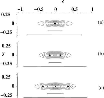
Figure 1: The contours of the electron clouds on the plane $x=0$ for the ${\rm H}$ atom (a), ${\rm H}_{2}^{+}$ ion (b) and ${\rm H}_{3}^{++}$ (c) placed in a magnetic field $B=10^{12}$ G directed along the $z$-axis, $(x,y,z)$ are in a.u. For the ${\rm H}_{2}^{+},{\rm H}_{3}^{++}$-ions the protons are situated on the $z$-line. The values of $2<|z|>$ are shown by bars: the short bars correspond to $B=10^{12}$ G , they are compared with the long bars which correspond to $B=0$ for ${\rm H},{\rm H}_{2}^{+}$ and to $B=10^{10}$ G (near the threshold of existence) for ${\rm H}_{3}^{++}$. It illustrates a shrinking of electronic longitudinal size with magnetic field growth.

The binding energy $E_{\rm b}$ is by definition the difference between the energy of free electron in magnetic field (the Larmor energy) $B$ and the total energy of the atom, $E_{\rm b}=B-E_{\rm T}$. It is known that $E_{\rm b}$ in the weak-field regime is represented by the Taylor expansion in powers of $B^{2}$, while for large $B$ it behaves $\sim(\log^{2}B)$ (see, for example, LL-QM:1977 and discussion in Karnakov:2003 ). Following the above assumption the binding energy depends on the ratio ${{\cal X}}=r_{\rm t}/r_{\rm l}$,

$$E_{\rm b}\ =\ E_{\rm b}({{\cal X}})\ .$$ (5)

It is quite natural to approximate the transverse size $r_{\rm t}\equiv<\rho>$ as follows

$$r_{\rm t}=\frac{r^{0}_{\rm t}}{(1+\alpha_{\rm t}^{2}B^{2})^{1/4}}\bigg{(}\frac{1+a_{\rm t}B^{2}}{1+b_{\rm t}B^{2}}\bigg{)}\ ,$$ (6)

where $r^{0}_{\rm t},\alpha_{\rm t},a_{\rm t},b_{\rm t}$ are parameters, which are found by fitting the calculated expectation values for $<\rho>$. The formula (6) is written in such a way as to reproduce a functionally-correct perturbative expansion of $<\rho>$ at $B=0$ (in powers $B^{2}$) and $r_{\rm t}^{0}=\sqrt{2}a_{\rm B}$, where $a_{\rm B}=1$ a.u. is the Bohr radius. At large $B$ the right-hand side of Eq.(6) behaves as $\sim B^{-1/2}$ simulating the Larmor radius behavior.

Figure 2: ${\rm H}$ atom: the fit of transverse size of the electron cloud $<\rho>$ versus $B$ using Eq.(6). Calculated values are indicated by crosses.

In Fig. 2 one can see that Eq.(6) fits data on $<\rho>$ calculated using the formalism developed in Potekhin:2001 with accuracy better than one percent at $B\gtrsim 10^{9}$ G. The parameters of the fit are given in Table 1. The parameter $\ r^{0}_{\rm t}$ is also found from the fit, it deviates from $\sqrt{2}$ (see above) by $\simeq 8\%$. It reflects the fact that the accuracy provided by formula (6) diminishes as the magnetic field decreases (see the discussion below).

Table 1: The parameters of the fit (6) of the transversal size of the electron clouds of the ${\rm H}$ atom and ${\rm H}_{2}^{+},{\rm H}_{3}^{++},({\rm HeH})^{++},{\rm He}_{2}^{3+}$ ions (in a.u.).

System	$\ r^{0}_{\rm t}$	$\ \alpha_{\rm t}$	$a_{\rm t}$	$b_{\rm t}$
${\rm H}$ atom	1.17533	0.44904	1.20981	1.81098
${\rm H}_{2}^{+}$	0.954427	0.23615	0.376237	0.62194
${\rm H}_{3}^{++}$	0.645875	0.048196	0.00970609	0.0230488
$({\rm HeH})^{++}$	0.174416	0.019657	0.00000030	0.0000003
${\rm He}_{2}^{3+}$	0.200825	0.026449	0.00000150	0.00000148

At first sight, it is a much more complicated task to describe the longitudinal size, $\nobreak{r_{\rm l}\equiv 2<|z|>}$. The approximation we propose to use is

$$r_{\rm l}=\frac{r^{0}_{\rm l}}{1+\alpha_{\rm l}\log(1+\beta_{\rm l}^{2}B^{2}+\gamma_{\rm l}^{2}B^{4})}\bigg{(}\frac{1+a_{\rm l}B^{2}}{1+b_{\rm l}B^{2}}\bigg{)}\ ,$$ (7)

where $r^{0}_{\rm l},\alpha_{\rm l},\beta_{\rm l},\gamma_{\rm l},a_{\rm l},b_{\rm l}$ are parameters, which are found by fitting the calculated expectation values for $2<|z|>$. Formula (7) has the perturbative expansion in powers $B^{2}$, which agrees with perturbation theory results and $r_{\rm l}^{0}=3/2\,a_{B}$, where $a_{\rm B}=1\,$a.u. is the Bohr radius. At large $B$, the right-hand side (7) behaves as $\sim{(\log B)}^{-1}$ as should be in accordance with the qualitative arguments.

Figure 3: ${\rm H}$ atom: the fit of longitudinal size of the electronic cloud $2<|z|>$ versus $B$ using Eq.(7). Calculated values are indicated by crosses.

In Fig. 3 one can see that (7) fits data on $2<|z|>$ obtained in the formalism developed in Potekhin:2001 with accuracy better than 1% at $B\gtrsim 10^{9}$ G. The parameters of the fit are given in Table 2. The parameter $r^{0}_{\rm l}$ is also found from fit. Surprisingly, it deviates from $3/2$ (see above) insignificantly, by $\lesssim 1\,\%$, in contrast to what happened for the parameter $r^{0}_{\rm t}$.

Figure 4: ${\rm H}$ atom: ratio ${\cal X}=\frac{<\rho>}{2<|z|>}$. Calculated values are indicated by crosses.

In Fig. 4 a comparison of the ratio ${{\cal X}}=r_{\rm t}/r_{\rm l}$ (see Eqs. (6)-(7)) with parameters taken from Table 1 with results of calculations is presented. One can clearly see that both data and fitted curves of Figs. 3 and 4 demonstrate a certain irregularity in the range $(5-50)\times 10^{10}$ G. It is a transition region from the Coulomb regime, where the Coulombic forces dominate over magnetic forces to the Landau regime where in the $(x,y)$ plane Coulombic forces become subdominant.

Table 2: The parameters of the fit of the longitudinal size of the electron clouds of ${\rm H}$ atom, ${\rm H}_{2}^{+},{\rm H}_{3}^{++}$ molecular ions as well as $({\rm HeH})^{++},{\rm He}_{2}^{3+}$ using by (7) (in a.u.).

System	$r^{0}_{\rm l}$	$\alpha_{\rm l}$	$\beta_{\rm l}$	$\gamma_{\rm l}$	$a_{\rm l}$	$b_{\rm l}$
${\rm H}$ atom	1.49719	0.179332	0.320252	0.001164	1.07512	1.35162
${\rm H}_{2}^{+}$	1.72041	0.254255	0.141004	0.0004436	0.340131	0.497807
${\rm H}_{3}^{++}$	1.94408	0.279956	0.0191558	0.000008	0.0066712	0.0136894
$({\rm HeH})^{++}$	1.72219	1.155934	0.405312	0.000311	0.131457	0.0600481
${\rm He}_{2}^{3+}$	0.65727	0.228616	0.0011334	0.	0.0000116	0.0000228

Following the assumption (5) let us approximate the binding energy

$$E_{b}=A{{\cal X}}_{\rm l}^{2}+B{{\cal X}}_{\rm l}+C\ ,\ {{\cal X}}_{\rm l}=\log{{\cal X}}\ ,$$ (8)

where $A,B,C$ are parameters, which are found by making fit of the results of calculations of the binding energy. It is worth emphasizing that the parameters of ${{\cal X}}({{\cal X}}_{\rm l})$ are already fixed by the fits (6), (7) of $r_{\rm t},r_{\rm l}$, respectively. The formula (8) agrees with the perturbative expansion in powers $B^{2}$ (at small $B$) and gives a correct asymptotic expansion at large $B$.

Figure 5: ${\rm H}$ atom: the fit of the binding energy using (8). Calculated values are indicated by crosses.

In Fig. 5 it is shown the fit using the formula (8) of the best known results for the binding energies from Kravchenko:1996 combined with those from Potekhin:2001 . The parameters $A,B,C$ are given in Table 3. In the whole range of explored magnetic fields $10^{9}-4.414\times 10^{13}$ G, formula (8) approximates the binding energies with a relative accuracy, which does not exceed few percent and becomes more accurate with growing magnetic field. It is worth mentioning that when the parameter $A=4$ in the approximation (8) its asymptotic coincides with the exact asymptotic (see, e.g., LL-QM:1977 , §112),

$$E_{\rm b}\approx\log^{2}\frac{B}{B_{0}}\ ,\ B\rightarrow\infty\ ,$$ (9)

where $E_{\rm b}$ is in Ry. In fact, the deviation $|A/4-1|$ gives a feeling about the quality of our approximation. Clearly, this estimate is very rough ca. 20 % (see Table III), while a real accuracy of approximating the binding energy is a few percent.

Table 3: The parameters of the fit of the binding energy of the ${\rm H}$ atom, ${\rm H}_{2}^{+},{\rm H}_{3}^{++}$ molecular ions as well as $({\rm HeH})^{++},{\rm He}_{2}^{3+}$ using (8) (all in Ry).

System	$A$	$B$	$C$
${\rm H}$-atom	3.22532	0.53945	1.37932
${\rm H}_{2}^{+}$	8.23442	6.8246	2.99945
${\rm H}_{3}^{++}$	12.8455	20.4849	3.95821
$({\rm HeH})^{++}$	15.7401	6.1134	-5.3756
${\rm He}_{2}^{3+}$	26.2926	32.9181	-0.28129

One of the important characteristics of the magnetic field influence on the ${\rm H}$-atom is the appearance of the quadrupole moment

$$Q\equiv-Q_{zz}=2<z^{2}>-<\rho^{2}>\ .$$ (10)

Recently, the first quantitative study of the quadrupole moment was carried out Potekhin:2001 . The formula (10) suggests immediately the following approximation

$$Q=2r_{\rm l}^{2}(A_{q}-a_{q}{{\cal X}}_{\rm l})-r_{\rm t}^{2}(B_{q}+b_{q}{{\cal X}}_{\rm l})\ ,\ {{\cal X}}_{\rm l}=\log{{\cal X}}\quad,$$ (11)

where $A_{q}=0.325447,a_{q}=0.049432,B_{q}=1.32012,b_{q}=0.955362$ are dimensionless parameters, which are found by fitting the quadrupole moment. The parameters of ${{\cal X}}_{\rm l}$ are already fixed in the fit of parameters $r_{\rm t},r_{\rm l}$ using (6) and (7), respectively. Formula (11) describes correctly the expansion at small and large $B$ (see Ruderman:1971 ; Turbiner:1987 ; Potekhin:2001 ). It fits the results of calculations in Potekhin:2001 with an accuracy of few percents (see Fig. 6).

We made an analysis of the expectation values $<|z|^{n}>$ at $n=2,3,4,5$. It turns out that the calculated expectation values admit a very accurate polynomial approximation in terms of a single expectation value $<|z|>$,

$$<|z|^{n}>\ =\ P_{n}(<|z|>)\ ,$$ (12)

where $P_{n}$ is a $n$-th degree polynomial. It seems natural to assume that (12) holds for any $n$, hence any expectation value is defined by $<|z|>$. This leads to a striking hypothesis that the ground state eigenfunction integrated over $\rho$ can be viewed as a one-parametric probability distribution (!).

Figure 6: ${\rm H}$ atom: the fit of the quadrupole moment using (11). Calculated values (see Potekhin:2001 ) are indicated by crosses.

II The ${\rm H}_{2}^{+}$ molecular ion

In this Section we consider the molecular ion ${\rm H}_{2}^{+}$ in parallel configuration, when the protons are situated along the magnetic line. The form of the electron cloud is illustrated in Fig. 1b for the magnetic field $B=10^{12}$ G. The transversal size of the electron cloud $r_{\rm t}$ shrinks drastically, $\sim B^{-1/2}$, at large magnetic fields, being close to the value of the Larmor radius similarly to what happens for the hydrogen atom. As to the longitudinal size $r_{\rm l}$ it also shrinks but at a much slower rate $\sim{(\log B)}^{-1}$. In particular, the longitudinal size of the electron cloud shrinks in comparison with vanishing magnetic field about five times (see Fig. 1b).

Following the same arguments which were used earlier for the ${\rm H}$ atom, we again assume that the dynamic characteristics of the ${\rm H}_{2}^{+}$ in a magnetic field depend on the expectation values of transversal $(r_{\rm t})$ and longitudinal $(r_{\rm l})$ sizes. The dependence of them on magnetic field is approximated by similar formulas (6)-(7). The binding energy at equilibrium distance between protons depends on the ratio ${{\cal X}}=r_{\rm t}/r_{\rm l}$. Eventually, the binding energy is written in the same form (8) with the same expressions (6) and (7) as is done for ${\rm H}$ atom but with different parameters. For the fit we use the results of recent calculations of the binding energy which were carried out in Turbiner:2003 ; Turbiner:2004 . These parameters of the fit are presented in Tables 1-3 and the fit is illustrated by Figs. 7- 10.

Figure 7: ${\rm H}_{2}^{+}$ ion: a fit of the transverse size of the electron cloud $<\rho>$ using Eq.(6). Calculated values are indicated by crosses.

Figure 8: ${\rm H}_{2}^{+}$ ion: a fit of the longitudinal size of the electron cloud $2<|z|>$ using Eq.(7) (solid curve) and of the equilibrium distance $R_{\rm eq}$ (dashed curve) using Eq.(13). Calculated values are indicated by crosses.

Figure 9: ${\rm H}_{2}^{+}$ ion: the ratio ${{\cal X}}=\frac{<\rho>}{2<|z|>}$. Calculated values are indicated by crosses.

Figure 10: ${\rm H}_{2}^{+}$ ion: the fit of the binding energy using (8). Calculated values are indicated by crosses.

In order to approximate the equilibrium distance $R_{\rm eq}$ we assume that $R_{\rm eq}$ is proportional to the longitudinal distance $r_{\rm l}$ with a small correction in ${{\cal X}}_{\rm l}$

$$R_{\rm eq}=r_{\rm l}(c_{0}+c_{1}{{\cal X}}_{\rm l}+c_{2}{{\cal X}}_{\rm l}^{2})=\frac{r^{0}_{\rm l}}{1+\alpha_{\rm l}\log(1+\beta_{\rm l}B^{2})}\bigg{(}\frac{1+a_{\rm l}B^{2}}{1+b_{\rm l}B^{2}}\bigg{)}(c_{0}+c_{1}{{\cal X}}_{\rm l}+c_{2}{{\cal X}}_{\rm l}^{2})\ ,$$ (13)

where the parameters $c_{0},c_{1},c_{2}$ are found from the fit of the results of calculations of the equilibrium distance which were carried out in Turbiner:2003 ; Turbiner:2004 . The parameters of the fit are given in Table 4. The fit is illustrated in Fig. 8. It is worth mentioning that the parameters $c_{i},\ i=0,1,2$ decrease very fast with $i$ (see Table 4). This can be considered as an indication of adequateness of the approximation formula (13).

Table 4: The dimensionless parameters of the fit (13) of the equilibrium distance (in a.u.) of ${\rm H}_{2}^{+},{\rm H}_{3}^{++}$ and $({\rm HeH})^{++},{\rm He}_{2}^{3+}$ions .

System	$c_{0}$	$c_{1}$	$c_{2}$
${\rm H}_{2}^{+}$	1.37384	0.389879	0.0430844
${\rm H}_{3}^{++}$	4.48200	2.25814	0.380948
$({\rm HeH})^{++}$	4.15754	2.31113	0.409048
${\rm He}_{2}^{3+}$	1.83774	0.51165	0.0626179

Similarly to what happened for ${\rm H}$ atom, the plot of the ratio ${{\cal X}}=r_{\rm t}/r_{\rm l}$ (Fig. 9) reveals a certain irregularity in behavior of the calculation results as well as the fit in the range $(5-50)\times 10^{10}$ G. We assign these irregularities to a transition from the Coulomb to the Landau regime. An overall quality of the fit for the domain $10^{9}-4\times 10^{13}$ G is very high, about 1-2 % except for the above-mentioned region where the accuracy drops to 5-10 %.

Similar to what was done for the ${\rm H}$-atom we carried out a calculation of expectation values $<|z|^{n}>~{}$, $n=2,3,4,5$. It turns out that these expectation values admit very accurate polynomial approximation in terms of the expectation value $<|z|>$ (see (12)). It seems natural to assume that (12) holds for any $n$. This leads to the hypothesis that the ground state eigenfunction integrated over $\rho$ defines a one-parametric distribution similar to what appears for the ${\rm H}$ atom (see previous Section).

III The ${\rm H}_{3}^{++}$ molecular ion

Now we consider the exotic system ${\rm H}_{3}^{++}$ theoretically predicted in Turbiner:1999 , which is made out of three protons situated along the magnetic line and one electron (parallel configuration). This system appears as a quasi-stationary state at $B\gtrsim 10^{10}$ G Turbiner:2004 . The form of the electron cloud for $B=10^{12}$ G is shown in Fig. 1c. It is clearly seen that the transversal size of the electron cloud $r_{\rm t}$ shrinks drastically, $\sim B^{-1/2}$ at large magnetic fields similar to what happens for the hydrogen atom and the ${\rm H}_{2}^{+}$ molecular ion which is of the order of the Larmor radius. As to the longitudinal size $r_{\rm l}$ it also contracts but in much slower rate, $\sim{(\log B)}^{-1}$, at large magnetic fields.

We follow the same idea of approximation as for ${\rm H}$ and ${\rm H}_{2}^{+}$ assuming that the physics is governed by a single parameter ${{\cal X}}=r_{\rm t}/r_{\rm l}$. The same approximation formulas (6) and (7) are used for the transverse ($r_{\rm t}$) and longitudinal ($r_{\rm l}$) sizes, respectively, as it is done for ${\rm H}$-atom and ${\rm H}_{2}^{+}$. Their parameters are found by fitting the results of calculations. The data for $r_{\rm t},r_{\rm l}$ are obtained using a strategy described in Turbiner:2004 . The parameters of the fit are given in Tables 1- 2. The fit of $r_{\rm t}$ and $r_{\rm l}$ is illustrated in Figs. 11- 12. Fig. 13 demonstrates the behavior of the ${\cal X}$. The binding energy $E_{b}$ which is calculated in Turbiner:2004 is approximated using the formula (8) (see Table 3 for parameters of the fit). The fit is illustrated in Fig. 14.

In the same way as it is done for ${\rm H}_{2}^{+}$, we assume that the equilibrium distance between protons are mostly defined by the longitudinal size of the electron cloud (see (7)), which are slightly modified by including the terms depending on ${{\cal X}}_{\rm l}=\log{{\cal X}}$. Finally, the equilibrium distance is approximated by Eq.(13) as was done for ${\rm H}_{2}^{+}$ (see Fig. 12). The parameters of the fit are given in Table 4. It is worth mentioning that the parameters $c_{i},\ i=0,1,2$ decrease very fast with $i$. This might be considered as an indication of adequateness of the approximation formula (13).

In the fit, some irregularities can be seen in the region $(5-50)\times 10^{10}$ G, near the threshold of appearance of the ${\rm H}_{3}^{++}$ ion (see Figs. 11- 14) similarly to those that were observed for the ${\rm H}$-atom and for the ${\rm H}_{2}^{+}$-ion. One of the reasons for these irregularities can be related to highly increased technical difficulties we encountered exploring this region. This could lead to a loss of accuracy. The overall quality of the fit for the range $10^{11}-4.414\times 10^{13}$ G is very high, 1-5 %.

Figure 11: ${\rm H}_{3}^{++}$ ion: the fit of transverse size of the electron cloud $<\rho>$ using Eq.(6). Calculated values are indicated by crosses.

Figure 12: ${\rm H}_{3}^{++}$ ion: the fit of longitudinal size of the electron cloud $2<|z|>$ using Eq.(7) (solid line) and of the equilibrium distance $L_{\rm eq}=2R_{\rm eq}$ using Eq.(13) (dashed line). Calculated values are indicated by crosses.

Figure 13: ${\rm H}_{3}^{++}$ ion: the ratio ${{\cal X}}=\frac{<\rho>}{2<|z|>}$. Calculated values are indicated by crosses.

Figure 14: ${\rm H}_{3}^{++}$ ion: the fit of the binding energy using (8). Only calculated values which are indicated by crosses are used for fitting, while calculated values shown by circles are not taken into account (see text).

Similarly to what was done for the ${\rm H}$ atom and the ${\rm H}_{2}^{+}$ molecular ion, we calculate the expectation values $<|z|^{n}>\ ,\ n=2,3,4,5$ for the ${\rm H}_{3}^{++}$ ion. It turns out that these expectation values admit a very accurate polynomial approximation in terms of the expectation value $<|z|>$, see Eq.(12). It seems natural to assume that (12) holds for any $n$. The ground state eigenfunction integrated over $\rho$ seems to define a certain one-parametric distribution. A similar phenomenon occurs for the ${\rm H}$ atom and the ${\rm H}_{2}^{+}$ molecular ion.

IV The $({\rm HeH})^{++}$ molecular ion

Recently, it was theoretically predicted that the exotic molecular ion $({\rm HeH})^{++}$ can exist for $B\gtrsim 10^{12}$ G Turbiner:2004He . Following the same idea of approximation as it was implemented for the ${\rm H}$ atom and for the ${\rm H}_{2}^{+},{\rm H}_{3}^{++}$ molecular ions, we can construct high-accuracy approximations for the exotic $({\rm HeH})^{++}$ ion. Transversal $(r_{\rm t})$ and longitudinal $(r_{\rm l})$ sizes  of the electron cloud as a function of the magnetic field are approximated by the expressions (6) and (7) (see Figs. 15 and 16). The parameters of the approximations (6)-(7) obtained through fitting the data from Turbiner:2004He are presented in Tables 1-2. In Fig. 17 the ratio ${\cal X}$ is compared with the calculated data from Turbiner:2004He . The fit of the binding energy was performed using the formula (8) (see Fig. 18). The parameters of the fit are presented in Table 3. For the equilibrium distance $R_{\rm eq}$, the approximation (13) is used (see Fig. 16); the parameters are presented in Table 4. The overall quality of the fit for the range $10^{12}-4.414\times 10^{13}$ G is very high, around 1 %.

Figure 15: $({\rm HeH})^{++}$ ion: the fit of the transverse size of the electron cloud $<\rho>$ using Eq.(6). Calculated values are indicated by crosses.

Figure 16: $({\rm HeH})^{++}$ ion: the fit of longitudinal size of the electron cloud $<(z-z_{\rm max})>$ using Eq.(7) (solid line) and the equilibrium distance $R_{\rm eq}$ using Eq.(13) (dashed line). Calculated values are indicated by crosses. All data in a.u.

Figure 17: $({\rm HeH})^{++}$ ion: the ratio ${{\cal X}}=\frac{<\rho>}{<(z-z_{\rm max})>}$. Calculated values are indicated by crosses.

Figure 18: $({\rm HeH})^{++}$ ion: the fit of the binding energy using (8). Calculated values are indicated by crosses.

V ${\rm He}_{2}^{3+}$ molecular ion

Recently, it was theoretically predicted that for $B\gtrsim 100\,$ a.u. the exotic molecular ion ${\rm He}_{2}^{3+}$ can exist Turbiner:2004He . Following the same idea of approximation as for the ${\rm H}$ atom and the ${\rm H}_{2}^{+},{\rm H}_{3}^{++},({\rm HeH})^{++}$ molecular ions (see previous Sections), we would like to construct accurate approximations for the exotic ${\rm He}_{2}^{3+}$ ion. Transversal $(r_{\rm t})$ and longitudinal $(r_{\rm l})$ sizes of the electron cloud as a function of the magnetic field are approximated by the expressions (6) and (7), respectively (see Figs. 19 - 20). The parameters of the approximations (6) and (7) obtained through the fit of the data obtained in Turbiner:2004He are presented in Tables 1- 2, respectively. In Fig. 21 the ratio ${\cal X}$ is compared with the calculated data from Turbiner:2004He . The fit of the binding energy was performed using the formula (8) (see Fig. 22). The parameters of the fit are presented in Table 3. For the equilibrium distance $R_{\rm eq}$ the approximation (13) is used (see Fig. 20) with parameters presented in Table 4.

Some irregularities can be seen in the fit in the region $(2-5)\times 10^{11}$ G, near the threshold of appearance of the ${\rm He}_{2}^{3+}$ ion (see Figs. 19- 22) similar to those which were observed for the ${\rm H}$ atom and for the ${\rm H}_{2}^{+},{\rm H}_{3}^{++}$ ions. The overall quality of the fit for the region $\nobreak{10^{12}-4.414\times 10^{13}}$ G is very high, around 1 %.

Figure 19: ${\rm He}_{2}^{3+}$ ion: the fit of the transverse size of the electron cloud $<\rho>$ using Eq.(6). Only calculated values indicated by crosses, are used for fitting, while the calculated values shown as black squares are not taken into account (see text).

Figure 20: ${\rm He}_{2}^{3+}$ ion: the fit of longitudinal size of the electronic cloud $2<|z|>$ using Eq.(7) (solid line) and of the equilibrium distance $R_{\rm eq}$ using Eq.(13) (dashed line). All data in a.u. Only calculated values which are indicated by crosses are used to make a fit, while calculated values shown by triangles (for longitudinal size data) and by black squares (equilibrium distance data) are not taken into account (see text).

Figure 21: ${\rm He}_{2}^{3+}$ ion: the ratio ${\cal X}=\frac{<\rho>}{2<|z|>}$.

Figure 22: ${\rm He}_{2}^{3+}$ ion: the fit of the binding energy using (8).

VI Conclusion

In this work we presented a phenomenological model of the behavior of different one-electron atomic-molecular systems in a strong magnetic field. The model is based on a surprisingly simple physical idea that the ground state depends on a ratio of transverse to longitudinal size of a system placed in a strong magnetic field only. Since accurate numerical studies in a strong magnetic field are very tedious from a technical point of view a construction of a phenomenological model which provides approximate expressions for basic characteristics of a system for any value of a magnetic field strength can be quite useful for applications.

One of the motivations of the present work is related to the fact that the neutron star atmosphere is characterized by strong magnetic fields, $10^{12}-10^{13}$ G. It seems natural to anticipate a wealth of new physical phenomena there. However, for many years the observational data did not indicate anything unusual, corresponding to the black-body radiation. On 2002, the CHANDRA $X$-ray observatory collected data on an isolated neutron star 1E1207.4-5209 which led to the discovery of two clearly-seen absorption features at $\sim 0.7$ keV and $\sim 1.4$ keV Sanwal:2002 . It is necessary to mention that the XMM-Newton $X$-ray observatory recently confirmed the results of Chandra/ACIS related to absorption features at 0.7 and 1.4 keV Bignami:2003 . We proposed a model of hydrogen atmosphere with main abundance of the exotic ${\rm H}_{3}^{++}$ molecular ion which explains these absorption features assuming that the surface magnetic field is $\sim 5\times 10^{14}$ G Turbiner:2004m . For other neutron stars, observational indications of the existence of absorption lines in their spectra were already foundKerkwijk:2004 ; Vink:2004 . It seems natural to anticipate forthcoming observations of other neutron stars which will likely reveal absorption features. The study presented here can be of certain use in identifying possible absorption features.

VII Acknowledgement

One of us (ABK) is grateful to the Instituto de Ciencias Nucleares, UNAM, where the present work was initiated, for kind hospitality extended to him. This work was supported in part by CONACyT grant 36650-E and DGAPA grant IN124202 (Mexico), and by the RFBR grant 04-02-17263 and a grant of the leading scientific schools 1774.2005.2 (Russia). AVT thanks the University Program FENOMEC (UNAM) for partial financial support.

References

-
(1)
B.B. Kadomtsev and V.S. Kudryavtsev,
Pisma v Zh. Eksp. Ter. Fiz. 13, 15, 61 (1971);
JETP Lett. (Engl. Transl.) 13, 9, 42 (1971) Zh. Eksp. Ter. Fiz. 62, 144 (1972);
Sov. Phys. – JETP 35, 76 (1972) (English Translation) - (2) M. Ruderman, Matter in superstrong magnetic fields: the surface of a neutron star, Phys. Rev. Lett. 27, 1306 (1971); Matter in Superstrong Magnetic Fields, in IAU Symp. 53, Physics of Dense Matter, (ed. by C.J. Hansen, Dordrecht: Reidel, p. 117, 1974)
- (3) A. Turbiner, J.-C. Lopez and U. Solis H., Predicted existence of molecular ions in strong magnetic fields, Pisma v ZhETF 69, 800-805 (1999); JETP Lett. 69, 844-850 (1999) (English Translation), (astro-ph/980929)
- (4) A.V. Turbiner and J.C. Lopez V., The and exotic molecular ions can exist in a strong magnetic field, Preprint ICN-UNAM 04-15, pp.7 (December 2004), (astro-th/0412399), Phys.Rev. A (submitted)
- (5) J.C. Lopez V. and A.V. Turbiner, One-electron linear systems in strong magnetic fields, Phys. Rev. A 62, 022510 (2000), (astro-ph/9911535)
- (6) B.M. Karnakov and V.S. Popov, Hydrogen atom in superstrong magnetic field and the Zeldovich effect, ZhETF 124, 996-1022 (2003), JETP 97, 890-914 (2003) (English Translation)
- (7) R. Garstang, Atoms in high magnetic fields, Rep. Prog. Phys. 40, 105 (1977)
- (8) H. Ruder, G. Wunner, H. Herold and F. Geyer, Atoms in Strong Magnetic Fields, Springer Verlag, Berlin-Heidelberg, 1994
- (9) M.A. Liberman, B. Johansson, Properties of matter in ultrahigh magnetic fields and the structure of the surface of neutron stars, Phys. Usp. 38, 117-136 (1995)
- (10) D. Lai, Matter in Strong Magnetic Fields, Rev. Mod. Phys. 73, 629 (2001), (astro-ph/0009333)
- (11) A.V. Turbiner and J.C. Lopez V., The one-electron molecular systems in a strong magnetic field, Preprint ICN-UNAM 04-17, pp.149 (December 2004), Physics Reports. (submitted)
- (12) A. Potekhin, A. Turbiner, Hydrogen atom in a magnetic field: The quadrupole moment, Phys.Rev. A 63, 065402 (2001), (physics/0101050)
- (13) D. Lai and E. Salpeter, Hydrogen molecules in a superstrong magnetic field: Excitation levels, Phys. Rev. A 53, 152 (1996)
- (14) L. D. Landau and E. M. Lifshitz, Quantum Mechanics, Pergamon Press (Oxford - New York - Toronto - Sydney - Paris - Frankfurt), 1977
- (15) H. Hasegawa and R.W. Howard, Optical absorption spectrum of hydrogenic atoms in a strong magnetic Field, J. Phys. Chem. Sol. 21, 179 (1961)
- (16) Yu. P. Kravchenko, M. A. Liberman and B. Johansson, Exact solution for a hydrogen atom in a magnetic field of arbitrary strength, Phys. Rev. A 54, 287 (1996)
- (17) A.V. Turbiner, On eigenfunctions in quarkonium potential model (perturbation theory and variational method). (In russian), Yad. Fiz. 46, 204 (1987); Sov. J. Nucl. Phys. 46, 125 (1987) (English Translation)
-
(18)
A. Turbiner and J.C. Lopez V.,
in a strong magnetic field: ground state,
Phys. Rev. A 68, 012504 (2003), (astro-ph/0212463) -
(19)
A. Turbiner and J.C. Lopez V.,
in a strong magnetic field: lowest excited states,
Phys. Rev. A 69, 053413 (2004) pp.10, (astro-ph/0310849) -
(20)
A. Turbiner, J.C. López V. and N.L. Guevara,
The exotic ion in a strong magnetic field.
Linear configuration,
Preprint ICN-UNAM 04-07, pp.26, June 2004
Phys. Rev. A (2005) (in print), (astro-ph/0406473) - (21) D. Sanwal, G. G. Pavlov, V. E. Zavlin and M. A. Teter, Discovery of absorption features in the X-ray spectrum of an isolated neutron star, ApJL, 574, L61 (2002), (astro-ph/0206195)
- (22) G.F. Bignami, P.A. Caraveo, A. De Luca and S. Mereghetti, The magnetic field of an isolated neutron star from X-ray cyclotron absorption lines, Nature 423, 725-727 (2003)
- (23) M.H. van Kerkwijk, D. L. Kaplan, M. Durant, S. R. Kulkarni and F. Paerels, A strong, broad absorption feature in the X-ray spectrum of the nearby neutron star RX J1605.3+3249, ApJ, 608, 432-443 (2004), (astro-ph/0311195)
- (24) J. Vink, C. P. de Vries, M. Méndez and F. Verbunt, The continued spectral evolution of the neutron star RX J0720.4+3125, ApJL, 609, L75-L78 (2004), (astro-ph/0404195)
- (25) A.V. Turbiner and J.C. López Vieyra, Hydrogenic molecular atmosphere of a neutron star, Mod. Phys. Lett. A 19, 1919 (2004), (astro-ph/0404290)