The physical origin of the Fresnel drag of light by a moving dielectric medium

Abstract

We present a new derivation of the Fresnel-Fizeau formula for the drag of light by a moving medium using a simple perturbation approach. We focus particulary on the physical origin of the phenomenon and we show that it is very similar to the Doppler-Fizeau effect. We prove that this effect is, in its essential part, independent of the theory of relativity. The possibility of applications in other domains of physics is considered.

I Introduction

It is usual to consider the famous experiment of Fizeau (1851)Fizeau on the drag of light by a uniformly moving medium as one of the crucial experiments which, just as the Michelson-Morley experiment, cannot be correctly understood without profound modification of Newtonian space-time concepts (for a review of Einstein’s relativity as well as a discussion of several experiments the reader is invited to consult Jackson ; Bladel ; Smith ). The result of this experiment which was predicted by FresnelFresnel , in the context of elastic theory, is indeed completely justified by well known arguments due to von Laue (1907) Laue . He deduced the Fresnel-Fizeau result for the light velocity $v$ in a medium, corresponding to a relativistic first order expansion of the Einstein velocity transformation formula:

$$v=\frac{\frac{c}{n_{0}}+v_{e}}{1+\frac{v_{e}}{cn_{0}}}\simeq\frac{c}{n_{0}}+v_{e}\left(1-\frac{1}{n_{0}^{2}}\right)+O\left(\frac{v^{2}}{c^{2}}\right).$$ (1)

Here, $n_{0}$ represents the optical index of refraction of the dielectric medium in its proper frame, and we suppose that the uniform medium motion with velocity $v_{e}$ is parallel to the path of the light and oriented in the same direction of propagation. In the context of electromagnetic theory Minkowsky ; Pauli all derivations of this effect are finally based on the invariance property of the wave operator $\partial_{\mu}\partial^{\mu}[...]$ in a Lorentz transformation. It is easy to write the wave equation $[\partial_{\mathbf{x}^{\prime}}^{2}-\left(n_{0}^{2}/c^{2}\right)\partial_{t^{\prime}}^{2}]\psi=0$ in the co-moving frame R’$\left(\mathbf{x^{\prime}},t^{\prime}\right)$ of the medium in covariant formLeonhardt $[\partial_{\mu}\partial^{\mu}+\left(n_{0}^{2}-1\right)\left(v^{\nu}\partial_{\nu}\right)^{2}]\psi=0$ which is valid in all inertial frames and which for a plane waves, implies the result of Eq. 1. In this calculation we obtain the result $v=c/n_{0}+v_{e}$ if we use the Galilean transformation which proves the insufficiency of Newtonian dynamics.
However, the question of the physical meaning of this phenomenon is not completely clear. This fact is in part due to the existence of a derivation made by Lorentz (1895) Lorentz based on the mixing between the macroscopic Maxwell’s equations and a microscopic electronic oscillator model which is classical in the sense of the Newtonian dynamics. In his derivation Lorentz did not use the relativistic transformation between the two coordinate frames: laboratory and moving medium. Consequently, the relativistic nature of the reasoning does not appear explicitly. Following the point of view of Einstein (1915) Einstein the Lorentz demonstration must contain an implicit hypothesis of relativistic nature, however, this point has not been studied in the literature. Recent developments in optics of moving media Leonhardt ; Wilkens ; Artoni ; Yu allows us to consider this question as an important one to understand the relation between optics, relativity and newtonian dynamics. This constitutes the subject of the present paper. Here, we want to analyze the physical origin of the Fresnel-Fizeau effect. In particular we want to show that this phenomenon is, in its major part, independent of relativistic dynamics.
The paper is organized as follows. In section II we present the generalized Lorentz “microscopic-macroscopic” derivation of the Fresnel formula and the principal defect of this treatment. In section III we show how to derive the Fresnel result in a perturbation approach based on the Lorentz oscillator model and finally in IV we justify this effect independently from all physical assumptions concerning the electronic structure of matter.

II The Lorentz electronic model and its generalization

In this part, we are going to describe the essential contents of the Lorentz model and of its relativistic extension. Let $\boldsymbol{\xi}\left(\boldsymbol{x},t\right)$ be the displacement of an electron from its equilibrium position at rest, written as an explicit function of the atomic position $\boldsymbol{x}$ and of the time $t$. In the continuum approximation we can write the equation of motion for the oscillator as $\partial_{t}^{2}\boldsymbol{\xi}\left(\boldsymbol{x},t\right)+\omega_{0}^{2}\boldsymbol{\xi}\left(\boldsymbol{x},t\right)\simeq-\frac{e}{m}{\mathbf{E}}_{0}e^{-i\left(\omega t-\boldsymbol{k}\cdot\boldsymbol{x}\right)}$ where the supposed harmonic electric incident field appears and where the assumption of small velocity allows us to neglect the magnetic force term. In the case of a non relativistic uniformly moving medium we have

$$\left(\partial_{t}+\boldsymbol{v}_{e}\cdot\boldsymbol{\nabla}\right)^{2}\boldsymbol{\xi}+\omega_{0}^{2}\boldsymbol{\xi}\simeq-\frac{e}{m}\left({\mathbf{E}}_{0}+\frac{\boldsymbol{v}_{e}}{c}\times\boldsymbol{B}_{0}\right)e^{-i\left(\omega t-\boldsymbol{k}\cdot\boldsymbol{x}\right)}$$ (2)

which includes the magnetic field $\boldsymbol{B}=c\boldsymbol{k}\times\boldsymbol{E}/\omega$ of the plane wave and the associated force due to the uniform motion with velocity $\boldsymbol{v}_{e}$. The equation of propagation of the electromagnetic wave in the moving medium has an elementary solution when the velocity of the light and of the medium are parallel. If we refer to a cartesian frame $\boldsymbol{k}=k\hat{\boldsymbol{e}_{x}}$, $\boldsymbol{v}_{e}=v_{e}\hat{\boldsymbol{e}_{x}}$ we have in this case $\boldsymbol{E}=E_{0}e^{-i\left(\omega t-kx\right)}\hat{\boldsymbol{e}}_{y}$, $\boldsymbol{B}=c\frac{k}{\omega}E_{0}e^{-i\left(\omega t-kx\right)}\hat{\boldsymbol{e}}_{z}$ for the electromagnetic field and

$$\boldsymbol{\xi}=-\frac{e}{m}\frac{\boldsymbol{E}_{0}\left(1-\frac{kv_{e}}{\omega}\right)}{\omega_{0}^{2}-\left(\omega-kv_{e}\right)^{2}}e^{-i\left(\omega t-kx\right)}$$ (3)

for the displacement vector parallel to the $y$ axis. The relativistic extension of this model can be obtained directly putting $v_{e}=0$ in Eq. 2 or 3 and using a Lorentz transformation between the moving frame and the laboratory one. We deduce the displacement

$$\boldsymbol{\xi}=-\frac{e}{m}\gamma_{e}\frac{\boldsymbol{E}_{0}\left(1-\frac{kv_{e}}{\omega}\right)}{\omega_{0}^{2}-\gamma_{e}^{2}\left(\omega-kv_{e}\right)^{2}}e^{-i\left(\omega t-kx\right)}$$ (4)

where $\gamma_{e}=1/\sqrt{\left(1-v_{e}^{2}/c^{2}\right)}$. We could alternatively obtain the same result considering the generalization of the Newton dynamics i. e.  by doing the substitutions $m\rightarrow m\gamma_{e}$ and $\omega_{0}\rightarrow\omega_{0}\gamma_{e}^{-1}$ in Eq. 2. The dispersion relation is then completely fixed by the Maxwell equation $\frac{\partial^{2}}{\partial x^{2}}E-\frac{1}{c^{2}}\frac{\partial^{2}}{\partial t^{2}}E=\frac{4\pi}{c^{2}}\frac{\partial}{\partial t}J$, where the current density $J$ is given by the formula $J=-eN\left(\partial_{t}+v_{e}\partial_{x}\right)\xi$ depending on the local number of atoms per unit volume $N$ supposed to be constant. Using $J$ and Eq. 3 or 4 we obtain a dispersion relation $k^{2}=n^{2}\left(\omega\right)\omega^{2}/c^{2}$ where the effective refractive index $n\left(\omega\right)$ depends on the angular frequency $\omega$ and on the velocity $v_{e}$. The more general index obtained using Eq. 4 is defined by the implicit relation

$$n^{2}\left(\omega\right)=1+\gamma_{e}^{2}[n_{0}^{2}\left(\omega^{\prime}\right)-1][1-\frac{n\left(\omega\right)v_{e}}{c}]^{2}.$$ (5)

Here $\omega^{\prime}=\omega\left(1-\frac{nv_{e}}{c}\right)\gamma_{e}$, and $n^{2}_{0}\left(\omega\right)=1+4\pi N_{0}e^{2}/\left(\omega_{0}^{2}-\omega^{2}\right)/m$ is the classical Lorentz index (also called Drude index) which contains the local proper density which is defined in the frame where the medium is immobile by $N_{0}=N\gamma_{e}^{-1}$. These relativistic equations imply directly the correct relativistic formula for the velocity of light in the medium: Writing $n_{0}^{2}-1=(n^{2}-1)(1-v_{e}^{2}/c^{2})/(1-nv_{e}/c)^{2}=(n-v_{e}/c)^{2}/(1-nv_{e}/c)^{2}-1$ we deduce

$$\frac{c}{n_{0}}=\frac{c/n-v_{e}}{1-\frac{v_{e}}{cn}}.$$ (6)

which can be easily transformed into

$$v=\frac{c}{n}=\frac{c/n_{0}\left(\omega^{\prime}\right)+v_{e}}{1+\frac{v_{e}}{cn_{0}\left(\omega^{\prime}\right)}}.$$ (7)

It can be added that by combining these expressions we deduce the explicit formula

$$n^{2}\left(\omega\right)=1+\gamma_{e}^{-2}\frac{[n_{0}^{2}\left(\omega^{\prime}\right)-1]}{[1+\frac{n_{0}\left(\omega^{\prime}\right)v_{e}}{c}]^{2}}.$$ (8)

The non relativistic case can be obtained directly from Eq. 3 or by writting $\gamma_{e}=1$ in Eqs. 5,7. This limit

$$v=\frac{c}{n}\simeq\frac{c}{n_{0}}+v_{e}[1-\frac{1}{n_{0}^{2}}+\omega\frac{d\ln n_{0}}{d\omega}]+O\left(\frac{v_{e}^{2}}{c^{2}}\right)$$ (9)

is the Fresnel-Fizeau formula corrected by a “frequency-dispersion” term due to LorentzLorentz . For our purpose, it is important to note that in the non-relativistic limit of Eq. 5 we can always write the equality

$$\frac{c}{n}=\frac{c-v_{e}}{n^{\prime}}+v_{e}$$ (10)

where $n^{\prime}=n\left(1-v_{e}/c\right)/\left(1-nv_{e}/c\right)$ is the index of refraction defined relatively to the moving medium. We then can see directly that the association of Maxwell’s equation with Newtonian dynamics implies a modification of the intuitive assumption “$c/n_{0}+v_{e}$” used in the old theory of emission. In fact, the problem can be understood in the Newtonian mechanics using the absolute time $t=t^{\prime}$ and the transformation $x=x^{\prime}+v_{e}t^{\prime}$. In the laboratory frame the speed of light, which in vacuum is $c$, becomes $c/n_{0}$ in a medium at rest. In the moving frame the speed of light in vacuum is now $c-v_{e}$Jackson . However, due to invariance of acceleration and resultant force in a galilean transformation we can interpret the presence of the magnetic term in Eq. 2 as a correction to the electric field in the moving frame. This effective electric field affecting the oscillator in the moving frame is then transformed into $E\left(1-nv_{e}/c\right)$. It is this term which essentially implies the existence of the effective optical index $n^{\prime}\neq n_{0}$ and the light speed $\left(c-v_{e}\right)/n^{\prime}$ in the moving frame. It can be observed that naturally Maxwell’s equations are not invariant in a Galilean transformation. The interpretation of $E\left(1-nv_{e}/c\right)$ as an effective electric field is in the context of Newtonian dynamics only formal: This field is introduced as an analogy with the case $v_{e}=0$ only in order to show that $n^{\prime}$ must be different from $n_{0}$.

III Perturbation approach and optical theorem

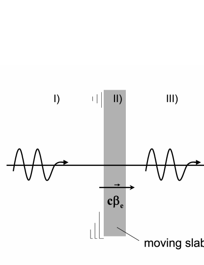
Figure 1: Representation of a linearly polarized electromagnetic plane wave travelling in a moving slab perpendicular to the $x$ axis. The velocity of the slab is $c\beta_{e}$, and the three spatial regions in front, in and after the slab are denoted by 1, 2, and 3, respectively. We have plotted in addition a typical observation point P($x$,0,0).

The difficulty of the preceding model is that the Lorentz derivation does not clarify the meaning of the Fresnel-Fizeau phenomenon. Indeed we justify Eq. 1 using a microscopical model which is in perfect agreement with the principle of relativity. However we observe that at the limit $v_{e}\ll c$ the use of the non relativistic dynamics of Newton (see Eq. 2) gives the same result. More precisely one can see from Eq. 2 that the introduction of the magnetic force $-e\boldsymbol{v}_{e}\times\boldsymbol{B}/c$ in addition to the electric force is already sufficient to account for the Fresnel-Fizeau effect and this even if the classical force formula $\mathbf{F}=m\ddot{\mathbf{x}}(t)$ is conserved. Since the electromagnetic force contains the ratio $v_{e}/c$ and originates from Maxwell’s equations this is already a term of relativistic nature (Einstein used indeed this fact to modify the dynamical laws of NewtonEinstein2 ). The derivation of Lorentz is then based on Newton as well as on Einstein dynamics. It is well know in counterpart that the Doppler-Fizeau effect, which includes the same factor $1-v_{e}/c$, can be understood without introducing Einstein’s relativity. Indeed this effect is just a consequence of the invariance of the phase associated with a plane wave when we apply a Galilean transformation (see Jackson , Chap. 11) as well as a Lorentz transformation. We must then analyze further in detail the interaction of a plane wave with a moving dipole in order to see if the Fresnel phenomenon can be understood independently of the specific Lorentz dynamics.
We consider in this part a different calculation based on a perturbation method and inspired by a derivation of the optical theorem by FeynmanFeynman ; Hulst . Consider a thin slab of thickness $L$ perpendicular to the $x$ axis. Let this slab move along the positive $x$ direction with the constant velocity $v_{e}\boldsymbol{\hat{e}}_{x}$. Let in addition ${\mathbf{E}}_{0}e^{-i\omega\left(t-x/c\right)}$ be the incident electric field of a plane wave which pursues the moving slab (see Fig. 1). Therefore, the electric field after the slab can be formally written as

$${\mathbf{E}}_{\text{after}}={\mathbf{E}}_{0}e^{-i\omega\left(t-\delta t_{v_{e}}-x/c\right)},$$ (11)

where $\delta t_{v_{e}}$ appear as a retardation time produced by the interaction of light with the slab and where all reflections are neglected ($\|{\mathbf{E}}_{\text{after}}\|=\|{\mathbf{E}}_{\text{before}}\|$). For a “motionless” slab (i. e., the case considered by Feynman) we can write the travel time of the light through the slab as $\Delta\tau_{0}=L_{0}/c+\delta t_{0}=n_{0}\cdot L_{0}/c$ and therefore $\delta t_{0}=\left(n_{0}-1\right)\cdot L_{0}/c$ where $L_{0}$ defines the proper length of the slab in the frame where it is at rest. For the general case of a moving slab of reduced length $L=L_{0}\gamma_{e}^{-1}$ we find for the travel time:

$$\Delta\tau_{e}=\frac{\left(L+v_{e}\Delta\tau_{e}\right)}{c}+\delta t_{v_{e}}=n\cdot\frac{\left(L+v_{e}\Delta\tau_{e}\right)}{c}$$ (12)

and therefore the perturbation time is

$$\delta t_{v_{e}}=\frac{\left(n-1\right)L}{\left(c-nv_{e}\right)}.$$ (13)

We can obtain this result more rigorously by using Maxwell’s boundary conditions at the two moving interfaces separating the matter of the slab and the air (see Appendix A).

In order to evaluate the diffracted field which is $\mathbf{E}_{\text{after}}-\mathbf{E}_{\text{before}}$ we can limit our calculation to a first order approximation. Thereby, each dipole of the Lorentz model as discussed above can be considered as being excited directly by the incident electromagnetic wave and where we can neglect all phenomena implying multiple interactions between light and matter. In this limit Eq. 11 reduces to

$${\mathbf{E}}_{\text{after}}={\mathbf{E}}_{0}e^{-i\omega\left(t-x/c\right)}e^{+i\omega\left(n-1\right)\frac{L}{c-nv_{e}}}$$

$$\simeq{\mathbf{E}}_{0}e^{-i\omega\left(t-x/c\right)}\left(1+i\omega\left(n-1\right)\frac{L}{c-nv_{e}}\right).$$ (14)

If the distance between the slab and an observation point is much larger than $L$ we can consider the slab as a 2D continuous distribution of radiating point dipoles. The vector potential ${\mathbf{A}}_{\text{rad}}$ radiated by a relativistically moving point charge $e$ is in according with the Lienard-Wiechert’s formula given by Jackson :

$$\mathbf{A}_{\text{rad}}\left(\mathbf{x},t\right)=e\frac{\mathbf{v}/c}{\left(1-\mathbf{\hat{R}}\cdot\mathbf{\beta}\right)R}|_{ret}.$$ (15)

Here $R=\|\mathbf{x}-\mathbf{x}_{0}\left(t\right)\|$ is the distance separating the observation point $\mathbf{x}$ (denoted by P) and the point charge position located at $\mathbf{x}_{0}\left(t\right)$ at the time $t$; additionally $\boldsymbol{v}\left(t\right)=\dot{\boldsymbol{x}}_{0}\left(t\right)$ is the velocity of the point charge and $\boldsymbol{\hat{R}}\left(t\right)$ is the unit vector $\left(\mathbf{x}-\mathbf{x}_{0}\left(t\right)\right)/R\left(t\right)$. In this formula, in agreement with causality, all point charge variables are evaluated at the retarded time $t_{ret}=t-R\left(t_{ret}\right)/c$.
In the present case the motion of the point charge can be decomposed into a uniform longitudinal component $\mathbf{v}_{e}t$ oriented along the positive $x$ direction and into a transversal oscillating part $\mathbf{\xi}\left(t\right)=\mathbf{\xi}_{0}e^{-i\omega\left(1-\frac{v_{e}}{c}\right)t}$ obeying the condition $\|\dot{\mathbf{\xi}}\left(t\right)\|/c\ll 1$. Owing to this condition we can identify $\left(1-\mathbf{\hat{R}}\cdot\mathbf{v}/c\right)$ with $\left(1-\mathbf{\hat{R}}\cdot\mathbf{v_{e}}/c\right)$. Consequently, in the far-field the contribution of the electron uniform velocity is cancelled by the similar but opposite contribution associated with the nucleus of the atomic dipole: Only the vibrating contribution of the electron survives at a long distance from the diffraction source. If we add the contribution of each dipole of the slab acting on the observation point P at the time $t$ we obtain then the total diffracted vector potential $\mathbf{A}_{\text{diff}}$ produced by the moving medium:

$$\mathbf{A}_{\text{diff}}\left(\mathbf{x},t\right)\simeq-2\pi\gamma_{e}N_{0}Li\omega\frac{e}{c}\left(1-\beta_{e}\right)\mathbf{\xi}_{0}$$

$$\int_{0}^{+\infty}\rho d\rho\frac{e^{-i\omega\left(1-\beta_{e}\right)\left(t-R\left(t_{ret}\right)/c\right)}}{\left(1-\boldsymbol{\hat{R}}\left(t_{ret}\right)\cdot\boldsymbol{v}_{e}/c\right)R\left(t_{ret}\right)},$$ (16)

Here $\rho$ is the radial coordinate in a cylindrical coordinate system using the direction $x$ as a revolution axis, and the quantity $\gamma_{e}N_{0}L2\pi\rho d\rho$ is the number of dipoles contained in the cylindrical volume of length $L$ and of radius varying between $\rho$ and $\rho+d\rho$ if we consider a local dipole density given by $\gamma_{e}N_{0}$. In this formula the retarded distance $R\left(t_{ret}\right)$ is a function of $\rho$ and we have (see the textbook of Jackson Jackson )

$$R\left(t_{ret}\right)=\gamma_{e}^{-1}\left(1-\mathbf{\hat{R}}\left(t_{ret}\right)\cdot\mathbf{v}_{e}/c\right)^{-1}\sqrt{\rho^{2}+\gamma_{e}^{2}\left(x-v_{e}t\right)^{2}}.$$ (17)

This expression shows that the minimum $R_{min}$ is obtained for a point charge on the $x$ axis, and that:

$$R_{min}=\left(x-v_{e}t\right)/\left(1-\beta_{e}\right).$$ (18)

In order to evaluate the integral in Eq. 16 we must use in addition the following relation (see Appendix C):

$$R\left(t_{ret}\right)=\gamma_{e}^{2}\beta_{e}\left(x-v_{e}t\right)+\gamma_{e}\sqrt{\rho^{2}+\gamma^{2}_{e}\left(x-v_{e}t\right)^{2}}$$ (19)

Hence, we obtain the following integral :

$$\mathbf{A}_{\text{diff}}\left(\mathbf{x},t\right)\simeq-2\pi i\omega\gamma_{e}^{2}N_{0}L\frac{e}{c}\left(1-\beta_{e}\right)\mathbf{\xi}_{0}$$

$$\cdot e^{-i\omega\left(1-\beta_{e}\right)\left(t-\gamma_{e}^{2}\beta_{e}\left(x-v_{e}t\right)\right)}$$

$$\cdot\int_{0}^{+\infty}\rho d\rho\frac{e^{i\frac{\omega}{c}\left(1-\beta_{e}\right)\gamma_{e}\sqrt{\rho^{2}+\gamma^{2}_{e}\left(x-v_{e}t\right)^{2}}\}}}{\sqrt{\rho^{2}+\gamma_{e}^{2}\left(x-v_{e}t\right)^{2}}},$$ (20)

where we have used the relations Eq. 17, Eq. 19 in the denominator and in the exponential argument of the right hand side of Eq. 16, respectively. The diffracted field is therefore directly calculable by using the variable $u=\sqrt{\rho^{2}+\gamma_{e}^{2}\left(x-v_{e}t\right)^{2}}$. We obtain the result

$$\mathbf{A}_{\text{diff}}\simeq 2\pi\gamma_{e}LN_{0}\frac{e}{c}\mathbf{\xi}_{0}e^{-i\omega\left(t-x/c\right)}.$$ (21)

The total diffracted electric field $\mathbf{E}_{\text{diff}}$ is obtained using Maxwell’s formula $\mathbf{E}=-\left(1/c\right)\partial_{t}\mathbf{A}$, which gives:

$$\mathbf{E}_{\text{diff}}\simeq 2\pi i\gamma_{e}LN_{0}\omega\frac{e}{c}\mathbf{\xi}_{0}e^{-i\omega\left(t-x/c\right)}.$$ (22)

The final result is given substituting Eq. 4 in Eq. 22 and implies by comparison with Eq. 14

$$n\simeq 1+2\pi N_{0}\gamma_{e}^{2}\frac{e^{2}}{m}\frac{\left(1-\frac{v_{e}}{c}\right)^{2}}{\omega_{0}^{2}-\gamma_{e}^{2}\omega^{2}\left(1-\frac{v_{e}}{c}\right)^{2}}.$$ (23)

This equation constitutes the explicit limit $N_{0}\rightarrow 0$ of Eq. 5 and implies the correct velocity formula Eq. 7 when we neglect terms of $\textrm{O}[N_{0}^{2}]$. It can again be observed that the present calculation can be reproduced in the non relativistic case by neglecting all terms of order $(v_{e}/c)^{2}$.

IV Physical meaning and discussion

The central fact in this reasoning is “the travel condition” given by Eqs. 12,13. Indeed, of the same order in power of $N_{0}$ we can deduce the relation

$$\delta t_{v_{e}}=\gamma_{e}\delta t_{0}\left(1-v_{e}/c\right)$$ (24)

and consequently the condition Eq. 12 reads

$$\Delta\tau_{e}=\frac{L+v_{e}\left(\Delta\tau_{e}-\delta t_{0}\gamma_{e}\right)}{c}+\delta t_{0}\gamma_{e}=n\cdot\frac{\left(L+v_{e}\Delta\tau_{e}\right)}{c}.$$ (25)

If we call $\delta t_{0}$ the time during which the energy contained in a plane of light moving in the positive x direction is absorbed by the slab at rest in the laboratory, $\delta t_{0}\gamma_{e}$ is evidently the enlarged time for the moving case. During the period where this plane of light is absorbed by the slab its energy moves at the velocity $v_{e}$. This fact can be directly deduced of the energy and momentum conservation laws. Indeed, let $M\gamma_{e}v_{e}$ be the momentum of the slab of mass $M$ before the collision and $\epsilon$ the energy of the plane of light, then during the interaction the slab is in a excited state and its energy is now $E^{*}=\epsilon+M\gamma_{e}c^{2}$ and its momentum $P^{*}=\epsilon/c+M\gamma_{e}v_{e}$. The velocity of the excited slab is defined by $w=c^{2}P^{*}/E^{*}$ and we can see that in the approximation $M\rightarrow\infty$ used here $w\simeq v_{e}$ (we neglect the recoil of the slab). During $\delta t_{0}\gamma_{e}$ the slab moves along a path length equal to $v_{e}\delta t_{0}\gamma_{e}$ and thus the travel condition of the plane of energy in the moving slab can be written

$$c\left(\Delta\tau_{e}-\gamma_{e}\delta t_{0}\right)=L+v_{e}\left(\Delta\tau_{e}-\gamma_{e}\delta t_{0}\right),$$ (26)

which is an other form for Eq. 25. Now eliminating directly $\Delta\tau_{e}$ in Eq. 26 give us the velocity $v$ of the wave:

$$v=v_{e}+\frac{c-v_{e}}{1+\frac{c\delta t_{0}}{L}\left(1-\beta_{e}\right)\gamma_{e}},$$ (27)

i. e.

$$v=v_{e}+\frac{c-v_{e}}{1+\left(n_{0}-1\right)\left(1-\beta_{e}\right)\gamma_{e}^{2}},$$ (28)

which depends on the optical index $n_{0}=1+c\delta t_{0}/L_{0}$. After straightforward manipulations this formula becomes

$$v=\frac{c/n_{0}+v_{e}}{1+\frac{v_{e}}{cn_{0}}}$$ (29)

which is the Einstein formula containing the Fresnel result as the limit behavior for small $v_{e}$.
It can be observed that this reasoning is even more natural if we think in term of particles. A photon moving along the axis $x$ and pursuing an atom moving at the velocity $v_{e}$ constitutes a good analogy to understand the Fresnel phenomenon. This analogy is evidently not limited to the special case of the plane wave $e^{i\omega\left(t-x/c\right)}$. If for example we consider a small wave packet which before the interaction with the slab has the form

$$E_{\text{before}}\left(x,t\right)=\int_{\Delta\omega}d\omega a_{\omega}e^{i\left(kx-\omega t\right)},$$ (30)

where $\Delta\omega$ is a small interval centered on $\omega_{m}$, then after the interaction we must have:

$$E_{\text{after}}\left(x,t\right)=\int_{\Delta\omega}d\omega a_{\omega}e^{i\left(kx-\omega[t-\delta t\left(\omega\right)\right)},$$ (31)

where $\delta t\left(\omega\right)$ is given by Eq. 13. After some manipulation we can write these two wave packets in the usual approximative form:

$$E_{\text{before}}\simeq e^{i\left(k_{m}x-\omega_{m}t\right)}\int_{\Delta\omega}d\omega a_{\omega}e^{-i\left(\omega-\omega_{m}\right)[t-\partial k/\partial\omega_{m}x]}$$

$$=e^{i\left(k_{m}x-\omega_{m}t\right)}F\left(t-x/v_{g}\right)$$

$$E_{\text{after}}\simeq e^{i\left(k_{m}x-\omega_{m}[t-\delta t\left(\omega_{m}\right)]\right)}F\left(t-x/v_{g}-\delta t_{g}\right).$$ (32)

Here, $v_{g}=\partial\omega_{m}/\partial k_{m}=c$ is the group velocity of the pulse in vacuum and $\delta t_{g}=\partial\left(\omega_{m}\delta t\left(\omega_{m}\right)\right)/\partial\omega_{m}$ is the perturbation time associated with this group motion. This equation for $F$ possesses the same form as Eq. 11 and then the same analogy which implies Eq. 25 is possible. This can be seen from the fact that we have

$$\delta t\left(\omega\right)=\gamma_{e}\delta t_{0}(\omega^{\prime})\left(1-v_{e}/c\right)$$ (33)

with $\omega^{\prime}=\gamma_{e}\omega(1-v_{e}/c)$. We deduce indeed

$$\delta t_{g}=\gamma_{e}\delta t_{0g}(\omega^{\prime}_{m})\left(1-v_{e}/c\right),$$ (34)

where we have $\delta t_{0g}(\omega^{\prime}_{m})=\partial\left(\omega_{m}\delta t_{0}\left(\omega^{\prime}_{m}\right)\right)/\partial\omega_{m}$ i. e. $\delta t_{0g}(\omega^{\prime}_{m})=\partial\left(\omega^{\prime}_{m}\delta t_{0}\left(\omega^{\prime}_{m}\right)\right)/\partial\omega^{\prime}_{m}$. Since Eq. 33 and Eq. 34 have the same form the Fresnel law must be true for the group velocity.
It is important to remark that all this reasoning conserves its validity if we put $\gamma_{e}=1$ and if we think only in the context of Newtonian dynamics. Since the reasoning with the travel time does not explicitly use the structure of the medium involved (and no more the magnetic force $-e\boldsymbol{v}_{e}\times\boldsymbol{B}/c$) it must be very general and applicable in other topics of physics concerning for example elasticity or sound.
Consider as an illustration the case of a cylindrical wave guide with revolution axis $x$ and of constant length $L$ pursued by a wave packet of sound. We suppose that the scalar wave $\psi$ obeys the equation $[c^{2}\partial^{2}/\partial\mathbf{r}^{2}-\partial^{2}/\partial t^{2}]\psi=0$ where $c$ is the constant sound velocity. The propagative modes in the cylinder considered at rest in the laboratory are characterized by the classical dispersion relation

$$\omega^{2}/c^{2}=\gamma_{n,m}^{2}+k_{x}^{2}$$ (35)

where the cut off wave vector $\gamma_{n,m}$ depend only of the two “quantum” numbers $n,m$ and of the cross section area $A$ of the guide ($\gamma^{2}\sim 1/A$). The group velocity $\partial\omega/\partial k_{x}$ of the wave in the guide is defined by $v_{g}=\left(c^{2}/\omega\right)\sqrt{\omega^{2}/c^{2}-\gamma^{2}}\simeq c[1-\frac{1}{2}c^{2}\gamma^{2}/\omega^{2}]$ and the travel time $\Delta\tau$ by $L/v_{g}\simeq L[1+\frac{1}{2}c^{2}\gamma^{2}/\omega^{2}]/c$ which implies $\delta t_{0}=\frac{1}{2}Lc\gamma^{2}/\omega^{2}$. In the moving case where the cylinder possesses the velocity $v_{e}$ we can directly obtain the condition given by Eq. 25 (with $\gamma_{e}=1$) and then we can deduce the group velocity of the sound in the guide with the formula

$$v=v_{e}+\frac{c-v_{e}}{1+\frac{c\delta t_{0}}{L}\left(1-\beta_{e}\right)}.$$ (36)

This last equation give us the Fresnel result if we put the effective sound index $n_{0}=1+c\delta t_{0}/L$. We can control the self consistency of this calculation by observing that the dispersion relation Eq. 35 allows the definition of a phase index $n_{\text{phase}}=ck/\omega\simeq 1-c^{2}\gamma_{n,m}^{2}/(2\omega^{2})$ which is equivalent to Eq. 25 when $\omega_{0}=0$ and $2\pi N_{0}e^{2}/m=c^{2}\gamma_{n,m}^{2}/2$. This reveals a perfect analogy between the sound wave propagating in a moving cylinder and the light wave propagating in a moving slab. It is then not surprising that the Fresnel result is correct in the two cases.
The principal limitation of our deduction is contained in the assumption expressed above for the slab example: $\|\mathbf{E}_{\text{after}}\|\simeq\|\mathbf{E}_{\text{before}}\|$ i. e. the condition of no reflection supposing the perturbation on the motion of the wave to be small. Nevertheless, the principal origin of the Fresnel effect is justified in our scheme without the use of the Einstein relativity principle.
We can naturally ask if the simple analogy proposed can not be extended to a dense medium i. e. without the approximation of a weak density $N_{0}$ or of a low reflectivity. In order to see that it is indeed true we return to the electromagnetic theory and we suppose an infinite moving medium like the one considered in the second section. In the rest frame of the medium we can define a slab of length $L_{0}$. The unique difference with the section 3 is that now this slab is not bounded by two interfaces separating the atoms from the vacuum but is surrounded by a continuous medium having the same properties and moving at the same velocity $v_{e}$. In the laboratory frame the length of the moving slab is $L=L_{0}\gamma_{e}^{-1}$. We can write the time $\Delta\tau_{e}$ taken by a signal like a wave packet, a wave front or a plane of constant phase to travel through the moving slab:

$$c\Delta\tau_{e}=n\cdot\left(L+v_{e}\Delta\tau_{e}\right).$$ (37)

The optical index $n$ can be the one defined in section 2 for the case of the Drude model but the result is very general. We can now introduce a time $\delta t_{0}$ such that Eq. 25, and consequently Eq. 27, are true by definition. We conclude that this last equation Eq. 27 is equivalent to the relativistic Eq. 29 if, and only if, we define the time $\delta t_{0}$ by the formula

$$\delta t_{0}=\left(n_{0}-1\right)\cdot L_{0}/c.$$ (38)

In other terms we can always use the analogy with a photon pursuing an atom since the general formula Eq. 29 is true whatever the microscopic and Electrodynamics model considered. In this model - based on a retardation effect- the absorbtion time $\delta t_{0}$ is always given by Eq. 38.
This opens new perspectives when we consider the problem of a sound wave propagating in an effective moving medium. Indeed there are several situations where we can develop a deep analogy between the propagation of sound and the propagation of light. This implies that the conclusions obtained for the Fresnel effect for light must to a large part be valid for sound as well. This is in particular true if we consider an effective meta material like the one that is going to be described now:
We consider a system of mirrors as represented in Fig. 2A, at rest in the laboratory. A beam of light propagates along the zigzag trajectory $A_{0},B_{0},A_{1},...,A_{n},B_{n},...$. The length $A_{n}B_{n}$ is given by $\sqrt{(L_{0}^{2}+D^{2})}$ where the distance $L_{0}$ and $D$ are represented on the figure. The time $\Delta\tau_{0}$ spent by a particle of light to move along $A_{n}B_{n}$ is then $\sqrt{(L_{0}^{2}+D^{2})}/c$. We can equivalently define an effective optical index $n_{0}$ such that we have

$$\frac{(L_{0}^{2}+D^{2})}{c^{2}}=\Delta\tau_{0}^{2}=\frac{L_{0}^{2}n_{0}^{2}}{c^{2}}.$$ (39)

This implies

$$n_{0}^{2}=1+\frac{D_{0}^{2}}{L_{0}^{2}}.$$ (40)

We consider now the same problem for a system of mirrors moving with the velocity $v_{e}$. In order to be consistent with relativity we introduce the reduced length $L=L_{0}\gamma_{e}^{-1}$. The beam propagating along the path $A_{0},B_{0},A_{1},...,A_{n},B_{n},...$ must pursue the set of mirrors. We then define the travel time $\Delta\tau_{e}$ along an elementary path $A_{n}B_{n}$ by

$$\frac{((L+v_{e}\Delta\tau_{e})^{2}+D^{2})}{c^{2}}=\Delta\tau_{e}^{2}=\frac{((L+v_{e}\Delta\tau_{e})^{2}n^{2}}{c^{2}},$$ (41)

where $n$ is the effective optical index for the moving medium. From this equation we deduce first $\Delta\tau_{e}=(L/c)n/(1-v_{e}n/c)$ and then

$$n^{2}-1=(n_{0}^{2}-1)\frac{(1-\frac{v_{e}n}{c})^{2}}{(1-(\frac{v_{e}}{c})^{2})}$$ (42)

which finally give us the formula

$$\frac{c}{n}=\frac{c/n_{0}+v_{e}}{1+\frac{v_{e}}{cn_{0}}}$$ (43)

We can again justify the Fresnel formula at the limit $v_{e}/c\ll 1$.

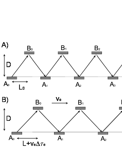
Figure 2: An ideal meta material equivalent to a medium with an effective index. A wave represented by an arrow propagates between the mirrors $A_{0},B_{0},A_{1},...,A_{n},B_{n},...$. A) when the mirrors are at rest in the laboratory the travel time $\delta\tau_{0}=A_{n}B_{n}/c$ is dependent only on the distances $L_{0}$ and $D$. B) When the mirrors move at the velocity $v_{e}$ relatively to the laboratory the travel time $\delta\tau_{e}=A_{n}B_{n}/c$ is affected by the motion and depends on $v_{e}$ as well as on $D$ and $L=L_{0}/\gamma_{e}$.

The simplicity of this model is such that it does not depend on the physical properties of atoms, electrons and photons but only on geometrical parameters. Clearly we can make the same reasoning for a sound wave by putting $\gamma_{e}=1$. This still gives us the Fresnel formula when we neglect terms equal or smaller than $O\left(v_{e}^{2}/c^{2}\right)$. In addition this model allows us to conclude that the essential element justifying the Fresnel-Fizeau result is the emergence of a delay time – a retardation effect– when we consider the propagation of the signal at a microscopic or internal level. The index $n$ which characterizes the macroscopic or external approach is then just a way to define an effective velocity without looking for a causal explanation of the retardation.
The essential message of our analysis is that by taking explicitly into account the physical origin of the delay we can justify the essence of the Fresnel-Fizeau effect in a non relativistic way. The Fresnel-Fizeau effect is then a very general phenomenon. It is a consequence of the conservation of energy and momentum and of the constant value of the wave velocity in vacuum or in the considered medium. The so called travel condition (Eq. 26) which is a combination of these two points can be compared to the usual demonstration for the Doppler effect. In these two cases of light pulses pursuing a moving particle the perturbation time $\delta t_{v_{e}}\simeq\delta t_{0}\left(1-v_{e}/c\right)$ is a manifestation of the Doppler phenomenon. It should be emphasized that the analogy between sound and electromagnetic waves discussed in this article could be compared to the similarities between sound wave and gravitational waves discussed in particular by Unruh. On this subject and some connected discussions concerning the acoustic Aharonov-Bohm effect (that is related to the optical Aharonov-Bohm effect that follows from the Fizeau effect) the reader should consult Unruh1 ; Unruh2 .

V Summary

We have obtain the Fresnel-Fizeau formula using a perturbation method based on the optical theorem and in a more general way by considering the physical origin of the refractive index. The modification of the speed of light in the medium appears then as a result of a retardation effect due to the duration of the interaction or absorbtion of light by the medium, and the Fresnel-Fizeau effect, as a direct consequence of the medium’s flight in front of the light. These facts rely on the same origin as the Doppler-Fizeau effect. We finally have shown that it is not correct to assume, as frequently done in the past, that a coherent and “Newtonian interpretation” of these phenomena would be impossible. On the contrary, the results do not invalidate the derivation of the Fresnel-Fizeau effect based on the principle of relativity but clarify it. We observe indeed than all reasoning is in perfect agreement with the principle of relativity. We must emphasize that even if the Fizeau/Fresnel effect is conceptually divorced from relativity it strongly motivated Einstein’s work (more even than the Michelson and Morley result). The fact that the Fizeau as well as the Michelson-Morley experiment can be justified so easily with special relativity clearly show the advantages of Einstein’s principle to obtain quickly the correct results. Nevertheless, if we look from a dynamical point of view, as it is the case here, this principle plays a role only for effects of order $\mathbf{v}_{e}^{2}/c^{2}$ which however are not necessary to justify the Fresnel formula.

Appendix A

Maxwell’s equations impose the continuity of the electric field on each interface of the slab. More precisely these boundary relations impose: $\mathbf{E}_{\textrm{medium A}}|_{S}=\mathbf{E}_{\textrm{medium B}}|_{S}$ where $S$ is one of the two moving interfaces separating vacuum and matter. Hence we obtain an equality condition between the two phases $\phi_{\textrm{medium A}}$ and $\phi_{\textrm{medium B}}$ valid for all times at the interface. Let $\Phi_{1}=-i\omega\left(t-x/c\right)$ be the phase of the plane wave before the slab. In a similar way let $\Phi_{2}=-i\omega_{2}\left(t-n_{\omega_{2},\beta_{e}}x/c-\delta_{2}\right)$ and $\Phi_{3}=-i\omega_{3}\left(t-x/c-\delta_{3}\right)$ be the phases in the slab and in vacuum after traversing the slab, respectively. In these expressions there appear two retardation constants, $\delta_{2,3}$ and the optical index of the slab. On the first interface denoted by (I-II) we have $x=c\beta_{e}t$ and consequently

$$\omega\left(1-\beta_{e}\right)t=\omega_{2}\left(1-n\left(\omega,\beta_{e}\right)\beta_{e}\right)$$

$$\cdot\left(t-\frac{\delta_{2}}{1-n\left(\omega_{2},\beta_{e}\right)\beta_{e}}\right),$$ (44)

which is valid for each time and possesses the unique solution:

$$\omega_{2}=\omega\frac{1-\beta_{e}}{1-n\left(\omega,\beta_{e}\right)\beta_{e}} ,\delta_{2}=0.$$ (45)

Considering the second interface (II-III) in a similar way we obtain the following conditions

$$\omega_{3}=\omega_{2}\frac{1-n\left(\omega,\beta_{e}\right)\beta_{e}}{1-\beta_{e}}=\omega$$

$$\delta_{3}=L\frac{n\left(\omega,\beta_{e}\right)-1}{c-n\left(\omega,\beta_{e}\right)c\beta_{e}}$$ (46)

where the $2^{nd}$ equality is Eq. 13.

Appendix B

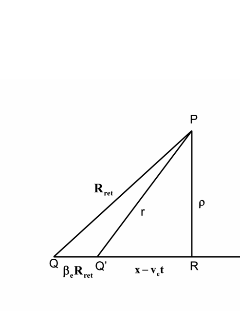
Figure 3: In this figure Q is the position of the particle at the retarded time $t_{ret}$ and P is the observation point at the time $t$. The particle moves uniformly on the the $x$ line QR following the trajectory $v_{e}t$ and Q’ is the position of the particle at the time $t$ separated of P by the distance $r$. In addition, if we call R the projection of P on QR, then $x$ and $\rho$ are the coordinates of the observation point in the plane of the figure.

Using geometrical considerations (see Fig. 3) we can deduce the relation

$$R\left(t_{ret}\right)^{2}=\rho^{2}+\left(\beta_{e}R_{ret}+x-v_{e}t\right)^{2},$$ (47)

which is equivalent after manipulations to the other:

$$\rho^{2}+\gamma_{e}^{2}\left(x-v_{e}t\right)^{2}=\left(1-\beta_{e}^{2}\right)\left(R_{ret}-\beta_{e}\gamma_{e}^{2}\left(x-v_{e}t\right)\right)^{2}.$$ (48)

We can in a second step rewrite this equality as follows:

$$R_{ret}=\gamma_{e}^{2}\beta_{e}\left(x-v_{e}t\right)+\gamma_{e}\sqrt{\rho^{2}+\gamma^{2}_{e}\left(x-v_{e}t\right)^{2}}$$ (49)

which is Eq. 19.

References

- (1) H. Fizeau, C. R. Acad. Sci. (Paris) 33, 349 (1851).
- (2) J. D. Jackson, Classical Electrodynamics, third edition (J. Wiley and Sons, New York, 1999).
- (3) J. van Bladel, Relativity and engineering (Springer-Verlag, Berlin, 1984).
- (4) J. H. Smith, Introduction to special relativity (Benjamin, New York, 1965).
- (5) A. Fresnel, Ann. Chim. Phys. 9, 57 (1818).
- (6) H. von Laue, Ann. Phys. (Leipzig) 23, 989 (1907).
- (7) H. Minkowsky, Nachr. d. K. Ges. d. Wiss. Zu Gott., Math. -Phys. Kl. 53 (1908).
- (8) W. Pauli, Theory of relativity (Pergamon press, London, 1958).
- (9) H. A. Lorentz, The theory of electrons and its application to the phenomena of light and radiant heat, 2nd edn. , chapter 5 (B. G. Teubner, Stutters, 1916).
- (10) A. Einstein, Über die spezielle und die allgemeine relativitätstheorie gemeinverstänlich (Vieweg, Brunswick, 1917).
- (11) U. Leonhardt and P. Piwinicki, Phys. Rev. A60, 4301 (1999); J. Fiurazek, U. Leonhardt and R. Parentani, Phys. Rev. A65, 011802 (2002); U. Leonhardt and P. Piwinicki, Phys. Rev. Lett. 84, 822 (2000); U. Leonhardt, Phys. Rev. A62, 012111 (2000); U. Leonhardt and P. Ohberg, Phys. Rev. A67, 053616 (2003).
- (12) M. Wilkens, Phys. Rev. Lett. 72, 5 (1994); H. Wei, R. Han and X. Wei, ibid. 75 2071, (1995); G. Spavieri, ibid. 82, 3932 (1999).
- (13) I. Carusotto, M. Artoni, G. C. La Rocca, and F. Bassani, Phys. Rev. Lett. 86, 2549 (2001); M. Artoni and I. Carusotto, Phys. Rev. A68, 011602 (2003); I. Carusotto, M. Artoni, G. C. La Rocca, and F. Bassani, Phys. Rev. A68, 063819 (2003).
- (14) D. Strekalov, A. B. Matsko. N. Yu. and L. Maleki, Phys. Rev. Lett. 93, 023601 (2004).
- (15) A. Einstein, Ann. Phys. (Leipzig) 17, 891 (1905).
- (16) R. P. Feynman, R. B. Leighton and M. L. Sands, The Feynman Lectures on Physics, chapters 30-31 (Addison-Wesley, Massachusetts, 1963).
- (17) H. C. van de Hulst, Light scattering by small particles, chapter 4 (John Wiley and Sons Inc. , New York, 1957).
- (18) W. G. Unruh, Phys. Rev. Lett. 46, 1351 (1981); M. Visser, Class. Quant. Grav. 15, 1767 (1998).
- (19) S. E. P. Bergliaffa, K. Hibberd, M. Stone, and M. Visser, Physica D 191, 121 (2004); P. Roux, J. de Rosny, M. Tanter, and M. Fink, Phys. Rev. Lett. 79, 3170 (1997).