Self-similarities in the frequency-amplitude space of a loss-modulated CO₂ laser

Abstract

We show the standard two-level continuous-time model of loss-modulated CO₂ lasers to display the same regular network of self-similar stability islands known so far to be typically present only in discrete-time models based on mappings. For class B laser models our results suggest that, more than just convenient surrogates, discrete mappings in fact could be isomorphic to continuous flows.

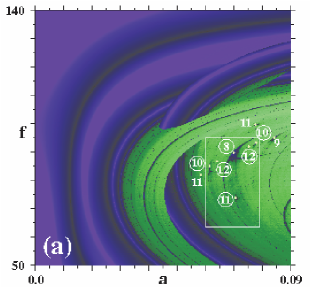
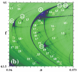
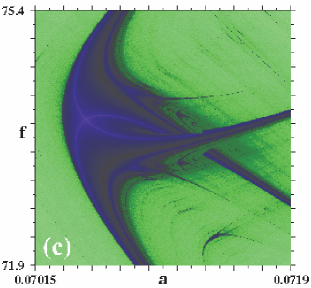
Figure 1: (Color online) Structure of the frequency-amplitude phase-diagram of the laser showing a regular network of stability islands (a) Global view, (b) Zoom of the box in (a). Numbers indicate the main period of each stability island; (c) Magnification of the period-11 stability island (indicated in (b) by the encircled 11), displaying the generic shape of all stability islands fest . Color intensities are proportional to Lyapunov exponents: blue for negative exponents (periodic oscillations), black for zero and green for positive exponents (chaotic oscillations). Frequencies are in kHz.

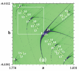
Figure 2: (Color online) Structure of the parameter space of the Hénon map. (a) The organization of shrimps here coincides with that of the laser (compare with Fig. 1b). The fine structure observed around period-8 here reproduces the laser period-8 sequence along the curve passing by the encircled numbers in Fig. 1b; (b) Magnification of the box in (a); (c) Magnification of the box in (b). Numbers indicate the main period of each stability island. Points mark windows, not doubly superstable crossings. Download ALL figures high-res PDF: http://www.if.ufrgs.br/$\sim$jgallas/jg_papers.html

Lasers with modulated parameters are arguably among the simplest and most accessible laser systems of interest for applications in science and engineering and for theoretical investigations. The intrinsic interest in practical applications and in the nonlinear dynamics of modulated lasers has spurred a wide range of studies after the remarkably influential work of Arecchi et al. arecchi82 reporting the first measurement of subharmonic bifurcations, multistability, and chaotic behavior in a Q-switched CO₂ laser. Since then, CO₂ lasers have been fruitfully exploited in many situations. Recent applications include studies of stochastic bifurcations in modulated CO₂ laser lora2004 , multistability induced by periodic modulations chiz_pre64 . Rich nonlinear response of CO₂ lasers with current modulation and cavity detuning pisa-josaB , and self-focusing effects in nematic liquid crystals brugioni .

In the last 20 years the CO₂ laser was extensively studied theoretically, numerically and experimentally gilmore ; solari ; tredicce ; dangoisse , but focusing mainly on the characterization of dynamical behaviors in phase-space for specific parameters. While a detailed description of phase-space dynamics is already available in the literature gilmore ; asy ; hilborn ; strogatz , no equivalent description exists for the parameter space, except for works by Goswami gos_pla190 who investigated analytically the first few period-doubling bifurcations for the Toda model of the CO₂ laser toda .

The present Letter reports an investigation of the parameter space of a paradigmatic model of class B lasers, the CO₂ laser. More specifically, we study a popular two-level model of a CO₂ laser with modulated losses, focusing on the global stability of the laser with respect to the modulation, not the intensity. The remarkable discovery reported here is that stability islands of the continuous-time laser model emerge organized in a very regular network of self-similar structures called shrimps jason , illustrated in Figs. 1 and 2, and previously known to exist only in the parameter space of discrete-time dynamical systems jason ; fest ; nusse ; brian . Thus far, all attempts to uncover shrimps in flows, i.e. in continuous-time dynamical systems modeled with sets of differential equations, have failed to produce them potsdam .

The single-mode dynamics of the loss-modulated CO₂ laser involves two coupled degrees of freedom and a time-dependent parameter which we write, as usual chiz_pre64 ; gilmore ; tredicce ,

$$\centering\frac{du}{dt}\@add@centering = \frac{1}{\tau}\,(z-k)u,$$ (1a)

$$\frac{dz}{dt} = (z_{0}-z)\gamma-uz.$$ (1b)

Here, $u$ is proportional to the radiation density, $z$ and $z_{0}$ are the gain and unsaturated gain in the medium, respectively, $\tau$ denotes the transit time of the light in the laser cavity, $\gamma$ is the gain decay rate, and $k\equiv k(t)$ represents the total cavity losses. The losses are modulated periodically as follows,

$$k(t)=k_{0}(1+a\cos 2\pi ft),$$ (2)

where $k_{0}$ is the constant part of the losses and $a$ and $f$, the amplitude and frequency of the modulation, are the main bifurcation parameters. The remaining parameters are fixed at $\tau=3.5\times 10^{-9}$ s, $\gamma=1.978\times 10^{5}$ s^-1, $z_{0}=0.175$ and $k_{0}=0.1731$. These are realistic values, used in recent theoretical and experimental investigations chiz_pre64 . Integrations were done using the standard fourth-order Runge-Kutta scheme with fixed time-step, equal to $h=4\times 10^{-8}$. Phase diagrams in $a\times f$ space are obtained by computing Lyapunov exponents for a mesh of $600\times 600$ equally spaced parameters. Starting from an arbitrary initial condition, we “followed the attractor” that is, after increasing parameters we initiated iterations using the last obtained values as the new initial conditions. The largest exponents were codified into a bitmap with a continuous color scale ranging from the maximum positive (green) to maximum negative (blue) exponents. Zero exponents were codified in black. One of the exponents is always zero since it is simply related to the time evolution. Three illustrative bitmaps for the laser model are shown in Fig. 1.

Figure 1a displays a global view of the parameter space. The most prominent features, the broad curved structures in Fig. 1a, show that the parameter space of the laser model above, Eqs. (1a-b), agrees qualitatively quite well with the description of Goswami gos_pla190 for the Toda model of the CO₂ laser. For the parameters chosen, the relaxation frequency of our laser model is $50$ kHz. From Fig. 1a it is possible to see that there is a minimum amplitude threshold $a$ beyond which subharmonic bifurcations start to occur, corresponding to about $100$ kHz, the harmonic of the relaxation frequency. In addition, for certain parameter values new stability domains are created by saddle-node bifurcations, each of them undergoing then its own cascade of period doublings. So, in certain parameter ranges more than one stable mode coexist, giving rise to generalized multistability. This feature may be recognized in Fig. 1 from the apparent sudden discontinuities in the coloring, due only to the impossibility of plotting two distinct colors in the same place.

Figure 3: Comparison of return maps. Left column: Laser return maps for period-8 and its pair of doublings. Parameters are: (a) $(a,f)=(0.06984$, $89.8)$, period 8, (b) $(0.07138$, $90.47)$, period 16, (c) $(0.06902$, $87.43)$, period 16. Frequencies are in kHz. Right column: Hénon return maps for period-8 and its doublings seen at the center of Fig. 2a. Parameters are: (d) $(a,b)=(1.8087$, $-0.02514)$, period 8, (e) $(1.80395$, $-0.0257)$, period 16, (f) $(1.80642$, $-0.02356)$, period 16.

The most interesting feature in Fig. 1a is the remarkably regular structuring which appears in the region containing the box, shown magnified in Fig. 1b. This figure shows that embedded in the wide domain of parameters leading to chaotic laser oscillations there is a regular structuring of self-similar parameter windows, shrimps, containing cascades of stable periodic oscillations, the main period of a few of the larger shrimps indicated by the number near to them. The period-11 shrimp seen in Fig. 1b is shown magnified in Fig. 1c. Starting from the main period-11 body, it displays two distinct doubling cascades as well as an infinite number of additional period-doubling cascades, as thoroughly described for discrete-time systems in Refs. jason ; fest .

Figure 4: Time evolution of the laser intensity $u(t)$ for the large period-8 structure in Fig. 1b, plotted in (a) logarithmic scale, (b) linear scale. Here $T=1/(89.8\hbox{ kHz})$ is the period of the modulation.

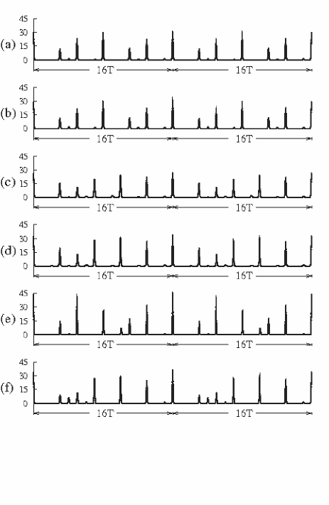
Figure 5: Predicted signal intensity for the six period-16 stability islands labeled A, B, …F, in Fig. 1b. Signals (a) and (b), at points A and B, are period-8 doublings. All other signals are from islands which begin with period-16. Note that signals look very similar, despite the fact that they originate from very distinct regions of the parameter space. Parameters $(a,f)$ are: (a) $A=(0.06902$, $87.43)$, (b) $B=(0.07138$, $90.47)$, (c) $C=(0.063715$, $92.15)$, (d) $D=(0.062255$, $75.735)$, (e) $E=(0.0749617$, $67.3281)$, (f) $F=(0.073666$, $83.359)$. Note that $T\equiv 1/f$ is slightly different for each signal.

The computation of bitmaps for the laser model is very computer demanding. To alleviate this problem and to manifest the isomorphism between flows and maps, we display the generic fine and hyperfine structure of stability islands typically present in multidimensional systems using the two-parameter Hénon map as a paradigm:

$$x_{t+1}=a-x_{t}^{2}+b\,y_{t},\qquad y_{t+1}=x_{t}.$$ (3)

The nonlinearity parameter $a$ (forcing) represents the bifurcation or control parameter. The damping parameter $b$ varies between $-1\leq b\leq 1$, with $b=1$ representing the conservative limit and $b=0$ the limit of strong damping. While for $b=0$ there exists just a single chaotic attractor over a wide range of the parameter $a$, several periodic and chaotic attractors coexist when $b\neq 0$.

Since all these attractors evolve in the same generic manner, we consider here the strongly dissipative limit, focusing on slightly negative values of $b$. In this domain, Pando et al. pando found that a much more sophisticated four-level model of the CO₂ laser with modulated losses behaves qualitatively similar to the Hénon map. The CO₂ laser dynamics, as of any class B laser, is characterized by a time-delay between the intensity and the population inversion, a fact that nicely matches the delayed character of the Hénon map when written as a one-dimensional recurrence relation.

Figure 2 shows how regularly shrimps organize themselves along very specific directions in parameter space. The ordering along the main diagonal of Fig. 2a is the same found for the laser, in Fig. 1a, along the direction containing the encircled periods. Analogously, the secondary diagonal in Fig. 2a displays the same ordering that the parabolic arc in the middle of Fig. 1c.

The laser-Hénon agreement in parameter space permeates also to the phase space as corroborated by Fig. 3, comparing return maps for the laser (on the left column) with those for the Hénon map (right column). The laser return maps were constructed using the sequence $u_{\ell}(t)$, $\ell=1,2,3,\dots$ of relative maxima of $u(t)$. As it is easy to see, both sets of return maps agree remarkably well elsewhere .

How easy is to detect experimentally the regular structuring reported here? Figure 4 illustrates a representative laser signal in two scales. Although waveforms and underlying periodicities are easy to recognize in logarithmic scale, their experimental detection may become strenuous, particularly as the period increases. For instance, contemplating the six period-16 stability islands in Fig. 1b, two of them arising from period-8 via saddle-node bifurcations, one may ask what sort of differences should be expected in their measurement. The answer is depicted in Fig. 5. In a real experimental setup, the difficulties to surmount are mainly to access narrow high-period windows, and to have a wide enough detection range. Modulated losses are usually obtained with an intracavity polarizer and an electro-optical modulator. Recent progress in low-voltage electro-optical modulators have considerably improved their performances eom . To detect large and small peaks simultaneously one can use a logarithmic preamplifier lefranc . Thus, detection and discrimination of the laser signals in Fig. 5 is experimentally feasible with existing technology.

To uncover isomorphisms between continuous-time (flows) and discrete-time (maps) in dynamical systems is an important event from a physical and dynamical point of view and immediately raises interesting questions. For instance, is an isomorphism to be expected also for more refined laser models such that, e.g., of Ciofini et al. politi_model , involving two rate-equations derived for a single-mode CO₂ laser using center manifold theory for a four-levels model meucci ? Their model is interesting because, as they say, it agrees well with experiments. Do networks of shrimps exist for the laser model proposed very recently by Meucci et al. meucci2004 . Do they exist for other laser models too? Is it possible to find them in the parameter space of the laser parameters, not modulation? In autonomous systems? Which laser system presents more restricted amplitude variations, making life easier for experimentalists? What sort of mechanism generates shrimps in differential equations? How are basins of attraction entangled in multistable domains where self-similar structures are abundant rech ? We will report on this elsewhere.

We thank P. Glorieux for a critical reading of the manuscript and helpful suggestions. CB thanks Conselho Nacional de Desenvolvimento Científico e Tecnológico (CNPq), Brazil, for a doctoral fellowship. JACG thanks CNPq for a senior research fellowship and the Université de Lille for a “Professeur invité” fellowship.

References

- (1) F.T. Arecchi, R. Meucci, G. Puccioni, and J. Tredicce, Phys. Rev. Lett. 49, 1217 (1982).
- (2) L. Billings, I.B. Schwartz, D.S. Morgan, E.M. Bollt, R. Meucci and E. Allaria, Phys. Rev. E 70, 26220 (2004).
- (3) V.N. Chizhevsky, Phys. Rev. E 64, 036223 (2001).
- (4) A.N. Pisarchik and B.F. Kuntsevich, J. Opt. B: Quantum Semiclass. Opt. 3, 363 (2001).
- (5) S. Brugioni and R. Meucci, Eur. J. Phys. D, 28, 277 (2004).
- (6) R. Gilmore and M. Lefranc, The Topology of Chaos, Alice in Stretch and Squeezeland, (Wiley, New York, 2002); R. Gilmore, Rev. Mod. Phys. 70, 1455 (1998).
- (7) H.G. Solari, E. Eschenazi, R. Gilmore, and J.R. Tredicce, Opt. Commun. 64, 49 (1987).
- (8) J.R. Tredicce, F.T. Arecchi, G.P. Puccioni, A. Poggi, and W. Gadomski, Phys. Rev. A 34, 2073 (1986).
- (9) D. Dangoisse, P. Glorieux, and D. Hennequin, Phys. Rev. A 36, 4775 (1987); Phys. Rev. Lett. 57, 2657 (1986).
- (10) E. Ott, Chaos in Dynamical Systems, 2nd edition, (Cambridge University Press, Cambrigde, 2002). K.T. Alligood, T.D. Sauer and J.A. Yorke, Chaos: an Introduction to Dynamical Systems, (Springer, New York, 1997);
- (11) R.C. Hilborn, Chaos and Nonlinear Dynamics: An Introduction for Scientists and Engineers, 2nd edition, (Oxford University Press, Oxford, 2000).
- (12) S.H. Strogatz, Nonlinear Dynamics and Chaos: With Applications to Physics, Biology, Chemistry and Engineering, (Perseus, Cambridge MA, 1994).
- (13) B.K. Goswami, Phys. Lett. A 190, 279 (1994); Phys. Lett. A 245, 97 (1998).
- (14) G.L. Oppo and A. Politi, Z. Phys. B 59, 111 (1985).
- (15) J.A.C. Gallas, Phys. Rev. Lett. 70, 2714 (1993); Physica A 202, 196 (1994).
- (16) J.A.C. Gallas, Appl. Phys. B, 60, S-203 (1995), special supplement, Festschrift Herbert Walther.
- (17) J.A.C. Gallas and H.E. Nusse, J. Economic Behavior and Organization 29, 447 (1996).
- (18) B.R. Hunt, J.A.C. Gallas, C. Grebogi, J.A. Yorke and H. Koçak, Physica D 129, 35 (1999).
- (19) M. Thiel, M.C. Romano, W. von Bloh, and J. Kurths kindly informed us to have recently found shrimps while computing recurrence plots.
- (20) C.L. Pando, G.A. Luna Acosta, R. Meucci and M. Ciofini, Phys. Lett. A 199, 191 (1995).
- (21) A prototypical map particularly suited to investigate analytically the inner structure of stability islands is the canonical quartic map , introduced in Ref. jason and discussed at length in Refs. fest ; brian .
- (22) V. Berger, N. Vodjdani, D. Delacourt and J.P. Schnell, Appl. Phys. Lett. 68, 1904 (1996).
- (23) M. Lefranc, D. Hennequin, and P. Glorieux, Phys. Lett. A 163, 269 (1992).
- (24) M. Ciofini, A. Politi, and R. Meucci, Phys. Rev. A 48, 605 (1993).
- (25) C.L. Pando, R. Meucci, M. Ciofini, and F.T. Arecchi, Chaos 3, 279 (1993).
- (26) R. Meucci, D. Cinotti, E. Allaria, L. Billings, I. Triandaf, D. Morgan and I.B. Schwartz, Physica D 189, 70 (2004).
- (27) P.C. Rech, M.W. Beims and J.A.C. Gallas, Phys. Rev. E 71, 017202 (2005).