A New Technique for Finding Needles in Haystacks:
A Geometric Approach to Distinguishing Between a New Source and Random Fluctuations

Abstract

We propose a new test statistic based on a score process for determining the statistical significance of a putative signal that may be a small perturbation to a noisy experimental background. We derive the reference distribution for this score test statistic; it has an elegant geometrical interpretation as well as broad applicability. We illustrate the technique in the context of a model problem from high-energy particle physics. Monte Carlo experimental results confirm that the score test results in a significantly improved rate of signal detection.

One of the fundamental problems in the analysis of experimental data is determining the statistical significance of a putative signal. Such a problem can be cast in terms of classical “hypothesis testing”, where a null hypothesis $\mathcal{H}_{0}$ describes the background and an alternative hypothesis $\mathcal{H}_{1}$ characterizes the signal together with the background. A test statistic (a function of the data) is used to decide whether to reject $\mathcal{H}_{0}$ and conclude that a signal is present.

The hypothesis test concludes that a signal is present whenever the test statistic falls in a critical region $W$. One is interested in the probability that a signal is found under two scenarios. First, when the null hypothesis $\mathcal{H}_{0}$ is true, the significance level $\alpha$ is the probability of incorrectly concluding that a signal is present. Second, when the alternative $\mathcal{H}_{1}$ is true, the power of the test is the probability that the signal is found. The goal is to construct a test statistic whose asymptotic distribution (reference distribution under $\mathcal{H}_{0}$ for large sample size) can be calibrated accurately and that the associated test has high power at a fixed significance level, such as $\alpha=0.01$.

When the two hypotheses are distinct, a powerful technique based on the likelihood ratio test (LRT) is often used. Suppose $p(x;{\mbox{\boldmath$\theta$}})$ is a probability density function for a measurement $x$ with a parameter vector ${\mbox{\boldmath$\theta$}}\in\Theta\subset\mathcal{R}^{d}$. The joint probability density function evaluated with $n$ measurements ${\bf X}$ for an unknown $\theta$ is the likelihood function [1] $L({\mbox{\boldmath$\theta$}}|{\bf X})$. An effective approach to the problem of choosing between $\mathcal{H}_{0}$ [corresponding likelihood $L({\mbox{\boldmath$\theta$}}_{0}|{\bf X})$] and $\mathcal{H}_{1}$ [with a likelihood $L({\mbox{\boldmath$\theta$}}_{1}|{\bf X})$] for explaining the data is to consider the LRT statistic: $\Lambda=L(\widehat{{\mbox{\boldmath$\theta$}}}_{0}|{\bf X})/L(\widehat{{\mbox{\boldmath$\theta$}}}_{1}|{\bf X})$, where $\widehat{{\mbox{\boldmath$\theta$}}}$ is the value of $\theta$ that maximizes $L({\mbox{\boldmath$\theta$}}|{\bf X})$ [1–3]. To employ the LRT, the parsimonious model under $\mathcal{H}_{0}$ (with $s_{0}$ parameters) must be nested within the more complicated alternative model under $\mathcal{H}_{1}$ (with $s_{1}$ parameters). For simple models, under regularity conditions, $2\,\log(\Lambda)$ is distributed as the $\chi^{2}$ distribution with $(s_{1}-s_{0})$ degrees of freedom under $\mathcal{H}_{0}$ [1].

When the alternative hypothesis corresponds to a signal which is a perturbation of the background, regularity conditions required for this asymptotic theory are violated, since (a) some of the parameters under $\mathcal{H}_{0}$ are on the boundaries of their region of support and (b) different parameter values give rise to the same null model. As a result, the LRT has lacked an analytically tractable reference distribution required to calibrate a test statistic. Such a difficulty occurs in many practical applications, for example, when testing for a new particle resonance of unknown production cross section as the signal strength must be nonnegative. Hence, the LRT must be employed cautiously; however, it has been employed in several problems of practical importance where certain required regularity conditions are violated [2]. An inappropriate application of the LRT statistics can lead to incorrect scientific conclusions [4,5].

In light of the above difficulties with the LRT, a $\chi^{2}$ goodness-of-fit test is commonly employed. However, it typically has less power than might be hoped for as it does not take into account information about the anticipated form of the signal. We propose a new test statistic based on a score process to detect the presence of a signal and present its reference distribution. This score statistic is closely related to the LRT for sufficiently large sample size.

Consider the model

$$p(x;\eta,{\mbox{\boldmath$\theta$}})=(1-\eta)\,f(x)+\eta\,\psi(x;{\mbox{\boldmath$\theta$}}),$$

where $f(x)$ is a specified null density and $\psi(x,{\mbox{\boldmath$\theta$}})$ is a perturbation density. The parameter vector $\theta$ is the “location” of the perturbation, and $\eta\in[0,1]$ measures the “strength of the perturbation”. The null hypothesis of no signal ($\mathcal{H}_{0}\!:\eta=0$) implies that $p(x;0,{\mbox{\boldmath$\theta$}})=f(x)$ for all $x$ independently of $\theta$; hence we are in the scenario (b). In searching for a new particle resonance, for example, one measures the frequency of events as a function of energy $E$, modeling it by $p(E;\eta,E_{0})$, where $f(E)$ characterizes the background density and $\psi(E;E_{0})=[\Gamma/(2\,\pi)][(E-E_{0})^{2}+(\Gamma/2)^{2}]^{-1}$ is the Cauchy (Breit-Wigner) density describing a resonance centered on $E_{0}$ with full width at half-maximum $\Gamma$. In this scenario, $\eta=0$ under $\mathcal{H}_{0}$ and hence the asymptotic distribution of $2\,\log(\Lambda)$ under $\mathcal{H}_{0}$ does not have an asymptotic $\chi^{2}$ distribution. The asymptotic reference distribution is not analytically tractable, and hence it is not possible to employ its measured value for valid statistical inference.

A key obstacle to detecting the signal is finding the tail probability. We provide an asymptotic solution to this problem via a geometric formula (see Eq. [3]). The relative improvement of the score test over the $\chi^{2}$ goodness-of-fit test is particularly salient when the signal is hard to detect (see Fig. 4). The development of the reference distribution and a flexible computational method will enable making probabilistic statements to solving some of the fundamental problems arising in many experimental physics.

Pilla and Loader [6] have developed a general theory and a computationally flexible method to determine the asymptotic reference distribution of a test statistic under $\mathcal{H}_{0}$. Their method is based on the “score process”, indexed by the parameter vector $\theta$ and defined as ${\rm S}({\mbox{\boldmath$\theta$}}):=\partial\,\log[\prod_{i=1}^{n}p(E_{i};\eta,{\mbox{\boldmath$\theta$}})]/\partial\eta\big{|}_{\eta=0}$ for a given data ${\mathbf{E}}=(E_{1},\ldots,E_{n})$. Under $\mathcal{H}_{0}$, the expectation of ${\rm S}({\mbox{\boldmath$\theta$}})$ is $0$ for all $\theta$, while under $\mathcal{H}_{1}$ it has a peak at the true value of $\theta$. Hence, the statistic ${\rm S}({\mbox{\boldmath$\theta$}})$ is sensitive to the signal of interest. The random variability of ${\rm S}({\mbox{\boldmath$\theta$}})$ can exhibit significant dependence on the parameter vector $\theta$, hence we consider the normalized score process defined as

$${\rm S}^{\star}({\mbox{\boldmath$\theta$}}) := \frac{{\rm S}({\mbox{\boldmath$\theta$}})}{\sqrt{n\,C({\mbox{\boldmath$\theta$}},{\mbox{\boldmath$\theta$}})}},$$ (1)

where $n$ is the total number of events observed, and

$$C({\mbox{\boldmath$\theta$}},{\mbox{\boldmath$\theta$}}^{{\dagger}}) = \int\frac{\psi(x;{\mbox{\boldmath$\theta$}})\,\psi(x;{\mbox{\boldmath$\theta$}}^{{\dagger}})}{f(x)}\,dx-1$$ (2)

is the covariance function of ${\rm S}({\mbox{\boldmath$\theta$}})$ for ${\mbox{\boldmath$\theta$}}\in\Theta\subset\mathcal{R}^{d}$.

For exposition, we assume that $f(E)$, the density under $\mathcal{H}_{0}$, is completely specified. In practice, it often contains unknown parameters. In this scenario, the covariance function $C({\mbox{\boldmath$\theta$}},{\mbox{\boldmath$\theta$}}^{{\dagger}})$ in Eq. [2] for ${\rm S}({\mbox{\boldmath$\theta$}})$ needs modification. Pilla & Loader [6] derive an appropriate $C({\mbox{\boldmath$\theta$}},{\mbox{\boldmath$\theta$}}^{{\dagger}})$ under estimated parameters.

For testing the hypotheses $\mathcal{H}_{0}\!:\eta=0$ (no signal) versus $\mathcal{H}_{1}\!:\eta>0$ (signal is present) consider the test statistic $\mathbb{T}:=\sup_{{\mbox{\boldmath$\theta$}}}\,{\rm S}^{\star}({\mbox{\boldmath$\theta$}})$ for ${\mbox{\boldmath$\theta$}}\in\Theta\subset\mathcal{R}^{d}$. It is concluded that a signal is present if $\mathbb{T}$ exceeds a critical level $c\in\mathcal{R}$. The problem now is to determine the reference distribution of $\mathbb{T}$, so that $c$ can be chosen to achieve a specified significance level $\alpha$.

Under $\mathcal{H}_{0}$, ${\rm S}^{\star}({\mbox{\boldmath$\theta$}})$ converges in distribution to a Gaussian process $Z({\mbox{\boldmath$\theta$}})$ with mean 0 and covariance function $C({\mbox{\boldmath$\theta$}},{\mbox{\boldmath$\theta$}}^{{\dagger}})/\sqrt{C({\mbox{\boldmath$\theta$}},{\mbox{\boldmath$\theta$}})C({\mbox{\boldmath$\theta$}}^{{\dagger}},{\mbox{\boldmath$\theta$}}^{{\dagger}})}$ as $n\rightarrow\infty$ [6]. The reference distribution of $\mathbb{T}$ converges to that of $\sup_{{\mbox{\boldmath$\theta$}}}\,Z({\mbox{\boldmath$\theta$}})$ as $n\rightarrow\infty$ for ${\mbox{\boldmath$\theta$}}\in\Theta\subset\mathcal{R}^{d}$.

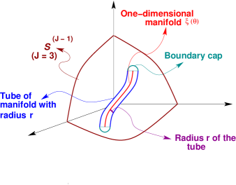
Figure 1: (color) Tube around a one-dimensional manifold ${\mbox{\boldmath$\xi$}}({\mbox{\boldmath$\theta$}})$, with boundaries, embedded in $\mathcal{S}^{2}\subset\mathcal{R}^{3}$.

Except in special cases, this distribution cannot be expressed analytically. However, a good asymptotic solution to the tail probability $P(\sup_{{\mbox{\boldmath$\theta$}}}\,Z({\mbox{\boldmath$\theta$}})\geq c)$, where $c\in\mathcal{R}$ is large, can be obtained via the volume-of-tube formula [7–9]. The volume-of-tube formula provides an elegant geometric approach for solving problems in simultaneous inference [10] by reducing the evaluation of tail probabilities to that of finding the $(J-1)$-dimensional volume of the set of points lying within a distance $r$ of the curve $(d=1)$ or manifold $(d\geq 2)$ on the surface of the unit sphere in $J$-dimensions for some integer $J$ (see Fig. 1).

Suppose ${\mbox{\boldmath$\xi$}}({\mbox{\boldmath$\theta$}})$ defines a manifold for $\theta$ on the surface of a $(J-1)$-dimensional unit sphere $\mathcal{S}^{(J-1)}$. Fig. 1 shows a “tube” of radius $r$ around a manifold ${\mbox{\boldmath$\xi$}}({\mbox{\boldmath$\theta$}})$ embedded in $\mathcal{S}^{(J-1)}\subset\mathcal{R}^{J}$ with boundary caps. We represent the Gaussian random field $Z({\mbox{\boldmath$\theta$}})$, via the Karhunen-Loève expansion [11] as $Z({\mbox{\boldmath$\theta$}})=\sum_{k=1}^{\infty}\vartheta_{k}\;\xi_{k}({\mbox{\boldmath$\theta$}})=\left<{{\mbox{\boldmath$\vartheta$}}},{{\mbox{\boldmath$\xi$}}({\mbox{\boldmath$\theta$}})}\right>$, where $\left<{\cdot},{\cdot}\right>$ denotes the inner product, $\vartheta$ and $\xi$ are vectors and $\vartheta_{k}\sim N(0,1)$. If the Karhunen-Loève expansion is terminated after $J$ terms, then the following relation between the manifold ${\mbox{\boldmath$\xi$}}({\mbox{\boldmath$\theta$}})$ embedded in $\mathcal{S}^{(J-1)}\subset\mathcal{R}^{J}$ and the Gaussian random field $Z({\mbox{\boldmath$\theta$}})$ holds [6]:

$$P\left(\underset{{\mbox{\boldmath$\theta$}}\in\Theta}{\sup}\,Z({\mbox{\boldmath$\theta$}})\geq c\right)$$

$$= \int_{c^{2}}^{\infty}\;P\left(\underset{{\mbox{\boldmath$\theta$}}\in\Theta}{\sup}\,\left<{\mbox{\boldmath$U$}},{{\mbox{\boldmath$\xi$}}({\mbox{\boldmath$\theta$}})}\right>\geq\;w\right)h_{J}(y)\;dy,$$

where $\mbox{\boldmath$U$}=(U_{1}=\vartheta_{1}/\|{\mbox{\boldmath$\vartheta$}}\|,\ldots,U_{J}=\vartheta_{J}/\|{\mbox{\boldmath$\vartheta$}}\|)$ is uniformly distributed on $\mathcal{S}^{(J-1)}\subset\mathcal{R}^{J}$, ${\mbox{\boldmath$\xi$}}=(\xi_{1},\ldots,\xi_{J})$, $w=c/\sqrt{y}$, and $h_{J}(y)$ is a $\chi^{2}$ density with $J$ degrees of freedom. The uniformity property enables finding the $P(\cdot)$ in the integrand via the volume-of-tube formula. Note that $r^{2}=2(1-w)$.

Geometrically, $P(\sup_{{\mbox{\boldmath$\theta$}}}\,\left<{\mbox{\boldmath$U$}},{{\mbox{\boldmath$\xi$}}({\mbox{\boldmath$\theta$}})}\right>\geq\;w)$ is the probability that $U$ lies within a tube of radius $r$ around ${\mbox{\boldmath$\xi$}}({\mbox{\boldmath$\theta$}})$ on the surface of $\mathcal{S}^{(J-1)}$ and equals the volume of tube around ${\mbox{\boldmath$\xi$}}({\mbox{\boldmath$\theta$}})$ divided by the surface area of $\mathcal{S}^{(J-1)}$ [7, 8]. In effect, constructing a test of significance level 5% is equivalent to choosing the rejection set covering 5% of $\mathcal{S}^{(J-1)}$. Therefore, finding critical values of the test statistic ${\mathbb{T}}$ is equivalent to finding a $(J-1)$-dimensional volume of the tube.

The results of Hotelling-Weyl-Naiman [7–9] imply that for $w\approx 1$, the tail probability is expressible as a weighted sum of $\chi^{2}$ distributions, with $(d+1)$ terms and coefficients that depend on the geometry of the $d$-dimensional manifold ${\mbox{\boldmath$\xi$}}({\mbox{\boldmath$\theta$}})$. The results of Pilla and Loader [6] provide an expansion of the distribution of $\sup_{{\mbox{\boldmath$\theta$}}}\,Z({\mbox{\boldmath$\theta$}})$ in terms of the $\chi^{2}$ probabilities:

$$P\left(\sup_{{\mbox{\boldmath$\theta$}}\in\Theta}\,Z({\mbox{\boldmath$\theta$}})\geq c\right)$$ (3)

$$= \;\sum_{k=0}^{d}\frac{\zeta_{k}}{A_{k}A_{d+1-k}}P\left(\chi_{d+1-k}^{2}\geq c^{2}\right)$$

$$+\;o(c^{-1/2}e^{-c^{2}/2})\;\mbox{as}\;c\to\infty,$$

where $A_{0}=1$ and $A_{k}=2\,\pi^{k/2}/\Gamma(k/2)$ for $k\geq 1$. The constants $\zeta_{0},\ldots,\zeta_{d}$ depend on the geometry of the $\xi({\mbox{\boldmath$\theta$}})$; $\zeta_{0}$ is the area of the manifold and $\zeta_{1}$ is the length of the boundary of the manifold. These can be represented explicitly in terms of the covariance function:

$$\zeta_{0}=\int_{{\mbox{\boldmath$\theta$}}\in\Theta}[C({\mbox{\boldmath$\theta$}},{\mbox{\boldmath$\theta$}})]^{-\frac{(d+1)}{2}}\,D({\mbox{\boldmath$\theta$}},{\mbox{\boldmath$\theta$}})\,d{\mbox{\boldmath$\theta$}},$$

where $D({\mbox{\boldmath$\theta$}},{\mbox{\boldmath$\theta$}})$ is defined as

$$\Bigg{|}{\det}\begin{pmatrix}C({\mbox{\boldmath$\theta$}},{\mbox{\boldmath$\theta$}}^{{\dagger}})&\nabla_{1}\,C({\mbox{\boldmath$\theta$}},{\mbox{\boldmath$\theta$}}^{{\dagger}})\\ \nabla_{2}\,C({\mbox{\boldmath$\theta$}},{\mbox{\boldmath$\theta$}}^{{\dagger}})&\nabla_{1}\nabla_{2}\,C({\mbox{\boldmath$\theta$}},{\mbox{\boldmath$\theta$}}^{{\dagger}})\end{pmatrix}\Bigg{|}_{{\mbox{\boldmath$\theta$}}^{{\dagger}}={\mbox{\boldmath$\theta$}}}^{\frac{1}{2}}$$

with $\nabla_{1}$ and $\nabla_{2}$ as the partial derivative operators with respect to $\theta$ and ${\mbox{\boldmath$\theta$}}^{{\dagger}}$ respectively. The expression for $\zeta_{1}$ is similar except that integration is over the boundary of the manifold. The remaining constants involve curvature of the manifold and its boundaries, and become progressively more complex. However, for practical problems the first few terms will suffice and an implementation of the first four terms is described in [12]. When the reference distribution can be approximated by a $\chi^{2}$ distribution, then a tabulated value can be employed to calibrate the test statistic whereas the geometric constants appearing in the above tail probability evaluation depend on the problem at hand. In this modern computer era, it is not difficult to compute them numerically [12].

In many applications, including the one considered in this letter, one is interested in the probabilities of rare events (i.e., $c\rightarrow\infty$). In this case, the terms in Eq. (3) are of descending size, and the error term is asymptotically negligible.

Figure 2: (color) Surface of the process ${\rm S}^{\star}({\mbox{\boldmath$\theta$}})$ as a function of ${\mbox{\boldmath$\theta$}}=(E_{0},\Gamma)$.

We demonstrate the power of the score test with a Monte Carlo simulation experiment drawn from high-energy physics. In our simulation, we consider measurements of energy in a region $E\in[0,2]$ in which the background (null) density is modeled as linear, with a specific form $f(E)=(1/2.6)\,(1+0.3E)$. The resonance is modeled by a Breit-Wigner density function. The parameters for this problem are modeled following an example in Roe [13].

To examine the effectiveness of the test ${\mathbb{T}}$ in detecting a signal, we perform Monte Carlo analyses of 10,000 samples each with a size of $n=1000$ events spread over 50 bins at the values of $\Gamma=0.2$ and $E_{0}=1$. For a single simulated dataset, Fig. 2 shows the normalized score surface as a function of $E_{0}$ and $\Gamma$. It is clear that the maximum is achieved at $E_{0}=1$ irrespective of the value of $\Gamma$.

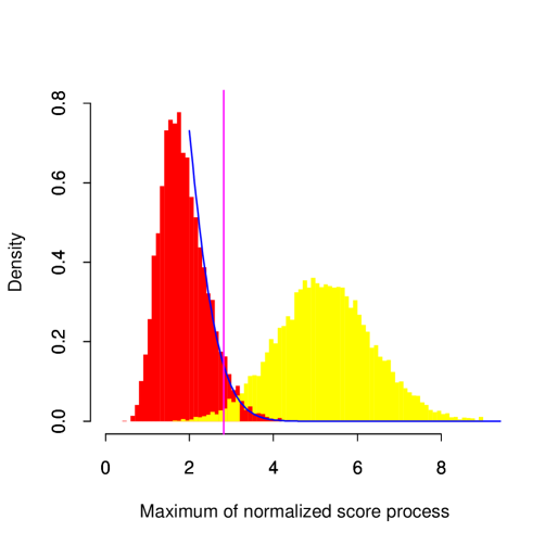
Figure 3: (color) Histograms of the simulated null ($\eta=0$) density (red) and alternative ($\eta=0.1$) density (yellow) of the test statistic ${\mathbb{T}}$ with a superimposed (blue) asymptotic null density (derivative of Eq. [3]) for a fixed $\Gamma$. The purple vertical bar is the cut off for the test statistic ${\mathbb{T}}$ at the 5% false positive rate calculated via the volume-of-tube formula (Eq. [3] with $d=1$).

Fig. 3 shows histograms over 10,000 samples under the $\mathcal{H}_{0}\!:\eta=0$ and $\mathcal{H}_{1}\!:\eta=0.1$ for a fixed $\Gamma$. The former histogram confirms that about 5% of the time, hypothesis of no signal be rejected. The asymptotic null density (derivative of Eq. [3] with $d=1$) agrees with the simulated null distribution as expected.

When both $E_{0}$ and $\Gamma$ are estimated, Fig. 4 shows that the power of detection increases as the signal strength $\eta$ increases. Our test statistic ${\mathbb{T}}$ is significantly more powerful than the $\chi^{2}$ goodness-of-fit test in detecting the signal. The asymptotic tail probability result obtained via the volume-of-tube formula (Eq. [3]) is elegant, simple and powerful in distinguishing the signal and the random fluctuations in data.

Financial support from the U.S. National Science Foundation, Division of Mathematical Sciences and the Office of Naval Research, Probability & Statistics Program is gratefully acknowledged.

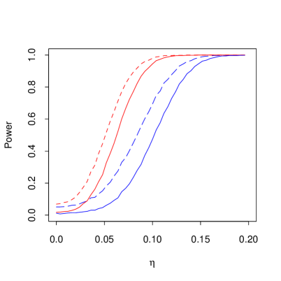
Figure 4: (color) Power comparison of the $\chi^{2}$ goodness-of-fit test (blue) and normalized score test ${\mathbb{T}}$ (red) for $d=2$ at $\alpha=0.05$ (dashed) and $\alpha=0.01$ (solid), calculated via the volume-of-tube formula, based on 10,000 simulations for binned data.

1. Wilks, S.S. Mathematical Statistics. (Princeton University Press, New Jersey, 1944).

2. Eadie W.T. et al.. Statistical Methods in Experimental Physics (New York: North-Holland, 1971).

3. Cranmer, K.S. PHYSTAT2003, SLAC, Stanford, California (2003).

4. Freeman, P.E. et al. Astrophys. J. 524, 1, 753 (1999).

5. Protassov, R. et al. Astrophys. J. 571, 1, 545 (2002).

6. Pilla, R.S. & Loader, C. Technical Report, Department of Statistics, Case Western Reserve University (2003).

7. Hotelling, H. Amer. J. Math. 61, 440 (1939).

8. Weyl, H. Amer. J. Math. 61, 461 (1939).

9. Naiman, D.Q. Ann. Stat. 18, 685 (1990).

10. Knowles, M. & Siegmund, D. Intl. Stat. Rev. 57, 205 (1989).

11. Adler, R.J. An introduction to Continuity, Extrema and Related Topics for General Gaussian Processes. (Institute of Mathematical Statistics, Hayward, CA, 1990).

12. Loader, C. Computing Science and Statistics: Proc. 36th Symp. Interface (2004).

13. Roe, B.P. Probability and Statistics in Experimental Physics. (Springer, NY, 1992).