Multiple Projection Optical Diffusion Tomography with Plane Wave Illumination

Abstract

We describe a new data collection scheme for optical diffusion tomography in which plane wave illumination is combined with multiple projections in the slab imaging geometry. Multiple projection measurements are performed by rotating the slab around the sample. The advantage of the proposed method is that the measured data can be much more easily fitted into the dynamic range of most commonly used detectors. At the same time, multiple projections improve image quality by mutually interchanging the depth and transverse directions, and the scanned (detection) and integrated (illumination) surfaces. Inversion methods are derived for image reconstructions with extremely large data sets. Numerical simulations are performed for fixed and rotated slabs.

1 Introduction

Tomographic imaging with diffuse light, often referred to as optical diffusion tomography (ODT), is a novel biomedical imaging modality [1, 2]. Although ODT was introduced more than a decade ago, efforts to bring it into the clinical environment are hampered by relatively low quality and spatial resolution of images. Therefore, optimization of image reconstruction algorithms for high-resolution ODT is of fundamental importance. In this paper we study the image reconstruction problem of ODT by combining three novel approaches. First, we employ analytic image reconstruction methods which allows the utilization of extremely large data sets [3, 4]. Second, we make use of multiple projections [5]. Here by multiple projections we mean multiple orientations of the measurement apparatus with respect to the medium. Finally, we utilize the recently proposed plane wave illumination scheme [6]. Each of these methods provides an advantage which is not lost when the techniques are combined. We begin by briefly reviewing the approaches to ODT imaging mentioned above. Note that throughout this paper we consider the slab imaging geometry which is often used in mammography and small-animal imaging [7, 8]. In order to obtain multiple projection measurements, a pair of parallel plates are rotated around the medium to be imaged which is assumed to be stationary and unperturbed.

There is a direct relationship between the spatial resolution of images and the number of data points used for reconstruction [3]. Indeed, the reconstruction of an image with $N$ voxels, in principle, requires at least $N$ measurements. In practice, the ill-posedness of the image reconstruction problem and the presence of noise require that this number be larger than $N$. Measurements with up to $10^{10}$ data points are feasible with CCD camera-based instruments. However, many previous studies of the image reconstruction problem in ODT have been limited to relatively small data sets (e.g., 256 data points in Ref. [9], 900 data points in Ref. [10]). This can be explained by the high computational complexity of algebraic image reconstruction algorithms which scales as $O(N^{3})$. To ameliorate this difficulty, we have recently introduced a family of analytic image reconstruction algorithms that can utilize extremely large data sets [11, 12, 13, 14, 15]. These methods allow a dramatic reduction in computational complexity which, in turn, leads to a significant improvement of spatial resolution of images. However, these methods have certain limitations.

First, the data collection method described in Ref. [14] requires that measurements are taken for source-detector pairs separated by a distance which is much larger than the slab thickness. In practice, such measurements are technically difficult to perform. Reduction of the required dynamic range of the detectors can be achieved by using plane wave illumination [6]. Note that due to the general theoretical reciprocity of sources and detectors, plane wave illumination and scanned detection is equivalent to integrated detection and scanned narrow beam illumination. However, in a practical situation, the different nature of illuminating and detecting devices must be taken into account. For the sake of definitiveness, we consider below plane wave illumination and combine it with analytic image reconstruction methods. Note that plane wave illumination requires time- or frequency-resolved measurements. However, it can be seen that the number of degrees of freedom in the data is still insufficient for unique, simultaneous reconstruction of the absorption and diffusion (or reduced scattering) coefficients. This situation is similar to the nonuniqueness demonstrated in Ref. [16]. Therefore, we focus here on the reconstruction of absorbing inhomogeneities assuming that the diffusion coefficient of the medium is constant. Reconstruction of purely absorbing inhomogeneities have been employed, for example, in breast imaging [17, 18, 19, 20] or blood oxygenation level imaging [21, 22].

Second, it was shown in Ref. [3] that in the slab imaging geometry the depth resolution (in the direction perpendicular to the slab) is fundamentally different from the transverse resolution (in the direction parallel to the slab surface). The depth resolution is much more sensitive to noise and the point-spread functions (PSFs) in the depth direction strongly depend on the location of the inhomogeneity. This results in image artifacts. In general, the non-uniformity of the PSF can be a serious problem if more than one inhomogeneity is present. To correct this situation, we have recently proposed multi-projection image reconstruction methods [5, 15]. Multiple projections render the depth and transverse directions mutually interchangeable. As a result, the PSF becomes more uniform and less position-dependent, and also more sharply peaked. Note that multiple projections have been used in X-ray imaging for some time. However, an important difference between ODT and X-ray computed tomography is that, in the first case, tomographic imaging is possible in principle with a single projection while in the second case it is not. Perhaps, due to this fact, multiple projections in optical tomography have not been investigated until recently, except for the case of ballistic propagation without scattering (e.g. [23]), or in conjunction with a modified version of X-ray backprojection tomography with phenomenological corrections introduced to compensate for scattering [24, 25]. In Ref. [15] we have developed a general theoretical formalism for inverting measurements obtained from multiple projections. In Ref. [5] image reconstruction with two orthogonal projections was numerically implemented.

In this paper we implement the more general image reconstruction algorithm of Ref. [15] for treatment of more than two projections in conjunction with plane wave illumination. Note that the plane wave illumination is advantageous when measurement are limited by the dynamic range of detectors. If the dynamic range is not an important experimental factor, the traditional measurement scheme with point sources and point detectors is expected to provide superior image quality. We combine the advantageous features of these two approaches with the computational efficiency of the analytic image reconstruction methods.

2 Theory

2.1 Single projection

We assume that propagation of multiply-scattered light in tissue is described by the diffusion equation. In addition, we will work in the frequency domain with the sources harmonically modulated at the frequency $\omega$ and detectors which yield the oscillatory part of transmitted intensity. Then the density of electromagnetic energy in the medium $u({\bm{r}})$ obeys the diffusion equation

$$-D_{0}{\bm{\nabla}}^{2}u({\bf r})+[\alpha({\bf r})-i\omega]u({\bf r})=S({\bf r})\ ,$$ (1)

where $\alpha({\bm{r}})$ is the position dependent absorption coefficients, $S({\bm{r}})$ is the source function and the $D_{0}$ is the diffusion coefficient.

Consider a slab of thickness $L$ with the plane of incidence located at $x=-L/2$ and the detection plane at $x=L/2$. The medium is located in the region $-L/2<x<L/2$. If point-like sources and detectors are used (typically, thin optical fibers), the data can be expressed as a function $\phi(\omega,{\bm{\rho}}_{s},{\bm{\rho}}_{d})$, where ${\bm{\rho}}_{s}$ and ${\bm{\rho}}_{d}$ are two-dimensional vectors specifying the location of the sources and detectors, respectively, on the slab surfaces. Using the first Born approximation, we linearize the forward model by decomposing the absorption function $\alpha({\bm{r}})$ into a constant background and a small fluctuating part, $\alpha({\bm{r}})=\alpha_{0}+\delta\alpha({\bm{r}})$. We seek to reconstruct the values of $\delta\alpha({\bm{r}})$ from the data $\phi(\omega,{\bm{\rho}}_{s},{\bm{\rho}}_{d})$. The usual mathematical formulation of the ODT inverse problem is based on the integral equation [26]

$$\phi(\omega,{\bm{\rho}}_{s},{\bm{\rho}}_{d})=\int\Gamma(\omega,{\bm{\rho}}_{s},{\bm{\rho}}_{d};{\bm{r}})\delta\alpha({\bm{r}})d^{3}r\ ,$$ (2)

where

$$\Gamma(\omega,{\bm{\rho}}_{s},{\bm{\rho}}_{d};{\bm{r}})= \int{{d^{2}q_{s}d^{2}q_{d}}\over{(2\pi)^{4}}}\kappa(\omega,{\bm{q}}_{s},{\bm{q}}_{d};x)$$ (3)

$$\times\exp\left[i{\bm{q}}_{s}\cdot\left({\bm{\rho}}-{\bm{\rho}}_{s}\right)+i{\bm{q}}_{d}\cdot\left({\bm{\rho}}_{d}-{\bm{\rho}}\right)\right]\ ,$$

${\bm{\rho}}$ is the transverse part of the vector ${\bm{r}}$ (${\bm{r}}=(x,{\bm{\rho}})$) and the form of $\kappa(\omega,{\bm{q}}_{s},{\bm{q}}_{d};x)$ is determined from the boundary conditions on the surfaces of the slab and the expression which relates the measurable intensity to the energy density $u({\bm{r}})$. The derivation of (2),(3) and explicit expressions for $\kappa$ are given in Ref. [3]. Note that the general form of (2),(3) follows from the symmetry of the problem and is independent of the diffusion approximation.

Next, we introduce the plane wave illumination scheme. Instead of using point sources located at points ${\bm{\rho}}_{s}$, we illuminate the slab with a normally incident wide homogeneous beam of sufficiently large diameter (compared to transverse dimensions of the slab). At the same time we utilize point detectors. This ensures that the new data function $\psi(\omega,{\bm{\rho}}_{d})$ defined by

$$\psi(\omega,{\bm{\rho}}_{d})=\int\phi(\omega,{\bm{\rho}}_{s},{\bm{\rho}}_{d})d^{2}\rho_{s}$$ (4)

has the same number of degrees of freedom as the unknown $\delta\alpha({\bm{r}})$ (two spatial directions and the frequency $\omega$). Thus, the inverse problem is well determined. The integral equation (2) can now be transformed to

$$\psi(\omega,{\bm{\rho}}_{d})=\int{{d^{2}q}\over{(2\pi)^{2}}}\kappa(\omega,0,{\bm{q}};x)\exp[i{\bm{q}}\cdot({\bm{\rho}}_{d}-{\bm{\rho}})]\delta\alpha({\bm{r}})d^{3}r\ .$$ (5)

If $\psi$ is measured for $N$ different modulation frequencies and the sources are placed on a square lattice with step size $h$, Eq. (5) can be inverted using the methods described in [14]. The SVD pseudo-inverse solution is given by

$$\delta\alpha({\bm{r}})=h^{2}\int_{\rm FBZ}{{d^{2}u}\over{(2\pi)^{2}}}\exp(-i{\bm{u}}\cdot{\bm{\rho}})\sum_{\omega,\omega^{\prime}}P^{*}(\omega,{\bm{u}};{\bm{r}})\langle\omega|M^{-1}({\bm{u}})|\omega^{\prime}\rangle\tilde{\psi}(\omega^{\prime},{\bm{u}})\ .$$ (6)

Here the vector ${\bm{u}}$ is in the first Brillouin zone (FBZ) of the lattice of sources, namely, $-\pi/h<u_{y,z}\leq\pi/h$ and

$$P(\omega,{\bm{u}};{\bm{r}})=\sum_{\bm{v}}\kappa(\omega,0,{\bm{u}}+{\bm{v}};x)\exp(i{\bm{v}}\cdot{\bm{\rho}})\ ,$$ (7)

where ${\bm{v}}$ are reciprocal lattice vectors of the form ${\bm{v}}=(2\pi/h)(n_{y}\hat{\bm{y}}+n_{z}\hat{\bm{z}})$. The elements of matrix the $M({\bm{u}})$ are given by

$$\langle\omega|M({\bm{u}})|\omega^{\prime}\rangle=\sum_{\bm{v}}M_{1}({\bm{u}}+{\bm{v}})\ ,$$ (8)

where

$$\langle\omega|M_{1}({\bm{q}})|\omega^{\prime}\rangle=\int_{-L/2}^{L/2}\kappa(\omega,0,{\bm{q}};x)\kappa^{*}(\omega^{\prime},0,{\bm{q}};x)dx$$ (9)

(the inverse matrix $M^{-1}({\bm{u}})$ must be appropriately regularized [27]) and the Fourier transformed data function $\tilde{\psi}(\omega,{\bm{u}})$ is defined as

$$\tilde{\psi}(\omega,{\bm{u}})=\sum_{{\bm{\rho}}_{d}}\psi(\omega,{\bm{\rho}}_{d})\exp(i{\bm{u}}\cdot{\bm{\rho}}_{d})\ .$$ (10)

Note that, if $\delta\alpha$ is reconstructed only at points which are commensurate with the lattice of sources, the factor $\exp(i{\bm{v}}\cdot{\bm{\rho}})$ is equal to unity and the function $P$ becomes independent of ${\bm{\rho}}$. Note also that $\kappa$ and $M_{1}$ can be calculated in terms of elementary functions [15].

2.2 Multiple projections

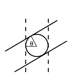
Figure 1: A sketch of the experimental set up with rotating slab. The axis of rotations ($Oz$) is perpendicular to the plane of the figure and coincides with the axis of the cylinder $R<L/2$ inside which reconstructions are performed. Locations of sources and detectors are given in a local reference frame which rotates together with the slab.

We now consider inclusion of multiple projections. Let the sources and detectors be rotated around the sample as illustrated in Fig. 1. We assume that the rotations do not disturb the medium inside the cylinder $\sqrt{x^{2}+y^{2}}<L/2$ and that the unknown function $\delta\alpha$ vanishes outside the same region. The space inside the slab but outside the above cylindrical region is assumed to have the background values of the coefficients $\alpha_{0}$ and $D_{0}$. Experimentally, this can be implemented, for example, by rotating an imaging apparatus around a sample suspended in matching fluid. We introduce cylindrical coordinates ${\bm{r}}=(R,z,\varphi)$ with the $z$-axis being the axis of rotation. If the data are measured for $N_{\theta}$ different orientations, where the respective angles $\theta_{n}$ are equally spaced and given by $\theta_{n}=2\pi(n-1)/N_{\theta},\ n=1,\ldots,N_{\theta}$, the reconstruction formula (6) can be generalized to [15]:

$$\delta\alpha({\bm{r}})={{2\pi h^{2}}\over{N_{\theta}}}\sum_{n=1}^{N_{\theta}}\int_{-\pi/h}^{\pi/h}{{du_{z}}\over{2\pi}}\exp[-i(u_{z}z+n\varphi)]\sum_{\omega,\omega^{\prime}}\int_{-\pi/h}^{\pi/h}du_{y}\int_{-\pi/h}^{\pi/h}du_{y}^{\prime}P^{*}(\omega,{\bm{u}},n;{\bm{r}})$$

$$\times\langle\omega,u_{y}|M^{-1}(u_{z},n)|\omega^{\prime},u_{y}^{\prime}\rangle\tilde{\psi}(\omega^{\prime},u_{y}^{\prime},u_{z},n)\ .$$ (11)

Here

$$P(\omega,{\bm{u}},n;{\bm{r}})=\sum_{k=-\infty}^{\infty}\sum_{\bm{v}}a(\omega,{\bm{u}}+{\bm{v}},n+N_{\theta}k;R)\exp[i(N_{\theta}k\varphi+v_{z}z)]\ ,$$ (12)

$$a(\omega,{\bm{q}},m;R)=\int_{0}^{2\pi}\kappa(\omega,0,{\bm{q}};R\cos\varphi)\exp[i(q_{y}R\sin\varphi-m\varphi)]d\varphi\ ,$$ (13)

the elements of the matrix $M(u_{z},n)$ are given by

$$\langle\omega,u_{y}|M(u_{z},n)|\omega^{\prime},u_{y}^{\prime}\rangle=\sum_{k=-\infty}^{\infty}\sum_{v_{y},v_{y}^{\prime}}\sum_{v_{z}}\langle\omega,u_{y}+v_{y}|M_{1}(u_{z}+v_{z},n+N_{\theta}k)|\omega^{\prime},u_{y}^{\prime}+v_{y}^{\prime}\rangle\ ,$$

(14)

$$\langle\omega,q_{y}|M_{1}(q_{z},m)|\omega^{\prime},q_{y}^{\prime}\rangle=\int_{0}^{L/2}a(\omega,q_{y},q_{z},m;R)a^{*}(\omega^{\prime},q_{y}^{\prime},q_{z},m;R)RdR$$ (15)

and the Fourier-transformed data function is

$$\tilde{\psi}(\omega,{\bm{u}},n)=\sum_{{\bm{\rho}}_{d},\theta}\psi(\omega,{\bm{\rho}}_{d},\theta)\exp[i({\bm{u}}\cdot{\bm{\rho}}_{d}+n\theta)]\ .$$ (16)

Note that in (16) we have explicitly included the dependence of the data function on the angle of orientation $\theta$. The functions $a(\omega,{\bm{q}},m;R)$ and $\langle\omega,q_{y}|M_{1}(q_{z},m)|\omega^{\prime},q_{y}^{\prime}\rangle$ can be, in general, expressed in terms of modified Bessel functions. The corresponding integrals (13) and (15) are calculated in the Appendix for the case of purely absorbing boundaries.

A few comments on the reconstruction formula (11) are necessary. First, there is an apparent difference between the variables $u_{z},n$ and $u_{y},\omega$. The first set of variables correspond (after Fourier transformation of the data) to the variables $z,\theta$. These are the variables with respect to which the unperturbed medium is translationally invariant, and they can be referred to as “external” variables. The variables $\omega,u_{y}$ are “internal” variables: they do not correspond to any translational invariance of the system. Second, the reconstruction algorithm (16) involves integration over the continuous variables $u_{y}$ and $u_{y}^{\prime}$ and inversion of the operator $M(u_{z},n)$ whose matrix elements depend on continuous indices. However, if the variables $u_{y},u_{y}^{\prime}$ are discretized and the corresponding integration in (16) is replaced by a summation, then $M(u_{z},n)$ becomes a discrete matrix. The resulting reconstruction formula is no longer an SVD pseudo-inverse on the whole set of data $\psi(\omega,{\bm{\rho}}_{d},\theta)$. However, it is a pseudo-inverse solution on the set of the Fourier-transformed data $\tilde{\psi}(\omega,u_{y},u_{z},\theta)$ where $u_{y}$ takes only discrete values. Third, it can be verified that in the case $N_{\theta}=1$, the reconstruction formula (16) reduces to (6). Fourth, we note that the number of degrees of freedom in the data-function $\tilde{\psi}$ is four ($\omega,u_{y},u_{z}$ and $n$). Thus, when the number of rotations is large, it is sufficient to use only one or a few values of the variable $u_{y}$, in which case the inverse problem is still well determined. It can be argued that the reconstruction algorithm is then “numerical” in one dimension and “analytic” in two.  However, when only a small number of projections is taken, we must use a relatively large number of discrete values of $u_{y}$. By doing so, we increase the size of the matrix $M$ whose SVD must be found numerically. The inverse solution (11) is then “numerical” in two dimensions and “analytic” in one. A similar algorithm (numerical in two dimensions and analytic in one dimension) was proposed and implemented in [5], where the image reconstruction area was rectangular rather than cylindrical, but only two orthogonal projections were allowed. In contrast, the full potential of the image reconstruction algorithm proposed here is realized when $N_{\theta}$ is large.

3 Numerical Results

3.1 Single projection

We have implemented the proposed reconstruction algorithm using computer-generated data and the following parameters: the slab thickness was chosen to be the same as the cw diffuse wavelength, $L=2\pi\sqrt{D_{0}/\alpha_{0}}$ (for most biological tissues, this corresponds to $L\sim 6{\rm cm}$); the lattice step was chosen to be $h=L/40$ and we have used $N=25$ different modulation frequencies which range from $\omega=0$ to $\omega=10\alpha_{0}$ (the maximum frequency corresponds to $\sim 1.6{\rm GHz}$); the field of view was chosen to be $L\times L$ and, finally, we have generated forward data for a single point (delta-function) absorber which is located in the center of the field of view but at different depths. Absorbing boundary conditions were imposed on the surface of the slab. The corresponding expression for the function $\kappa(\omega,0,{\bm{q}};x)$ is given in the Appendix.

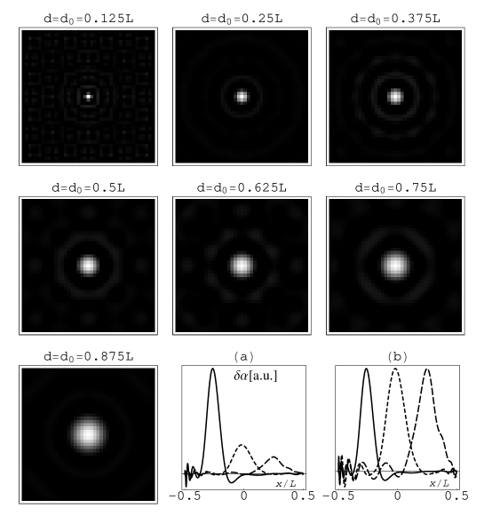
Figure 2: Tomographic slices parallel to the slab surface drawn through the medium at different depths $d$ (from the plane of scanned detection) with the small absorber lying in the center of the field of view at the same depth $d_{0}=d$, and the point-spread functions representing depth resolution (a,b). The curves are plotted on the same scale (a) and normalized to their own maxima (b). For curves (a,b), the point absorber depth is $d_{0}=0.25L$ (solid line), $d_{0}=0.5L$ (short dash) and $d_{0}=0.75L$ (long dash).

The results of reconstructions are shown in Fig. 2. The density plots represent tomographic slices of the medium drawn at different depths $d$ (the distance from the plane of scanned detection) parallel to the slab surfaces. The depth of the absorbing inhomogeneity, $d_{0}$, was in each case equal to $d$; thus the slices represent the depth-dependent $y-z$ PSFs. Each density plot has a linear color scale and is normalized to its own maximum. As expected, the PSFs become broader when the point absorber approaches the illuminated plane. The last two panels (a,b) show the PSFs in the depth direction ($x$) for point absorbers located at $d_{0}=0.25L$, $d_{0}=0.5L$ and $d_{0}=0.75L$. Note that the approximate half-widths of these curves are $0.06L$, $0.09L$ and $0.09L$, respectively.

The analysis of Fig. 2 suggests that the PSFs are depth-dependent. Moreover, the PSFs have different integral weights. Thus, the point absorbers which are closer to the plane of scanned detection result in higher peaks in the reconstructed images. The width of the PSFs also depends on depth of the point absorber. This potentially constitutes a serious problem for three dimensional tomographic imaging.

3.2 Multiple projections

We have implemented numerically the multi-projection image reconstruction formula (11). Note that in the multi-projection case there are two choices for graphically representing the tomographic slices. In one case, the slices are perpendicular to the axis of rotation. The image then is reconstructed in a circle. This choice is convenient for studying the radial and angular resolutions. Another possibility is to construct cylindrical slices $R=R_{\rm image}={\rm const}$, and map them onto rectangles. The image is then reconstructed in the rectangular area $2\pi R_{\rm image}\times(z_{\rm max}-z_{\rm min})$, where $z_{\rm max}$ and $z_{\rm min}$ are the maximum and minimum values of $z$, chosen arbitrarily.

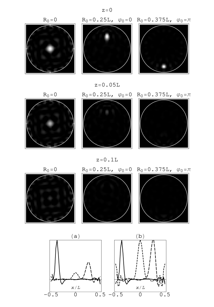
Figure 3: Circular slices illustrating radial, angular and $z$ resolution. All point absorbers are in the $z=0$ plane, and the point-spread functions representing depth ($R$) resolution (a,b). The radial and angular coordinates of the point absorber, $R_{0}$ and $\varphi_{0}$, are specified in the figure legends. First row of images: slices at $z=0$; second row: slices at $z=0.05L$; third row: slices at $z=0.1L$. Images (a-b): reconstruction along the diameter that crosses all three inhomogeneities. In (a,b) solid line corresponds to $R_{0}=0.375L$ and $\varphi_{0}=\pi$, short dash to $R_{0}=0$ and long dash to $R_{0}=0.25L$ and $\varphi_{0}=0$ Four projections, $15$ modulation frequencies and $23$ discrete values of $u_{y}$ are used.

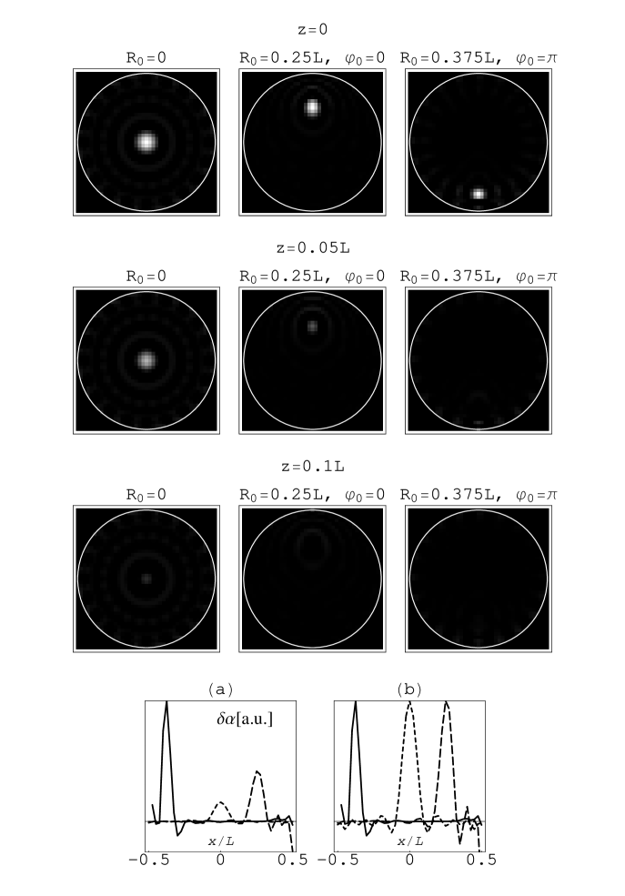
Figure 4: Same as in Fig. 3 but $20$ projections are used.

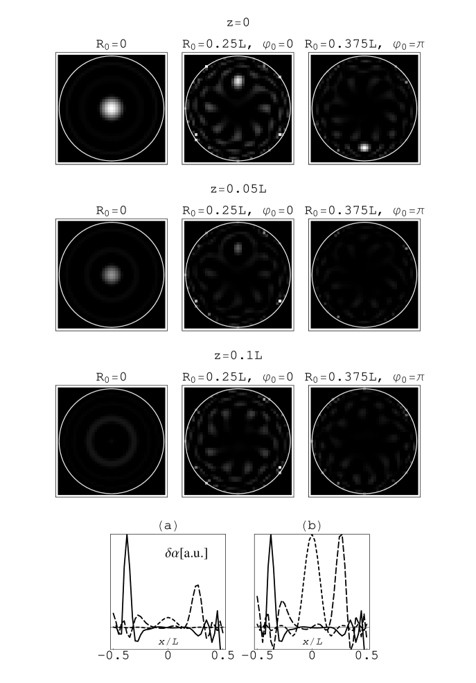
Figure 5: Same as in Fig. 3 but $40$ projections and only three discrete values of $u_{y}$ are used.

We start with the discussion of circular slices. The results of numerical implementation of the reconstruction formula (16) are shown in Fig. 3 for four different orientations of the slab, namely $\theta=0,\pi/2,\pi,3\pi/2$. We have used $23$ equally spaced values of $u_{y}$ ranging from $-\pi/h$ to $\pi/h$ and $15$ equally spaced modulation frequencies ranging from $0$ to $10\alpha_{0}$; otherwise, the parameters are the same as in Fig. 2. The inhomogeneity was located as specified in the figure legend. The white spots in the density plots illustrate the depth PSFs. The graphs (a,b) show the same PSFs in a more quantitative way by plotting $\delta\alpha$ along the diameter of the cylinder which intersects all three inhomogeneities.

As expected, using four different projections improves the image quality by interchanging the source and detector planes, and the depth and transverse directions. Moreover, using more projections than four does not change the results substantially, as is illustrated in Figs. 4 and 5. However, when a large number of projections is taken, the inverse problem becomes well determined even when a relatively small number of “internal” degrees of freedom $u_{y}$ is used. This makes the reconstruction formulae computationally efficient. Thus, the computation time required for producing data for Fig. 5 is more than an order of magnitude less than that for Fig. 3, yet the image quality is similar. We have verified that three discrete values of $u_{y}$ is also sufficient for $N_{\theta}=20$ (taking a single value $u_{y}=0$ results in a slight decrease in image quality; data not shown).

Although the images shown in Figs. 3-5 are similar, the best image quality is, in fact, attained in Fig. 4. Here the approximate half-widths of the PSF in the $R$ direction are $0.05L$ for the inhomogeneity located at $R_{0}=0$, $0.04L$ for the inhomogeneity at $R_{0}=0.25L$, $\varphi_{0}=0$; and $0.03L$ for the inhomogeneity at $R_{0}=0.375L$, $\varphi_{0}=\pi$. These values should be compared to the respective values given in the discussion of Fig. 2. In particular, the inhomogeneity located at $h_{0}=0.5L$ in Fig. 2 corresponds to the inhomogeneity at $R_{0}=0$ in Figs. 3-5 and is the most “difficult” to reconstruct since it is located deep inside the medium. It can be seen that the PSF half-width in the image of this particular inhomogeneity is reduced by approximately the factor of $2$ due to the use of multiple projections. In addition, the relative heights of the maxima of the PSFs in Fig. 3-5 do not differ as much as in Fig. 2. This is expected to reduce image artifacts.

Now we consider the cylindrical slices. From the computational point of view, the use of cylindrical slices is a more natural way to display reconstructed images. This is evident from the inversion formulae (11),(12). Indeed, it can be seen that when the reconstructed image is rasterized so that the variables $z$ and $\varphi$ are placed on lattices with steps $h$ and $2\pi/N_{\theta}$, respectively, the function $P(\omega,{\bm{u}},n;R,z,\varphi)$ becomes independent of $z$ and $\varphi$. Then the dependence of reconstructed images on these two variables is only due to the exponent in the integral (11) and the reconstruction formula, with respect to these two variables, is reduced to a Fourier transform. In Fig. 6 we have used three discrete values of $u_{y}$ with $40$ different projections and slices are drawn as described in the figure caption. Fig. 6(a) illustrates image reconstruction with noiseless data. It can be directly compared to slices shown in Fig. 2. To demonstrate the stability of image reconstruction, we have added random Gaussian noise to the data function at the level of 1% of the average absolute value of the data. The result is shown in Fig. 6(b). As is well known, inclusion of noise tends to decrease spatial resolution. It can be seen that this effect is stronger for inhomogeneities that are deeper inside the medium. We have demonstrated earlier that multi-projection imaging is more stable in the presence of noise than the single projection technique [5].

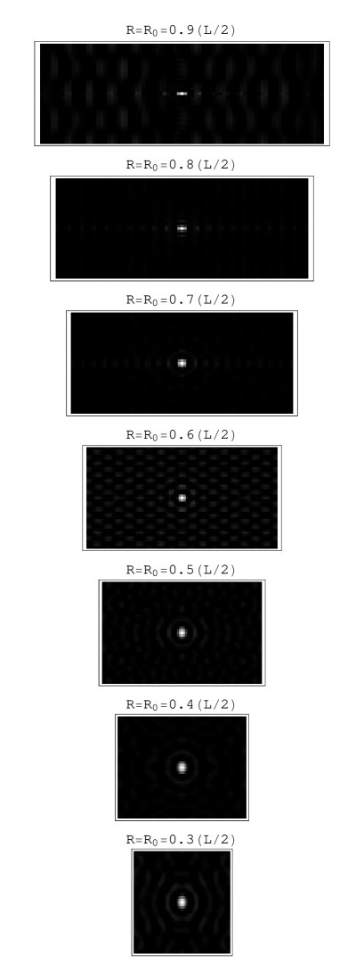
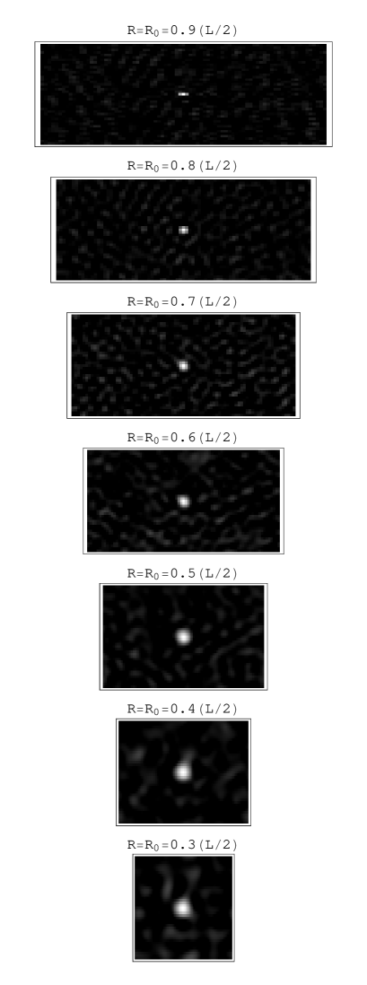
(a)                                                              (b)

Figure 6: Cylindrical slices illustrating $z$ and $\varphi$-resolution for zero noise level (a) and for $1\%$ noise-to-signal ratio (b). The point absorbers are located in the $z=0$ plane at radial depths $R_{0}$ as indicated. The cylindrical surfaces with radii $R=R_{0}$ (directly intersecting the inhomogeneity) are shown as projections onto a plane; the length of the vertical side of each rectangle is equal to $L$ and of the horizontal side to $2\pi R$. Forty projections, $25$ modulation frequencies and $9$ discrete values of $u_{y}$ are used for reconstruction.

4 Summary

In summary, we have presented a new experimental modality and computationally efficient image reconstruction algorithms for optical diffusion tomography employing plane wave illumination with multiple projections. Note that due to reciprocity, plane wave illumination and scanned detection is equivalent to illumination by a scanned narrow beam and integrated detection (e.g., with the use of time-resolved CCD camera). The following specific conclusions can be drawn

• Use of plane wave illumination may be simpler experimentally than the traditional approach in which point-like sources and detectors are scanned because measurements with a much smaller dynamic range are required.

• In a single projection experiment, the image quality is relatively good when the point absorber is close to the scanned surface and deteriorates as it approaches the plane of illumination. This situation should be contrasted with the traditional point source/point detector modality [14], where the image quality is low for inhomogeneities located in the center of a slab and improves when the inhomogeneity approaches either of the imaging surfaces. For a point inhomogeneity in the center of a slab, the image quality is slightly better for the traditional (point source/point detector) modality (cf. [14]).

• Rotating the slab around the sample removes many of the deficiencies of the plane wave illumination scheme by interchanging the scanned and integrated detection surfaces and depth and transverse directions. A minimum of four projections is required for such an interchange.

• When only four rotations are used, a large number of discrete values of the “internal” variable $u_{y}$ must be utilized in the reconstruction. Alternatively, a large number of projections can be used with a small number of discrete values of $u_{y}$. The second approach is much more computationally efficient but requires more complicated measurements. The quality of images is similar in both cases.

• The plane wave illumination approach allows one to significantly simplify reconstruction formulae, both in single- and multiple-projection imaging.

• If only small number of projections is used (two or four) an alternative approach may be used, which is purely numerical in two dimensions and analytic in one dimension [5]. For a large number of projections, the algorithm reported here is computationally more efficient.

This work was supported in part by the AFOSR under the grant F41624-02-1-7001 and by the NIH under grant P41RR0205.

Appendix: Calculation of the functions $a(\omega,{\bm{q}},m;R)$ and $M_{1}(q_{z},m)$.

The function $a(\omega,{\bm{q}},m;R)$ is defined by (13). To evaluate the integral, we must specify the function $\kappa(\omega,0,{\bm{q}};x)$. Explicit expressions for $\kappa$ are given in [3] for general boundary conditions. In this paper we consider absorbing boundaries for which $\kappa$ is given by the expression

$$\kappa(\omega,0,{\bm{q}};x)=\left({\ell^{*}\over D_{0}}\right)^{2}{{\sinh[k(L/2-x)]\sinh[Q(L/2+x)]}\over{\sinh(kL)\sinh(QL)}}\ ,$$ (A1)

where $\ell^{*}=3D_{0}/c$ is the transport mean free path, $c$ is the average speed of light in the medium, $k=\sqrt{(\alpha_{0}-i\omega)/D_{0}}$ is the complex diffuse wavenumber, $Q=\sqrt{q^{2}+k^{2}}$ and ${\bm{q}}=(q_{y},q_{z})$. Generalization to mixed boundaries of Robin type is straightforward and is not discussed here. Then, the expression for $a(\omega,{\bm{q}},m;R)$ becomes

$$a(\omega,{\bm{q}},m;R)=\left({\ell^{*}\over D_{0}}\right)^{2}{1\over{\sinh(kL)\sinh(QL)}}$$

$$\times\int_{0}^{2\pi}\sinh[k(L/2-R\cos\varphi)]\sinh[Q(L/2+R\cos\varphi)]\exp[i(q_{y}R\sin\varphi-m\varphi)]d\varphi\ .$$

This can be equivalently rewritten as

$$a(\omega,{\bm{q}},m;R)=\left({\ell^{*}\over D_{0}}\right)^{2}{1\over{4\sinh(kL)\sinh(QL)}}$$

$$\times\biggl{\{}\exp\Bigl{[}(Q+k)L/2\Bigr{]}F_{m}\Bigl{[}(Q-k)R,iq_{y}R\Bigr{]}-\exp\Bigl{[}(-Q+k)L/2\Bigr{]}F_{m}\Bigl{[}(-Q-k)R,iq_{y}R\Bigr{]}\biggr{.}$$

$$-\biggl{.}\exp\Bigl{[}(Q-k)L/2\Bigr{]}F_{m}\Bigl{[}(Q+k)R,iq_{y}R\Bigr{]}+\exp\Bigl{[}(-Q-k)L/2\Bigr{]}F_{m}\Bigl{[}(-Q+k)R,iq_{y}R\Bigr{]}\biggr{\}}$$

where

$$F_{m}(u,v)=\int_{0}^{2\pi}\exp[u\cos\varphi+v\sin\varphi-im\varphi]d\varphi=2\pi\left({\sqrt{u^{2}+v^{2}}\over{u+iv}}\right)^{m}I_{m}(\sqrt{u^{2}+v^{2}})\ ,$$

and $I_{m}(x)$ is the modified Bessel function of the first kind. Note that (Appendix: Calculation of the functions $a(\omega,{\bm{q}},m;R)$ and $M_{1}(q_{z},m)$.) is well defined, including the case $v=iu$.

The expressions (Appendix: Calculation of the functions $a(\omega,{\bm{q}},m;R)$ and $M_{1}(q_{z},m)$.) and (Appendix: Calculation of the functions $a(\omega,{\bm{q}},m;R)$ and $M_{1}(q_{z},m)$.) define $a({\bm{q}},m;R)$. Next, we need to calculate the matrix elements of $M_{1}(q_{z},m)$. This integral contains sixteen terms of the form

$${{s_{1}s_{2}s_{3}s_{4}\pi^{2}(\ell^{*}/D_{0})^{2}}\over{4\sinh(kL)\sinh(QL)\sinh(k^{\prime}L)\sinh(Q^{\prime}L)}}\exp\left[(s_{1}k+s_{2}Q+s_{3}k^{\prime}+s_{4}Q^{\prime})L/2\right]$$

$$\times\left[{{\sqrt{\left[(-s_{1}k+s_{2}Q)^{2}-q_{y}^{2}\right]\left[(-s_{3}k^{\prime}+s_{4}Q^{\prime})^{2}-(q_{y}^{\prime})^{2}\right]}}\over{(-s_{1}k+s_{2}Q-q_{y})(-s_{3}k^{\prime}+s_{4}Q^{\prime}-q_{y}^{\prime})}}\right]^{m}$$

$$\times\int_{0}^{L/2}I_{m}\Bigl{[}R\sqrt{(-s_{1}k+s_{2}Q)^{2}-q_{y}^{2}}\Bigr{]}I_{m}\Bigl{[}R\sqrt{(-s_{3}k^{\prime}+s_{4}Q^{\prime})^{2}-(q_{y}^{\prime})^{2}}\Bigr{]}RdR\ .$$ (A5)

where $s_{k}=\pm 1$, the sixteen terms correspond to sixteen possible permutations of the signs of $s_{k}$ and the primed variables should be understood as follows: $k^{\prime}=\sqrt{(\alpha_{0}-i\omega^{\prime})/D_{0}}$ and $Q^{\prime}=\sqrt{(q_{y}^{\prime})^{2}+q_{z}^{2}+(k^{\prime})^{2}}$. The integral in (A5) is evaluated with the use of

$$\int_{0}^{c}xI_{n}(ax)I_{n}(bx)dx=\left\{\begin{array}[]{ll}\frac{\displaystyle c}{\displaystyle a^{2}-b^{2}}[aI_{n+1}(ac)I_{n}(bc)-bI_{n}(ac)I_{n+1}(bc)]&\ ,\ \ \ a\neq b\ ,\\ &\\ -{\displaystyle c^{2}\over{\displaystyle 2}}\left[I_{n}^{\prime}(ac)\right]^{2}+{{\textstyle 1}\over{\textstyle 2}}\left(c^{2}+{{\displaystyle n^{2}}\over{\displaystyle a^{2}}}\right)I_{n}^{2}(ac)&\ ,\ \ \ a=b\ .\end{array}\right.$$ (A9)

This completely defines all the functions necessary for implementation of the multi-projection reconstruction algorithm.

References

References

- [1] S. R. Arridge, Inverse Problems 15, R41 (1999).
- [2] D. A. Boas et al., IEEE Signal Proc. Mag. 18, 57 (2001).
- [3] V. A. Markel and J. C. Schotland, J. Opt. Soc. Am. A 19, 558 (2002).
- [4] V. A. Markel and J. C. Schotland, J. Opt. Soc. Am. A 20, 890 (2003).
- [5] V. A. Markel and J. C. Schotland, Opt. Lett. 29, 2019 (2004).
- [6] M. Xu, M. Lax, and R. R. Alfano, J. Opt. Soc. Am. A 18, 1535 (2001).
- [7] M. Franceschini et al., Proc. Natl. Acad. Sci. USA 94, 6468 (1997).
- [8] V. Ntziachristos, A. Yodh, M. Schnall, and B. Chance, Proc. Natl. Acad. Sci. USA 97, 2767 (1999).
- [9] B. W. Pogue, T. O. McBride, U. L. Ostererg, and K. D. Paulsen, Opt. Express 4, 270 (1999).
- [10] J. P. Culver, V. Ntziachristos, M. J. Holboke, and A. G. Yodh, Opt. Lett. 26, 701 (2001).
- [11] J. C. Schotland, J. Opt. Soc. Am. A 14, 275 (1997).
- [12] J. C. Schotland and V. A. Markel, J. Opt. Soc. Am. A 18, 2767 (2001).
- [13] V. A. Markel and J. C. Schotland, Phys. Rev. E 64, R035601 (2001).
- [14] V. A. Markel and J. C. Schotland, Appl. Phys. Lett. 81, 1180 (2002).
- [15] V. A. Markel and J. C. Schotland, Phys. Rev. E 70, 056616(19) (2004).
- [16] S. R. Arridge and W. R. B. Lionhart, Opt. Lett. 23, 882 (1998).
- [17] S. B. Colak et al., IEEE J. Selected Topics in Quantum Electronics 5, 1143 (1999).
- [18] D. J. Hawrysz and E. M. Sevick-Muraca, Neoplasia 2, 388 (2000).
- [19] J. P. Culver et al., Med. Phys. 30, 235 (2003).
- [20] X. Intes et al., Med. Phys. 30, 1039 (2003).
- [21] J. P. van Houten et al., Pediatric Research 39, 2273 (1996).
- [22] J. P. Culver et al., J. of Cerebral Blood Flow and Metabolism 23, 911 (2003).
- [23] C. S. Brown, D. H. Burns, F. A. Spelman, and A. C. Nelson, Appl. Opt. 31, 6247 (1992).
- [24] S. B. Colak et al., Appl. Opt. 36, 180 (1997).
- [25] C. L. Matson and H. L. Liu, J. Opt. Soc. Am. A 16, 1254 (1999).
- [26] C. P. Gonatas, M. Ishii, J. S. Leigh, and J. C. Schotland, Phys. Rev. E 52, 4361 (1995).
- [27] F. Natterer, The mathematics of computerized tomography (Wiley, New York, 1986).