Low magnetic Prandtl number dynamos with helical forcing

Abstract

We present direct numerical simulations of dynamo action in a forced Roberts flow. The behavior of the dynamo is followed as the mechanical Reynolds number is increased, starting from the laminar case until a turbulent regime is reached. The critical magnetic Reynolds for dynamo action is found, and in the turbulent flow it is observed to be nearly independent on the magnetic Prandtl number in the range from $\sim 0.3$ to $\sim 0.1$. Also the dependence of this threshold with the amount of mechanical helicity in the flow is studied. For the different regimes found, the configuration of the magnetic and velocity fields in the saturated steady state are discussed.

I INTRODUCTION

In a previous publication Ponty et al. (2005), a driven turbulent magnetohydrodynamic (MHD) dynamo was studied numerically, within the framework of rectangular periodic boundary conditions. The emphasis was on the dynamo’s behavior as the magnetic Prandtl number $P_{M}$ (ratio of kinematic viscosity to magnetic diffusivity) was lowered. As $P_{M}$ is lowered at fixed viscosity, the magnetofluid becomes more resistive than it is viscous, and it is intuitively apparent that magnetic fields will be harder to excite by mechanical motions. The principal result displayed in Ref. Ponty et al. (2005) was a curve of critical magnetic Reynolds number, $R_{M}^{c}$, as a function of $P_{M}^{-1}$, at fixed kinetic energy. The (turbulent) kinetic energy was the result of an external mechanical forcing of the Taylor-Green type (hereafter, “TG”), a geometry well known to be efficient at the rapid generation of small scales in the fluid flow Taylor and Green (1937). Ref. Ponty et al. (2005) contains a lengthy bibliography of its antecedents, not all of which will be listed again here.

The TG geometry injects no net mechanical helicity into the flow. In the long history of the dynamo problem, mechanical helicity has been seen often to be an important ingredient for dynamo action, and it is the intent of this present paper to consider a helically-forced dynamo in the same spirit as in Ref. Ponty et al. (2005), to see what changes occur relative to the TG flow, further properties of which were displayed in a subsequent astrophysical paper Mininni et al. (2005a).

A natural candidate for a highly helical velocity field is what has come to be called the “Roberts flow” Roberts (1972); Dudley and James (1989). This flow shares some similarities with the dynamo experiments of Riga and Karlsruhe Gailitis et al. (2001); Stieglitz and Muller (2001). In a pioneering paper Feudel et al. (2003), Feudel et al. characterized mathematically various magnetic-field-generating instabilities that a forced Roberts flow can experience. The present paper expands these investigations, while discussing numerical simulation results for magnetic excitations in the mechanically turbulent regime, with an emphasis on the nonlinearly-saturated magnetic field configuration. As in Ref. Feudel et al. (2003), we will force the system at nearly the largest scale available in the periodic domain. As a result, magnetic fields will be only amplified at scales smaller than the energy containing scale of the flow. The behavior of the large-scale dynamo (i.e. when magnetic perturbations are amplified at scales larger than the energy containing eddies) as $P_{M}$ is varied will be studied in a future work.

Section II lays out the dynamical equations and definitions and describes the methodology to be used in the numerical study. Section III presents results and compares some of them with the corresponding TG results. Section IV summarizes and discusses what has been presented, and points in directions that we believe the results suggest.

II MATHEMATICAL FRAMEWORK AND METHODOLOGY

In a familiar set of dimensionless (“Alfvénic”) units the equations of magnetohydrodynamics to be solved are:

$$\frac{\partial{\bf v}}{\partial t}+{\bf v\cdot\nabla v} = -{\bf\nabla}{\mathcal{P}}+{\bf j\times B}+\nu\nabla^{2}{\bf v}+{\bf f},$$ (1)

$$\frac{\partial{\bf B}}{\partial t}+{\bf v\cdot\nabla B} = {\bf B\cdot\nabla v}+\eta\nabla^{2}{\bf B},$$ (2)

with ${\bf\nabla\cdot v}=0$, ${\bf\nabla\cdot B}=0$. ${\bf v}$ is the velocity field, regarded as incompressible (low Mach number). ${\bf B}$ is the magnetic field, related to the electric current density ${\bf j}$ by ${\bf\nabla\times B}={\bf j}$. ${\mathcal{P}}$ is the normalized pressure-to-density ratio, obtained by solving the Poisson equation for it that results from taking the divergence of Eq. (1) and using the incompressibility condition ${\bf\nabla\cdot v}=0$. In these units, the viscosity $\nu$ and magnetic diffusivity $\eta$ can be regarded as the reciprocals of mechanical Reynolds numbers and magnetic Reynolds numbers respectively, where these dimensionless numbers in laboratory units are $R_{V}=LU/\nu_{lab}$, $R_{V}=LU/\eta_{lab}$. Here $U$ is a typical turbulent flow speed (the r.m.s. velocity in the following sections), $L$ is a length scale associated with its spatial variation (the integral length scale of the flow), and $\nu_{lab}$, $\eta_{lab}$ are kinematic viscosity and magnetic diffusivity, respectively, expressed in dimensional units. The external forcing function ${\bf f}$ is to be chosen to supply kinetic energy and kinetic helicity and to maintain the velocity field ${\bf v}$.

For ${\bf f}$, we choose in this case the Roberts flow Roberts (1972); Feudel et al. (2003):

$${\bf f}=-\nu\nabla^{2}{\bf v}_{R}=2\nu{\bf v}_{R}$$ (3)

where

$${\bf v}_{R}=(g\sin x\cos y,-g\cos x\sin y,2f\sin x\sin y).$$ (4)

The coefficients $f$ and $g$ are arbitrary and their ratio determines the extent to which the flow excited will be helical. The ratio $f=g/\sqrt{2}$ is maximally helical for a given kinetic energy, and the case $f/g\to 0$ is a (two-dimensional) non-helical excitation. We have concentrated primarily upon the cases $f=g$ (following Feudel et al. Feudel et al. (2003)) and $f=g/\sqrt{2}$. No dynamo can be expected unless $|f/g|>0$.

We impose rectangular periodic boundary conditions throughout, using a three-dimensional periodic box of edge $2\pi$, so that the fundamental wavenumber has magnitude 1. All fields are expanded as Fourier series, such as

$${\bf v}={\bf v}({\bf x},t)=\sum_{\bf k}{{\bf v}({\bf k},t)\exp(i{\bf k\cdot x})}$$ (5)

with ${\bf k\cdot v}({\bf k},t)=0$. The Fourier series are truncated at a maximum wavenumber $k_{max}$ that is adequate to resolve the smallest scales in the spectra. The method used is the by-now familiar Orzag-Patterson pseudospectral method Orszag (1972); Orszag and G. S. Patterson (1972); Canuto et al. (1988). The details of the parallel implementations of the Fast Fourier Transform can be found in Ref. Gómez et al. (2005).

The forcing function (4) injects mechanical energy at a wavenumber $|{\bf k}|=\sqrt{2}$, which leaves very little room in the spectrum for any back-transfer of helicity ($|{\bf k}|=1$ is the only possibility). The phenomena observed will therefore be well-separated from those where an “inverse cascade” of magnetic helicity is expected to be involved. Rather, a question that can be answered (in the affirmative, it will turn out) is, To what extent does the presence of mechanical helicity in the large scales make it easier to excite magnetic fields through turbulent dynamo action?

Equations (3) and (4) define a steady state solution of Eqs. (1) and (2), with ${\bf B}=0$. It is to be expected that for large enough $\nu$ and $\eta$, this solution will be stable. As the transport coefficients are decreased, it will be the case that the flow of Eq. (4) can become unstable, either purely mechanically as an unstable Navier-Stokes flow, or magnetically as a dynamo, or as some combination of these. Thus rather complex scenarios can be imagined as either of the Reynolds numbers is raised.

In the following, the emphasis will be upon discovering thresholds in $R_{M}$ at which dynamo behavior will set in as $R_{V}$ is raised, then further computing the nonlinear regime and saturation of the magnetic excitations once it does. The “growth rate” $\sigma$ can be defined as $\sigma=d\ln(E_{M})/dt$, where $E_{M}=\sum_{\bf k}{|{\bf B}({\bf k},t)|^{2}/2}$ is the total magnetic energy. The appearance of a positive $\sigma$ for initially very small $E_{M}$ is taken to define the critical magnetic Reynolds number $R_{M}^{c}$ for the onset of dynamo action. $\sigma$ is typically expressed in units of the reciprocal of the large-scale eddy turnover time $L/U$ where $U$ is the r.m.s. velocity ($U=\left<u^{2}\right>^{1/2}$, and the brackets denote spatial average), and $L$ is the integral length scale,

$$L=2\pi\sum_{\bf k}{k^{-1}|{\bf u}({\bf k},t)|^{2}}\bigg{/}\sum_{\bf k}{|{\bf u}({\bf k},t)|^{2}}.$$ (6)

In the next Section, we describe the results of the computations for both the “kinematic dynamo” regime [where ${\bf j\times B}$ is negligible in Eq. (1)], and for full MHD where the Lorentz force modifies the flow.

III DYNAMO REGIMES FOR THE ROBERTS FLOW

We introduce the results for the Roberts flow through a plot of the threshold values of critical magnetic Reynolds number $R_{M}^{c}$ vs. mechanical Reynolds number $R_{V}$ (Fig. 1). All Reynolds numbers have been computed using the integral scale for the velocity field [Eq. (6)], averaged over the duration of the steady state in the hydrodynamic simulation. For this same time interval, an overall normalization factor has been multiplied by Eq. (3) to make the r.m.s. velocity $U$ turn out to have a time-averaged value of about 1.

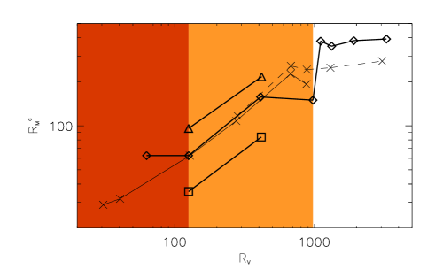
Figure 1: (Color online) Critical magnetic Reynolds $R_{M}^{c}$ as a function of $R_{V}$ for different Roberts flows (thick lines): $f=g$ ($\Diamond$), $f=g/\sqrt{2}$ ($\Box$), $f=g/0.77$ ($\triangle$). The dark (red) area corresponds to the region where the Roberts flow is hydrodynamically stable. For a comparison with Ref. Feudel et al. (2003), our Reynolds numbers should be divided by $2\pi$. The light (orange) area corresponds to the region of hydrodynamic oscillations, while the white area corresponds to the turbulent regime. The thin lines connected with crosses are shown as a reference and correspond to the threshold for dynamo instability in Taylor-Green flow Ponty et al. (2005): DNS (solid line) and $\alpha$-model (dashed line).

Figure 1 contains considerable information. There are basically three qualitative behaviors exhibited for different $R_{V}$, indicated by the (colored) background shading. For $R_{V}\lesssim 100$, the laminar Roberts flow is hydrodynamically steady-state and laminar, but dynamo action is still possible for large enough $R_{M}$. For $100\lesssim R_{V}\lesssim 1000$, Roberts flow treated purely hydrodynamically is temporally periodic but not turbulent. For $R_{V}\gtrsim 1000$, the Roberts flow develops a full turbulent spectrum hydrodynamically. In all three regimes, dynamo action is exhibited, but is different in the three regimes. The laminar regime was extensively studied in Ref. Feudel et al. (2003). Our definitions for the Reynolds numbers are different, but the results displayed in Figs. 1 and 2 are consistent with previous results in the range $P_{M}=[0.5,1]$ if our Reynolds numbers are divided by $2\pi$ (corresponding approximately to the integral scale of the laminar flow).

The threshold curve connecting diamonds ($\Diamond$) is for the Roberts flow with $f=g$ (helical, but not maximally so). The segment connecting squares ($\Box$) is for $f=g/\sqrt{2}$ (maximal helicity). The segment connected by triangles ($\triangle$) is for $f=g/0.77$, a less helical flow than $f=g$. The threshold curve connecting crosses ($\times$) is the threshold curve for the Taylor-Green (TG) flow from Ref. Ponty et al. (2005). All of these are direct numerical simulation (DNS) results. (We regard the fact that the Taylor-Green curve and the Roberts flow curve with $f=g$ have a common region above $R_{V}\sim 100$ to be coincidental). The curve connecting crosses ($\times$) with a dashed line is the result from Ref. Ponty et al. (2005) for the “$\alpha$-model”, or Lagrangian averaged model, of MHD.

Noteworthy in Fig. 1 is the qualitative similarity of the behavior of the threshold curve between the Roberts flow and the TG results from Ref. Ponty et al. (2005): a sharp rise in $R_{M}^{c}$ with the increase in the degree of turbulence in the velocity field, followed by a plateau in which further increases in $R_{V}$ show little effect upon $R_{M}^{c}$. It must be kept in mind that for both situations, the amplitude of the forcing field ${\bf f}$ is being adjusted so that $U$ and the total kinetic energy remain approximately constant, even though $R_{V}$ is increasing. Whether such a procedure corresponds to a physical driving force must be decided on a case-by-case basis.

Figure 2: Critical magnetic Reynolds $R_{M}^{c}$ as a function of $P_{M}^{-1}$ for the Roberts flow with $f=g$ (thick lines). The solid line corresponds to the laminar regime, the dashed line to the periodic flow, and the dotted line to the turbulent regime. (The double-valuedness results from the effects of two different values of $R_{V}$.)

Figure 2 shows the threshold curve for the Roberts flow with $f=g$ as a function of the inverse of the magnetic Prandtl number, $P_{M}^{-1}$. This curve shares some similarities with the TG flow, but also important differences. As in Ref. Ponty et al. (2005), between the laminar and turbulent regimes a sharp increase in $R_{M}^{c}$ is observed. Also, in the turbulent flow $R_{M}^{c}$ seems to be independent of the value of the magnetic Prandtl number. But while the TG force is not a solution of the Euler equations and was designed to generate smaller and smaller scale fluctuations as the Reynolds number $R_{V}$ is increased, the Roberts flow goes through several instabilities as $R_{V}$ is varied. As a result, the threshold for dynamo action in the $R_{M}$ vs. $P_{M}^{-1}$ plane is double-valued. For a given value of $P_{M}^{-1}$ two values of $R_{M}^{c}$ exist according to the hydrodynamic state of the hydrodynamic system, (e.g. laminar, periodic, or turbulent flow).

Figure 3: Kinetic energy spectra as a function of $R_{V}$. The Kolmogorov’s spectrum is showed as a reference.

Figure 4: Magnetic energy spectra during the kinematic regime, for different values of $R_{V}$. The values of $R_{M}$ for each curve correspond to the smallest value for which dynamo action was observed (see Fig. 5).

Figure 3 is a plot of the kinetic energy spectra for the values of $R_{V}$ shown in Fig. 1, for $f=g$, normalized so that $E_{V}(k=1)$ is unity for all cases. This is done to display the gradual widening of the spectrum as $R_{V}$ increases. Figure 4 shows corresponding magnetic spectra, normalized somewhat differently: the energy contained in the interval $1\leq k\leq 5$ is the same in all cases. This is done to emphasize the fact that the peak in the magnetic energy spectrum migrates to higher values as $R_{V}$ increases: the excited magnetic field develops more and more small-scale features. This may be related to the fact that because the forcing occurs at such low wavenumbers, inverse magnetic helicity cascades are effectively ruled out.

Figure 5: Growth rates as a function of $R_{M}$. Each line corresponds to several simulations at constant $R_{V}$ (fixed $\nu$), and each point in the line indicates the exponential growth (or decay) rate at a fixed value of $R_{M}$. The point where each curve crosses $\sigma=0$ gives the threshold $R_{M}^{c}$ for dynamo instability. $R_{V}=62.7$ ($\Box$), $R_{V}=125.5$ ($\times$), $R_{V}=416.2$ ($\triangle$), $R_{V}=974.4$ ($\Diamond$), $R_{V}=1108.1$ ($*$), $R_{V}=1327.7$ ($+$), $R_{V}=1912.5$ ($\circ$), and $R_{V}=3276.6$ ($\bigtriangledown$).

Figure 5 shows how the thresholds ($\sigma=0$) for the $R_{M}^{c}$ curves were calculated. For small initial $E_{M}$, broadly distributed over $k$, $\eta$ was gradually decreased in steps to raise $R_{M}$ in the same kinetic setting until a value of $\sigma\approx 0$ was identified. That provides a single point on such curves as those in Fig. 1.

Each simulation at a fixed value of $\nu$ and $\eta$ (or fixed $R_{V}$ and $R_{M}$) was extended for at least 100 large-scale turnover times to rule out turbulent fluctuations and obtain a good fit to the exponential growth. All the simulations were well-resolved and satisfied the condition $k_{\nu}/k_{max}<1$, where $k_{\nu}=(\epsilon/\nu^{3})^{1/4}$ is the Kolmogorov lengthscale, $\epsilon$ is the energy injection rate, $k_{max}=N/3$ is the largest resolved wavenumber, and $N$ is the linear resolution of the simulation. When this condition was not satisfied, the resolution $N$ was increased, from $N=64$ until reaching the maximum spatial resolution in this work of $256$ grid points in each direction, and a maximum mechanical Reynolds of $R_{V}=3276.6$.

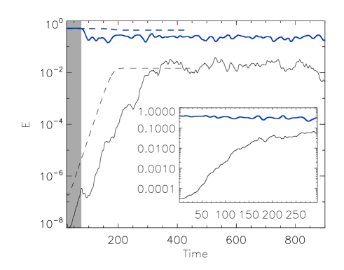
Figure 6: (Color online) Time history of the total kinetic [thick (blue) lines] and magnetic energy (thin lines) in dynamo simulations. The dashed lines correspond to $R_{V}=62.7$ and $R_{M}=78.4$ (laminar flow), while the solid lines are for $R_{V}=R_{M}=416.2$. The shaded region indicates the period of time when the flow is oscillating in this simulation. The inset shows the time history for a turbulent run with $R_{V}=3276.6$ and $R_{M}=1092.2$.

Figure 6 illustrates an interesting behavior that occurs when there is a transition from the laminar to the periodic regime of the Roberts flow ($f=g$). Figure 6 shows the evolution of total kinetic energies $E_{V}$ and magnetic energies $E_{M}$ for $R_{V}=62.7$ and $R_{V}=416.2$. The flat part of the kinetic [thick (blue)] curve for $R_{V}=416.2$ is characterized by small periodic oscillations too small to see on the logarithmic plot (they will be shown in Fig. 7). Meanwhile, the $E_{M}$ curve of magnetic energy is growing, somewhat irregularly. Rather suddenly, at about $t=70$, $E_{V}$ drops by more than a factor of 2 (see Fig. 7), and by $t\approx 300$ the magnetic energy has saturated at a level of about 1 per cent of the initial kinetic energy. Both fields oscillate irregularly after that, and are weakly turbulent. It is unclear how such a small magnetic excitation succeeds at shutting down such a large fraction of the flow. As will be shown later, this large drop is associated with the instability of the large scale flow. The inset shows the full time history of $E_{V}$ and $E_{M}$, for $R_{V}=3276.6$ and $R_{M}=1092.2$ when the turbulence is fully developed. The dashed line illustrates, for comparison, how simply the magnetic energy exponentiates and saturates in the laminar steady-state regime ($R_{V}=62.7$). Figure 7 shows in detail the suppression of the flow, manifested as a drop in the total energy, at $t\approx 70$.

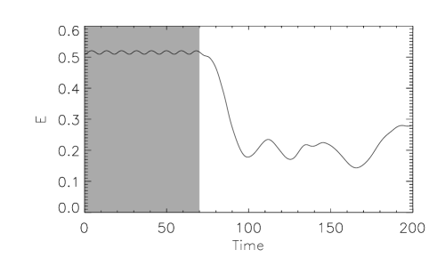
Figure 7: Time history of the total energy in the dynamo simulation with $R_{V}=R_{M}=416.2$. The shaded area is a blow up of the shaded region in Fig. 6 and corresponds to the hydrodynamic oscillations.

These oscillations between the hydrodynamic laminar and turbulent regime in the Roberts flow have been previously found by Feudel et al. Feudel et al. (2003). The authors pointed out that in this regime, close to the threshold $R_{M}^{c}$ the dynamo exhibits an intermittent behavior, with bursts of activity. The oscillatory flow is stable to small perturbations (e.g. numerical noise in the code), but as the magnetic energy grows the flow is perturbed by the Lorentz force and goes to a weakly turbulent regime. As noted in Ref. Feudel et al. (2003), if $R_{M}$ is close to $R_{M}^{c}$ then the magnetic field decays, the flow relaminarizes and the process is repeated. However, as observed in Fig. 6, if $R_{M}$ is large enough the weakly turbulent flow can still excite a dynamo, and the magnetic field keeps growing exponentially until reaching the non-linear saturation even after the hydrodynamic instability takes place.

Figure 8: Evolution of the magnetic energy in different shells in Fourier space: (a) $R_{V}=62.7$ and $R_{M}=78.4$ (laminar flow), (b) $R_{V}=R_{M}=416.2$ (periodic case), (c) $R_{V}=3276.6$ and $R_{M}=1092.2$ (turbulent regime). The dotted line corresponds to $k=1$, solid line to $k=2$, and the dashed lines to $k=9,10,11,12$.

Figure 8(a) shows the temporal growth of several Fourier components of the magnetic field in the laminar regime ($R_{V}=62.7$). A straightforward exponentiation, followed by a flat, steady-state, leveling-off exhibits the same growth rate for all harmonics. This indicates the existence of a simple unstable normal mode which saturates abruptly near $t\approx 180$. The behavior is much noisier for $R_{V}=416.2$ and $3276.6$ as shown in Figs. 8(b) and 8(c). Note that in the simulation with $R_{V}=416.2$, for $t<70$ all the magnetic modes oscillate with the same frequency as the hydrodynamic oscillations. In Figure 8, the dotted line and solid line above are, respectively, for $k=1$ and $k=2$. The remaining four are for $k=9$ through 11. The modes in between occupy the open space in between more or less in order. The same modes are shown for $R_{V}=416.2$ in Fig. 8(c), which illustrates a broad sharing of $E_{B}$ among many modes and a consequent excitation of small-scale magnetic components.

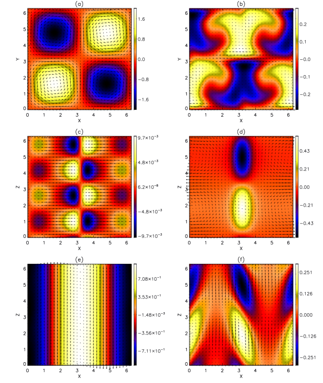
Figure 9: (Color online) Plots of the kinetic and magnetic fields for the saturated regime of the run with $R_{V}=62.7$ and $R_{M}=78.4$: (a) cut at $z=0$, $vz$ in color and $vx$, $vy$ indicated by arrows, (b) same as in (a) for the magnetic field, (c) cut at $y=0$, $vy$ in color and $vx$, $vz$ indicated by arrows, (d) same as in (c) for the magnetic field, (e) same as in (b) but for a cut at $y=\pi/4$, and (f) same as in (e) for the magnetic field.

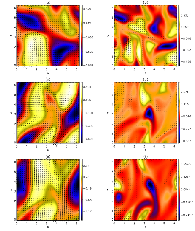
Figure 10: (Color online) Plots of the kinetic and magnetic fields for the saturated regime of the run with $R_{V}=R_{M}=416.2$. Labels and fields are as in Fig. 9.

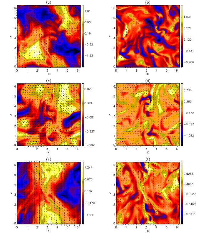
Figure 11: (Color online) Plots of the kinetic and magnetic fields for the saturated regime of the run with $R_{V}=3276.6$ and $R_{M}=1092.2$. Labels and fields are as in Fig. 9.

Plots of the kinetic and magnetic fields are shown in Figs. 9. The left column shows the velocity field in the saturated state for $R_{V}=62.7$, and the right column shows the magnetic field at the same time. The arrows indicate the vector components in the planes shown and the colors indicate the strengths of the perpendicular components. Figures 9(a) and (b) are for the plane $z=0$ and Figs. 9(c) and (d) are for the plane $y=0$. Figs. 9(e) and (f) are for the plane $y=\pi/2$. The velocity configuration shown in Fig. 9(a) is quite similar to the way it looks at $t=0$, but the $z$-dependences apparent in Figs. 9(c), (d), and (f) are not present in the initial flow.

Figs. 10 are similar color plots for the saturated regime for $R_{V}=416.2$. All the same quantities are being displayed at the same planes as in Figs. 9. The initial conditions are no longer recognizable in the saturated state, but is not yet sufficiently disordered that one would be forced to call it “turbulent”. Moreover, note that the four “cells” characteristic of the laminar Roberts flow [Fig. 9(a)] are not present in this late stage of the dynamo. During the early kinematic regime, when the hydrodynamic oscillations are observed, a slightly deformed version of these cells can be easily identified in the flow (not shown). When the magnetic energy grows due to dynamo action, the flow is unable to maintain this flow against the perturbation of the Lorentz force. This causes the large-scale flow to destabilize, and the kinetic energy in the shell $k=1$ drops by a factor of two. This instability of the large-scale modes is associated with the large drop of the kinetic and the total energy at $t\approx 70$ (Fig. 7).

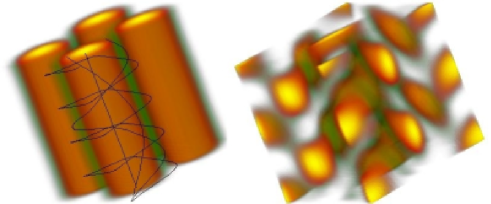
Figure 12: (Color online) Visualization of the kinetic (left) and magnetic energy density (right) for the saturated regime of the run with $R_{V}=62.7$ and $R_{M}=78.4$. Velocity field lines are indicated in black.

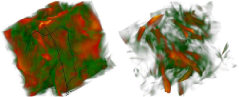
Figure 13: (Color online) Visualization of the kinetic (left) and magnetic energy density (right) for the saturated regime of the run with $R_{V}=3276.6$ and $R_{M}=1092.2$. Velocity field lines are indicated in black.

By contrast, the same fields are exhibited in the same planes in Figs. 11 in the saturated regime for $R_{V}=3276.6$. Here the truly turbulent nature of the flow is now apparent, particularly in the highly disordered magnetic field plots in the right-hand column.

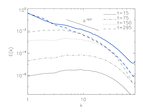
Figure 14: (Color online) Kinetic [thick (blue) line] and magnetic energy spectra for different times for the simulation with $R_{V}=3276.6$ and $R_{M}=1092.2$.

Figure 12 is a three-dimensional perspective plot of the kinetic and magnetic energy density for $R_{V}=62.7$ at a late time in the saturated regime. The kinetic energy distribution (on the left) is not much different than it was at $t=0$. The helical properties of the Roberts flow can be directly appreciated in the field lines indicated in black. In this regime, the flow is still laminar as previously indicated. The magnetic field is stretched and magnetic energy amplified in the four helical tubes, and then expelled out of the vortex tubes, accumulating in the stagnation points Roberts (1972); Feudel et al. (2003). Since the velocity field has no dependence in the $z$-direction, the magnetic field that can be sustained by dynamo action has to break this symmetry and displays a clear periodicity in this direction. The same energy densities are exhibited at a late time for the case of $R_{V}=3276.6$ in Fig. 13, and the highly filamented and disordered distributions characteristic of the turbulent regime are again apparent. Note however that still some helicity can be identified in the velocity field lines shown.

In Ref. Mininni et al. (2005a) a suppression of small scale turbulent fluctuations and an evolution of the system to a state with effective magnetic Prantdl number of order one was observed in the nonlinear saturation of the turbulent dynamo. Here a similar effect is observed, although the suppression of small scales is weaker probably due to the presence of the external forcing at $k\approx 1$ which does not leave room for a large scale magnetic field to develop. Figure 14 shows the time evolution of the kinetic and magnetic energy spectra in the run with $R_{V}=3276.6$ and $R_{M}=1092.2$. While at early times the magnetic energy spectrum peaks at small scales ($k\approx 9$), at late times the magnetic spectrum is flat for small $k$ and drops together with the kinetic energy. The kinetic spectrum is strongly quenched and has a large drop at small scales.

IV SUMMARY AND DISCUSSION

One apparent outcome of these computations has been to confirm the intuitive impression that dynamo amplification of very small magnetic fields in conducting fluids is easier if mechanical helicity is present. This is true in velocity fields which are both turbulent and laminar. The values of $R_{M}^{c}$ which are the lowest found ($\sim 10$) are well below those in several existing experimental searches.

It is also somewhat reassuring to find that the qualitative behavior of dynamo thresholds with decreasing viscosity (increasing Reynolds number at fixed $U$) is as similar as it is to that found for the non-helical TG flow in Ref. Ponty et al. (2005). In particular, since the simulations discussed here were forced at almost the largest scale available in the periodic domain, a turbulent regime for $P_{M}<1$ where $R_{M}^{c}$ is approximately independent of $P_{M}$ was reached using only DNS, while for the TG flow two different models Mininni et al. (2005b); Ponty et al. (2004) for the small scales were needed. The similarities in the behavior of the threshold for the two flows for $P_{M}$ small enough brings more confidence to the ability of subgrid scale models of MHD turbulence to predict results in regimes of interest for astrophysics and geophysics that are today out of reach using DNS. That being said, it should be admitted that the Roberts flow in a way exhibits a richer set of possibilities in that the dynamo activity is somewhat different in each of the three regimes (laminar and steady-state, oscillatory, and turbulent).

Dynamo action is to be regarded as of many types Mininni et al. (2005a) and situation-dependent. The forms of the magnetic fields developed and their characteristic dimensions are determined to a considerable extent by the mechanical activity that excites them and by the geometric setting in which they take place. If it is desired to apply the theoretical and computational results to planetary dynamos or laboratory experiments, then rectangular periodic conditions appear to be a constraint that should be dispensed with as soon as feasible.