Solving procedure for a twenty-five diagonal coefficient matrix: direct numerical solutions of the three dimensional linear Fokker-Planck equation

Abstract

We describe an implicit procedure for solving linear equation systems resulting from the discretization of the three dimensional (seven variables) linear Fokker-Planck equation. The discretization of the Fokker-Planck equation is performed using a twenty-five point molecule that leads to a coefficient matrix with equal number of diagonals. The method is an extension of Stone’s implicit procedure, includes a vast class of collision terms and can be applied to stationary or non stationary problems with different discretizations in time. Test calculations and comparisons with other methods are presented in two stationary examples, including an astrophysical application for the Miyamoto-Nagai disk potential for a typical galaxy.

I Introduction

In dealing with solutions of partial differential equations we often encounter a set of linear equations that has to be solved. This set of linear equations depends on the method used for discretization. In general, when dealing with three dimensional systems the number of linear equations increases and the numerical solution of these equations uses most of the computing time. An extreme case is the Fokker-Planck equation. The Fokker-Planck equation is also known as the Fokker-Planck approximation because truncates the BBGKY (N.N. Bogoliubov, M. Born, H.S. Green, J.G. Kirkwood, and J. Yvon) hierarchy of kinetic equations at its lowest order by assuming that correlation between particles only plays a role as a sequence of uncorrelated two-body encounters rei ; hua . Note that the only “approximation” made in the Fokker-Planck equation comes from the model adopted for collisions and, in fact, the Fokker-Planck equation can be derived from first principles and no ad hoc suppositions are needed. The solution of the Fokker-Planck equation equation is not an easy task because in the three dimensional case it has seven variables: three space coordinates (x), three velocity coordinates (v) and time ($t$). In the two dimensional case there is a simplification because the total number of variables are five. In either case, the large number of grid nodes needed for the computation of the solution becomes a storage data problem. In a three dimensional problem, for a stationary or non stationary equation, the number of linear equations corresponds to the number of nodes in the phase-space grid (x,v). If we divide each of the phase-space variables’ interval of the distribution function in nine parts (ten nodes), we will have a grid with $10^{6}$ nodes. In a simple numerical method we have to store and solve a matrix with $10^{12}$ elements. For the two dimensional case, the main matrix will have $10^{8}$ elements. With 10 grid nodes per variable only very simple geometries can be described. The large number of matrix elements brings us another computational problem, the slowness of the codes. In the discretization process of the Fokker-Planck equation, a system of linear equations is obtained and arranged into a matrix form (coefficient matrix). For the case of a finite difference scheme discretization in three dimensions with a twenty five point molecule, we see that approximately less than 0.003% of the elements are different from zero. This incentives us to search for alternative and faster methods, usually iterative, to solved the linear system using only the non null data. Note that, in general, the coefficient matrix is not symmetric. So, powerful methods like the Conjugate Gradient hes:sti ; ger:whe and Cholesky ger:whe decomposition can not be used. Our main goal is to obtain a code that allows us to obtain a fast and effective numerical solutions on high resolution schemes of the three dimensional linear Fokker-Planck equation in a direct way. The importance and difficulties of having three dimensional solutions of the Fokker-Planck equation can be summarized in the words of Binney and Tremaine (bin:tre page 245), here in relation with galactic dynamics: Finding the particular function of three variables that describes any given galaxy is no simple matter. In fact, this task has proved so daunting that only in the last few years, three-quarters of a century after Jeans’s (Jeans jea ) paper posed the problem, has the serious quest for the distribution function of even our own Galaxy got underway.

We mean by direct numerical calculations of the Fokker-Planck equation a method that is neither statistical nor mean field approximation bin:tre . Numerical solutions can be performed using statistical approximate methods like the method of moment equations lar1 ; lar2 ; lyn:egg and Monte Carlo methods hen1 ; hen2 . Also, solutions have been found using the orbit-averaged Fokker-Planck equation with action-angle variables bin:tre , this last method reduces the equation involving six phase-space coordinates plus time to one involving only three actions plus time. Another method that have been used for solving the Vlasov equation with good results is the operator splitting technique che:kno ; gag:sho . Two dimensional numerical integration of the Vlasov equations can be found in sho:ger . The problem associated with this method is that, even in the two dimensional case, the time spent in making the interpolation is very expensive. Direct three dimensional numerical calculations of the Fokker-Planck equations, to the best of our knowledge, has not been done. As we said before, the main difficulty to find the solution of the three dimensional Fokker-Planck equation is the large number of linear equations that is translated in a high computational cost involve in the process. In this article we present a variations of Stone’s sto method that leads us to solve with low computational cost the three dimensional linear Fokker-Planck equation. Variations of Stone’s method has been applied to other situations in two sch:zed and three lei:per space dimensions when dealing with fluid flow, heat transfer and Laplace equation.

In this article we study how to solve the system of equations that arises from the discretization process using a finite difference scheme, in particular we used a twenty-five point molecule, but we have to keep in mind that other discretization procedures gives practically the same form for the coefficient matrix and this method can also be applied, i.e. sparse matrices with the same number of diagonals. For example, in two dimensions, the diffusion equation can be discretized in an uniform rectangular grid by using the finite difference scheme, the finite volume method (which is a discretization of the equation in integral form) or the finite element method, see fle . All of these methods gives five diagonals, in the finite element method the number of diagonals depends on the type of interpolation considered, and the coefficient matrix can be solved by the same numerical method. So, in this article, we shall not discuss what discretization method is better for the problem considered, we rather present a numerical method that allows us to find the solution of a coefficient matrix with twenty-five diagonals that can be obtained with different discretization methods.

The article is organized as follows. In Section II we present the linear Fokker-Planck equation to be solved. We consider a linear collision term that includes a vast class of collisions. In Section III, we describe the algorithm of the modified Stone method to obtain the incomplete $LU$ decomposition. The discretization of the Fokker-Planck equation is performed using a central difference approximation for the phase-space variables (x,v) that is described with a twenty-five point molecule. This point molecule also allows to describe different discretizations in time, as the implicit Euler or Crank-Nicolson discretization. The derivation of the $LU$ decomposition is made without assuming any particular discretization in time, maintaining its derivation as general as possible. The notation used for the diagonals in the coefficient matrix is also shown. In Section IV, we test our algorithm with an astrophysical example by solving the Fokker-Planck equation for the widely used Miyamoto-Nagai disk potential miy:nag in three dimensions. The parameters of the model are chosen to represent the Newtonian potential of a typical galaxy. Also, we used a Fokker-Planck test equation to compare our algorithm with the Generalized Minimal Residual Method (GMRES) that solves large sparse matrices. In Section V, we show how to modified the code to implement curved boundary conditions. Finally, in Section VI, we summarized our results.

II The general problem

The linear Fokker-Planck equation can be written as

$$\frac{\partial f}{\partial t}+{\bf v}\cdot\nabla f+\dot{\bf v}\cdot\nabla_{v}f=\Gamma[f],$$ (1)

where ${\bf v}$ represent the velocity of the particles, $\nabla$ is the usual gradient, $\nabla_{v}$ is the velocity gradient (derivations are done with respect to the velocities), $\dot{\bf v}$ is the acceleration and the symbol $\Gamma[f]$ denotes the rate of change of $f$ due to encounters (collision term). We consider as the collision term the expression

$$\Gamma[f]=A({\bf x,v})\nabla^{2}f+B({\bf x,v})\nabla^{2}_{v}f+C({\bf x,v})\nabla f+D({\bf x,v})\nabla_{v}f+\sum_{i\neq j=1}^{3}E_{ij}({\bf x,v})\frac{\partial^{2}f}{\partial v_{i}\partial v_{j}},$$ (2)

where $A$, $B$, $C$, $D$ and $E_{ij}$ are arbitrary functions of the phase-space variables ${\bf x}$ and ${\bf v}$. The equation above describes a vast family of collisions. In particular, with the mixed velocity derivative term present in (2) we can take into account the important collision term found by Rosenbluth et al. ros:mac used in gravitating systems and plasma physics, see for example ein:spu ; gal:mac and nan ; bro:pre respectively, and reference therein. If we need mixed space derivatives instead of mixed velocity derivatives, we can use the same code presented in this article to solve the problem. If a particular problem requires the inclusion of mixed velocity derivatives as well as mixed space derivatives, it is possible to develop a similar numerical procedure following the steps of this article, but it complicates the incomplete $LU$ decomposition used for the method, i.e. we need twelve extra diagonals on the coefficient matrix (thirty-seven instead of twenty-five diagonals).

In Section IV we solve numerically the stationary linear Fokker-Planck equation (1). In general, Eq. (1) is non-linear because $\dot{\bf v}={\bf F}(f)/m$, where ${\bf F}$ is the force and $m$ is the mass of the particle. Another kind of non-linearity may arrise from the collision term considered. A way to deal with this kind of problem is to start with a given distribution function at time $t$ from which we can calculate the force and collision term at this time. Then, this force and collision term are replaced into the Fokker-Planck equation from which we obtain the distribution function for a later time $t+\Delta t$. With the recently calculated distribution function we can calculate again the force and collision term at time $t+\Delta t$ and the process is repeated. An application for a stationary non-linear problem can be found in uje:let , in which we found the distribution function that satisfies both Fokker-Planck and Poisson equation in two dimensions for a Kuzmin-Toomre thin disk.

Table 1: Nomenclature and relations between the matrix form and the one dimensional storage index at node $p$ of the twenty-five terms used in the discretization of the Fokker-Planck equation.

Matrix Form	Abbreviation	Name	Position From Node $p$
	Basic Diagonals
$\Psi(i,j,k,l,m,n)$	$P$	point	$p$
$\Psi(i,j+1,k,l,m,n)$	$N$	north	$p+1$
$\Psi(i,j-1,k,l,m,n)$	$S$	south	$p-1$
$\Psi(i+1,j,k,l,m,n)$	$E$	east	$p+n_{j}$
$\Psi(i-1,j,k,l,m,n)$	$W$	west	$p-n_{j}$
$\Psi(i,j,k+1,l,m,n)$	$T$	top	$p+n_{ij}$
$\Psi(i,j,k-1,l,m,n)$	$B$	bottom	$p-n_{ij}$
$\Psi(i,j,k,l+1,m,n)$	$U1$	up1	$p+n_{ijk}$
$\Psi(i,j,k,l-1,m,n)$	$D1$	down1	$p-n_{ijk}$
$\Psi(i,j,k,l,m+1,n)$	$U2$	up2	$p+n_{ijkl}$
$\Psi(i,j,k,l,m-1,n)$	$D2$	down2	$p-n_{ijkl}$
$\Psi(i,j,k,l,m,n+1)$	$U3$	up3	$p+n_{ijklm}$
$\Psi(i,j,k,l,m,n-1)$	$D3$	down3	$p-n_{ijklm}$
	Mixed Diagonals
$\Psi(i,j,k,l+1,m+1,n)$	$UT2$	uptop2	$p+(n_{ijkl}+n_{ijk})$
$\Psi(i,j,k,l-1,m+1,n)$	$UB2$	upbottom2	$p+(n_{ijkl}-n_{ijk})$
$\Psi(i,j,k,l+1,m-1,n)$	$DT2$	downtop2	$p-(n_{ijkl}-n_{ijk})$
$\Psi(i,j,k,l-1,m-1,n)$	$DB2$	downbottom2	$p-(n_{ijkl}+n_{ijk})$
$\Psi(i,j,k,l+1,m,n+1)$	$UT3$	uptop3	$p+(n_{ijklm}+n_{ijk})$
$\Psi(i,j,k,l-1,m,n+1)$	$UB3$	upbottom3	$p+(n_{ijklm}-n_{ijk})$
$\Psi(i,j,k,l+1,m,n-1)$	$DT3$	downtop3	$p-(n_{ijklm}-n_{ijk})$
$\Psi(i,j,k,l-1,m,n-1)$	$DB3$	downbottom3	$p-(n_{ijklm}+n_{ijk})$
$\Psi(i,j,k,l,m+1,n+1)$	$UU3$	upup3	$p+(n_{ijklm}+n_{ijkl})$
$\Psi(i,j,k,l,m-1,n+1)$	$UD3$	updown3	$p+(n_{ijklm}-n_{ijkl})$
$\Psi(i,j,k,l,m+1,n-1)$	$DU3$	downup3	$p-(n_{ijklm}-n_{ijkl})$
$\Psi(i,j,k,l,m-1,n-1)$	$DD3$	downdown3	$p-(n_{ijklm}+n_{ijkl})$

III Description of the algorithm

The system of equations obtained from the discretization of the Fokker-Planck equation (1,2) using the central finite difference approximation for the phase-space and a temporal discretization in time (implicit Euler, Crank-Nicolson, etc.) can be cast (for each time step) into the simple form,

$$A\Psi=Q,$$ (3)

in which $A$ is a square coefficient matrix $N_{node}\times N_{node}$ ($N_{node}$ the number of nodes in the discretization grid), $\Psi$ is the vector matrix of the nodal variable values, and $Q$ is the source vector. The position of the grid nodes in the phase-space ($x,y,z,v_{x},v_{y},v_{z}$) is performed by six indexes ($i,j,k,l,m,n$), where $i$ represents the index for the variable $x$, $j$ represents the index for the variable $y$, etc. The ordering of nodes in this six dimensional space is made as follows. The surface $n$=constant are stacked one above another. Within the fifth dimensional space (for each $n$) the hyper-surfaces $m$=constant are stacked one above another. Within the fourth dimensional space (for each $n$ and $m$) the hyper-surfaces $l$=constant are stacked one above another. Within the three dimensional space (for each $n$, $m$ and $l$) the surfaces $k$=constant are stacked one above another. Within the two dimensional space (for each $n$, $m$, $l$ and $k$) the index $j$ increases first ($y$-direction) than the index $i$ ($x$-direction). The one dimensional storage index $p$ of the vector matrix $\Psi$ is calculated from the six-dimensional grid indexes ($i,j,k,l,m,n$), i.e.

$$p=(n-1)n_{ijklm}+(m-1)n_{ijkl}+(l-1)n_{ijk}+(k-1)n_{ij}+(i-1)n_{j}+j,$$ (4)

with

$$i=1\cdots n_{i};\;\;j=1\cdots n_{j};\;\;k=1\cdots n_{k};\;\;l=1\cdots n_{l};\;\;m=1\cdots n_{m};\;\;n=1\cdots n_{n};$$

$$n_{ijklm}=n_{i}n_{j}n_{k}n_{l}n_{m};\;\;n_{ijkl}=n_{i}n_{j}n_{k}n_{l};\;\;n_{ijk}=n_{i}n_{j}n_{k};\;\;n_{ij}=n_{i}n_{j};$$ (5)

Figure 1: Form of the coefficient matrix $A$ obtained from the discretization of the partial difference equation of our problem. The separation between the main diagonal $P$ and the other diagonals are indicated. Also, the distance between the diagonals of the mixed derivatives to their nearest diagonals are shown. Note that the figure is not in scaled.

Figure 2: Schematic representation of the matrices $L$, $U$ and their product $M$. The multiplication of the matrices $L$ and $U$ leads to extra diagonals (dotted lines) not present in the coefficient matrix $A$. The diagonals of $L$, from the left-bottom corner to the main diagonal, are: $DD3$, $DB3$, $D3$, $DT3$, $DU3$, $DB2$, $D2$, $DT2$, $D1$, $W$, $S$, $P$. The diagonals of $U$, from the main diagonal to the right-up diagonal, are: $1$, $N$, $E$, $T$, $U1$, $UB2$, $U2$, $UT2$, $UD3$, $UB3$, $U3$, $UT3$, $UU3$. The diagonals in $M$ are products of these two sets of diagonals but we have to be careful because more than one product can be at the same diagonal.

where $n_{i}$, $n_{j}$, $n_{k}$, $n_{l}$, $n_{m}$, $n_{n}$ denote the number of grid points for each variable. Therefore $N_{node}=n_{i}n_{j}n_{k}n_{l}n_{m}n_{n}$. With the help of the storage index $p$ we can switch each point of the twentyfive-point molecule from the matrix form to the one dimensional position representation. This is done in Table 1 by making the equivalence $f(x,y,z,v_{x},v_{y},v_{z})\equiv\Psi(i,j,k,l,m,n)$. Until now, we considered only the non stationary case, but the discretization in Table 1 can be used in the non stationary as well as the stationary Fokker-Planck equation. In both cases, the final system of equations is of the form (3), with $A$ being a sparse matrix with elements different from zero in only twenty-five diagonals, see Fig. 1. Now, we want to develop an iteration method in order to solve the system of equations (3). After $h$ iterations of such method, the approximate solution $\Psi^{h}$ do not satisfies (3) exactly, their is a non zero residual $R$ such as

$$A\Psi^{h}=Q-R^{h}.$$ (6)

The purpose of the iteration procedure is to drive the residual term to zero after some number of iteration (actually we stop the iteration when the residual term attained some imposed small value condition). Let us consider an iterative scheme for a linear system in the form

$$M\Psi^{h+1}=O\Psi^{h}+B,$$ (7)

when convergence is achieved we must have that $A=M-O$ and $B=Q$. An alternative version of this procedure can be obtained by subtracting $M\Psi^{h}$ from both sides of (7) to have,

$$M\Delta^{h+1}=R^{h},$$ (8)

where $\Delta^{h+1}=\Psi^{h+1}-\Psi^{h}$ and $R^{h}=B-(M-O)\Psi^{h}=Q-A\Psi^{h}$. Any effective iterative method to solve (7) must be cheap and converge rapidly. For faster convergence, the matrix $M$ have to be a good approximation of the coefficient matrix $A$, i.e. we must have $O\Psi^{h}$ small. The original idea of Stone is to use for the iteration matrix $M$ an incomplete $LU$ decomposition of the matrix $A$. The reason for this choice is that $LU$ decomposition is an excellent linear system solver. The matrices $L$ and $U$ have elements different from zero only in the diagonals in which $A$ have also elements different from zero. The product of the matrices, $L$ and $U$, provide a matrix $M$ with a larger number of diagonals with elements different from zero, see for instance Fig. 2. To make the decomposition $LU$ unique, we set the elements on the principal diagonal of $U$ equal to 1. In doing the $LU$ multiplication, we have to pay extra attention because sometimes more than one diagonal product are at the same distance from the main diagonal $P$, e.g. the product $L_{D3}\cdot U_{1}$ and $L_{DD3}\cdot U_{U2}$ are at the same diagonal in $M$. The multiplication rules for matrices furnish the elements of $M=LU$ at node $p$ (see Appendix A), where for example, $M_{W|UU3}$ represents the diagonal in $M$ that is obtain from the multiplication between the elements of the diagonal $S$ in $L$ with the elements of the diagonal $UU3$ in $U$.

Now, we choose $L$ and $U$ in such a way that $M(=A+O)$ is the best possible approximation to $A$. The standard method for decomposition is to let $O$ to have elements different from zero in the diagonals of $M$ that corresponds to the diagonals not present in $A$ and to force the other diagonals of $M$ to be equal to the corresponding diagonals in $A$. But this method converges slowly because the resulting matrix $O$ is not small. Stone recognized that the convergence of the method could be faster if we allow $O$ to have elements different from zero also in the diagonals present in $A$. The key idea is that the contribution of $M\Psi$ of the diagonals not present in $A$ partially canceled the contribution of $O\Psi$ of the diagonals present in $A$, in such a way that

$$O\Psi\approx 0.$$ (9)

Note that in (24) they are diagonals in $M$ that present more than one term. In general, the principal diagonals have more than one element, as for example $M_{DT3}$, but beside these principal diagonals there are other no-principal diagonals that have more than one element, like $M_{D3|UB2}$. Now, relation (9) can be written for one grid node in several ways. The usual way is to consider the elements of these no-principle diagonals as part of the same diagonal. Other way is to consider these elements as they were from different diagonals, thus in this case, following the above example, the no-principal diagonal $M_{D3|UB2}$ is split into two diagonals $M_{D3|UB2}$ and $M_{DB3|U2}$. We obtained the final relations for the $LU$ decomposition in both ways and we found that the $LU$ decomposition considering the elements as they were from different diagonals is faster by a factor of two. Hereafter we consider this case. The explicit form of equation (9) is given in Appendix B.

The problem now is to defined the elements of $O$ to satisfy Eq. (25) without introducing additional unknowns. If we expect the solution of the partial differential equation to be smooth, we can approximate the values of $\Psi_{B|N}$, $\Psi_{N|W}$, etc, in terms of the values of $\Psi$ at nodes corresponding to the diagonals of A. Stone proposed the following approximations (other approximations are possible),

$$\Psi_{B|N}\approx\alpha(\Psi_{B}+\Psi_{N}-\Psi_{P}),$$

$$\Psi_{W|N}\approx\alpha(\Psi_{W}+\Psi_{N}-\Psi_{P}),\;{\rm etc}$$ (10)

where $\alpha$ is a constant. Stability analysis made by Stone requires that $\alpha$ must be between $0<\alpha<1$. Replacing the above approximations into (25) we obtain the elements of $O$ as a linear combination of the elements of $M$, see for instance Appendix C. Now, using the relation $M=A+O$ together with expressions (24) and (26), we find that the elements of the matrices $L$ and $U$ are given by,

$$L_{[X]}^{p}=\frac{A_{[X]}^{p}-C_{[X]}}{1+\alpha K_{[X]}},\;\;\;[X]=DD3,\;DB3,\;D3,\;DT3,\;DU3,\;DB2,\;D2,\;DT2,\;D1,\;B,\;W,\;S,$$

$$L_{P}^{p}=A_{P}^{p}-L_{S}^{p}U_{N}^{p-1}-L_{W}^{p}U_{E}^{p-n_{j}}-L_{B}^{p}U_{T}^{p-n_{ij}}-L_{D1}^{p}U_{U1}^{p-n_{ijk}}-L_{DT2}^{p}U_{UB2}^{p-(n_{ijkl}-n_{ijk})}-L_{D2}^{p}U_{U2}^{p-n_{ijkl}}$$

$$\hskip 28.45274pt-L_{DB2}^{p}U_{UT2}^{p-(n_{ijkl}+n_{ijk})}-L_{DU3}^{p}U_{UD3}^{p-(n_{ijklm}-n_{ijkl})}-L_{DT3}^{p}U_{UB3}^{p-(n_{ijklm}-n_{ijk})}-L_{D3}^{p}U_{U3}^{p-n_{ijklm}}$$

$$\hskip 28.45274pt-L_{DB3}^{p}U_{UT3}^{p-(n_{ijklm}+n_{ijk})}-L_{DD3}^{p}U_{UU3}^{p-(n_{ijklm}+n_{ijkl})}+\alpha(K_{N}+K_{E}+K_{T}+K_{U1}+K_{UB2}+K_{U2}+K_{UT2}$$

$$\hskip 28.45274pt+K_{UD3}+K_{UB3}+K_{U3}+K_{UT3}+K_{UU3}),$$

$$U_{[X]}^{p}=\frac{A_{[X]}^{p}-\alpha K_{[X]}-C_{[X]}}{L_{P}^{p}},\;\;\;[X]=N,\;E,\;T,\;U1,\;UB2,\;U2,\;UT2,\;UD3,\;UB3,\;U3,\;UT3,\;UU3,$$ (11)

where the explicit form of the functions $C_{[X]}$ and $K_{[X]}$ are given in the Appendix D. The elements of the $LU$ decomposition have to be calculated in the order specified in (11). In doing this, we must take into account that a certain element is considered equal to zero if its storage index is less or equal zero, e.g. if $p=3$ and $n_{j}=5$ then the elements with index $p$ and $p-1$ are different from zero, and the elements with index $p-n_{j}$, $p-n_{ij}$, etc are equal to zero. When mixed derivatives are not present we must set all the elements with index $DD3$, $DB3$, $DT3$, $DU3$, $DB2$, $DT2$, $UB2$, $UT2$, $UD3$, $UB3$, $UT3$, $UU3$ equal to zero. Once obtained the $LU$ decomposition, the system of equation is solved combining $M=LU$ with (8) to obtain

$$LU\Delta^{h+1}=R^{h},$$ (12)

and here we set

$$L\Upsilon^{h}=R^{h},$$

$$U\Delta^{h+1}=\Upsilon^{h},$$ (13)

from which we obtain the solution of our problem by solving two triangular systems. In this iterative method, the matrix elements of $L$ and $U$ are calculated only once before the first iteration. In other iterations, only the residual $R$, $\Upsilon$ and $\Delta$ are calculated using the two triangular system mentioned above, i.e.,

$$\Upsilon^{p}=(R^{p}-L^{p}_{DD3}\Upsilon^{p-(n_{ijklm}+n_{ijkl})}-L^{p}_{DB3}\Upsilon^{p-(n_{ijklm}+n_{ijk})}-L^{p}_{D3}\Upsilon^{p-n_{ijklm}}-L^{p}_{DT3}\Upsilon^{p-(n_{ijklm}-n_{ijk})}$$

$$\hskip 28.45274pt-L^{p}_{DU3}\Upsilon^{p-(n_{ijklm}-n_{ijkl})}-L^{p}_{DB2}\Upsilon^{p-(n_{ijkl}+n_{ijk})}-L^{p}_{D2}\Upsilon^{p-n_{ijkl}}-L^{p}_{DT2}\Upsilon^{p-(n_{ijkl}-n_{ijk})}-L^{p}_{D1}\Upsilon^{p-n_{ijk}}$$

$$\hskip 28.45274pt-L^{p}_{B}\Upsilon^{p-n_{ij}}-L^{p}_{W}\Upsilon^{p-n_{j}}-L^{p}_{S}\Upsilon^{p-1})/L^{p}_{P},$$

$$\Delta^{p}=\Upsilon^{p}-U^{p}_{UU3}\Delta^{p+(n_{ijklm}+n_{ijkl})}-U^{p}_{UT3}\Delta^{p+(n_{ijklm}+n_{ijk})}-U^{p}_{U3}\Delta^{p+n_{ijklm}}-U^{p}_{UB3}\Delta^{p+(n_{ijklm}-n_{ijk})}$$

$$\hskip 28.45274pt-U^{p}_{UD3}\Delta^{p+(n_{ijklm}-n_{ijkl})}-U^{p}_{UT2}\Delta^{p+(n_{ijkl}+n_{ijk})}-U^{p}_{U2}\Delta^{p+n_{ijkl}}-U^{p}_{UB2}\Delta^{p+(n_{ijkl}-n_{ijk})}-U^{p}_{U1}\Delta^{p+n_{ijk}}$$

$$\hskip 28.45274pt-U^{p}_{T}\Delta^{p+n_{ij}}-U^{p}_{E}\Delta^{p+n_{j}}-U^{p}_{N}\Delta^{p+1},$$ (14)

where

$$R^{p}=Q^{p}-A_{P}^{p}\Psi^{p}-A_{N}^{p}\Psi^{p+1}-A_{S}^{p}\Psi^{p-1}-A_{E}^{p}\Psi^{p+n_{j}}-A_{W}^{p}\Psi^{p-n_{j}}-A_{T}^{p}\Psi^{p+n_{ij}}-A_{B}^{p}\Psi^{p-n_{ij}}-A_{U1}^{p}\Psi^{p+n_{ijk}}$$

$$\hskip 28.45274pt-A_{D1}^{p}\Psi^{p-n_{ijk}}-A_{UB2}^{p}\Psi^{p+(n_{ijkl}-n_{ijk})}-A_{DT2}^{p}\Psi^{p-(n_{ijkl}-n_{ijk})}-A_{U2}^{p}\Psi^{p+n_{ijkl}}-A_{D2}^{p}\Psi^{p-n_{ijkl}}$$

$$\hskip 28.45274pt-A_{UT2}^{p}\Psi^{p+(n_{ijkl}+n_{ijk})}-A_{DB2}^{p}\Psi^{p-(n_{ijkl}+n_{ijk})}-A_{UD3}^{p}\Psi^{p+(n_{ijklm}-n_{ijkl})}-A_{DU3}^{p}\Psi^{p-(n_{ijklm}-n_{ijkl})}$$

$$\hskip 28.45274pt-A_{UB3}^{p}\Psi^{p+(n_{ijklm}-n_{ijk})}-A_{DT3}^{p}\Psi^{p-(n_{ijklm}-n_{ijk})}-A_{U3}^{p}\Psi^{p+n_{ijklm}}-A_{D3}^{p}\Psi^{p-n_{ijklm}}$$

$$\hskip 28.45274pt-A_{UT3}^{p}\Psi^{p+(n_{ijklm}+n_{ijk})}-A_{DB3}^{p}\Psi^{p-(n_{ijklm}+n_{ijk})}-A_{UU3}^{p}\Psi^{p+(n_{ijklm}+n_{ijkl})}-A_{DD3}^{p}\Psi^{p-(n_{ijklm}+n_{ijkl})},$$

in which, for simplicity, we have omitted the iterative index $h$.

IV Test results and comparisons with other methods

As was mentioned in the Introduction, the huge number of nodes needed to solve the Fokker-Planck equation leads to large amount of data that has to be stored in a matrix, this fact reduces the possible codes for testing the results. Furthermore, in general, the Fokker-Planck equation (1) is not symmetric, and for that reason other methods can not be used. In this case, the Generalized Minimal Residual method (GMRES) saa:sch is the most appropriate choice. The GMRES method belongs to the class of Krylov based iterative methods lan1 ; arn ; lan2 and was proposed in order to solve large, sparse and non Hermitian linear systems. This section is divided into two parts. In the first part, we apply the method presented in this article to a physical example. In particular, we choose the astrophysical problem of finding the distribution function of the Miyamoto-Nagai disk in three dimensions. In the second part, we used a simplified version of the physical example to make numerical comparisons. We compare our method with the best available method in solving huge sparse matrices, i.e. GMRES. We prefer to make the numerical comparisons with the simplified version of the physical example because the large amount of parameters present in the physical example make the analysis cumbersome. This analysis is important because we show some advantages and limitations of our method.

IV.1 Physical Example

To test of our code we begin with an important astrophysical application, i.e. solve the Fokker-Planck equation to find the distribution function of the Miyamoto-Nagai disk miy:nag in three dimensions in a stationary regime. The Fokker Planck equation to be solved is bin:tre

$${\bf v}\cdot\nabla f+\dot{\bf v}\cdot\nabla_{v}f=-\sum_{i=1}^{3}\frac{\partial}{\partial v_{i}}[f({\bf x,v})D(\Delta v_{i})]+\frac{1}{2}\sum_{i,j=1}^{3}\frac{\partial^{2}}{\partial v_{i}\partial v_{j}}[f({\bf x,y})D(\Delta v_{i}\Delta v_{j})],$$ (15)

where $\dot{\bf v}=-\nabla\Phi$, $\Phi=-\frac{GM}{\sqrt{x^{2}+y^{2}+(a+\sqrt{z^{2}+b^{2}})^{2}}}$, $G$ is the gravitational constant, $M$ is the total mass of the system, $a$ and $b$ are parameters that depending on the choice the potential can represent anything from an infinitesimal thin disk to a spherical system, and the functions $D(\Delta v_{i})$ and $D(\Delta v_{i}\Delta v_{j})$ are known as the diffusion coefficients. These diffusion coefficients were calculated by Rosenbluth et al. ros:mac considering a test star of mass $m$ moving through an infinite homogeneous sea of field stars of mass $m_{a}$ who has mean velocity equal to zero. Moreover, the interaction between the particles are ruled by an inverse square force, and also, each stellar encounter involve only a single pair of stars and are independent of all others. These diffusion coefficients are simplified if the field stars distribution function is a Maxwellian distribution. The explicit form of these coefficients are bin:tre .

$$D(\Delta v_{i})=\frac{v_{i}}{v}D(\Delta v_{||}),$$ (16)

$$D(\Delta v_{i}\Delta v_{j})=\frac{v_{i}v_{j}}{v^{2}}[D(\Delta v^{2}_{||})-\frac{1}{2}D(\Delta v^{2}_{\bot})]+\frac{1}{2}\delta_{ij}D(\Delta v^{2}_{\bot}),$$ (17)

where $D(\Delta v_{||})$, $D(\Delta v^{2}_{||})$ and $\Delta v^{2}_{\bot}$ are given by

$$D(\Delta v_{||})=-\frac{4\pi G^{2}\rho(m+m_{a})\ln\Lambda{\rm G}(X)}{\sigma^{2}},$$ (18)

$$D(\Delta v^{2}_{||})=\frac{4\sqrt{2}\pi G^{2}\rho m_{a}\ln\Lambda}{\sigma}\frac{{\rm G}(X)}{X},$$ (19)

$$D(\Delta v^{2}_{\bot})=\frac{4\sqrt{2}\pi G^{2}\rho m_{a}\ln\Lambda}{\sigma}\left[\frac{{\rm erf}(X)-{\rm G}(X)}{X}\right],$$ (20)

Figure 3: Numerical solutions of the distribution function of Eq. (15). Top: surface distribution for the case with $v_{x}\approx-117$ km s^-1, $v_{y}\approx 39$ km s^-1, $v_{z}\approx-272$ km s^-1 and $z\approx 0.55$ kpc. Bottom: velocity distribution for the case with $x\approx-22.23$ kpc, $y\approx 13.32$ kpc, $z\approx-0.11$ kpc and $v_{x}\approx 117$ km s^-1.

where $\rho$ and $\sigma$ are the density and velocity dispersion of the field stars respectively, $X\equiv v/(\sqrt{2}\sigma)$, ${\rm erf}(X)$ is the error function, ${\rm G}(X)=\frac{1}{2X^{2}}\left[{\rm erf}(X)-\frac{2X}{\sqrt{\pi}}e^{-X^{2}}\right]$, $\Lambda=\frac{b_{max}v^{2}_{\rm typ}}{G(m+m_{a})}$, $b_{max}$ is the maximum possible impact parameter (usually set of order the radius of the system), and $v_{\rm typ}$ is a typical velocity of stars in the system. We shall find the solution of Eq. (15) in a six dimensional ‘box’ using ten grid nodes for variable that leads to a problem involving $10^{6}$ unknowns. If we want to solve this set of equations using a conventional solver we need to storage $10^{12}$ elements in the coefficient matrix. We considered that the ranges of the velocities $v_{x}$, $v_{y}$, and $v_{z}$ are between [-350 km s^-1, 350 km s^-1], the ranges of the coordinates $x$ and $y$ are between [-40 kpc, 40 kpc], and the coordinate $z$ between [-1 kpc, 1 kpc]. At the borders of the ‘box’ we used a Dirichlet boundary condition of the form $f=\exp[-(x^{2}+y^{2}+z^{2})/2\sigma_{s}^{2}]\exp[-(v_{x}^{2}+v_{y}^{2}+v_{z}^{2})/2\sigma_{v}^{2}]$. We set the parameters $a=4$ kpc, $b=1$ kpc, $m_{a}=m=M_{\odot}$, $\sigma_{s}=10$ kpc, $\sigma_{v}=100$ km s^-1, $v_{\rm typ}=200$ km s^-1, $b_{max}=40$ kpc and the total mass $M=10^{12}M_{\odot}$. The values set for the parameters correspond to typical galaxy data like the Milky Way. Also, as a first approximation we spread the total mass uniformly along the disk and set the density $\rho=$constant. In Fig. 3, we present two graphs of the distribution function that represent the numerical solution of (15). One is the surface distribution function on the plane $x-y$ and the other is the velocity distribution function on the plane $v_{y}-v_{z}$; they are plotted at different points of the grid. We note that these figures have Maxwellian form as it should.

IV.2 Numerical Comparison

In the next example we shall compare our code based in the $LU$ decomposition (11) with the GMRES algorithm. The problem of this method is that the storage of the orthonormal basis may become prohibitive for some matrices, this storage depends on the value of the restarting parameter. The restarting parameter of the GMRES algorithm determine the number of the orthonormal vectors for the Krylov subspace that the code stores in order to calculate the updated solution and residual at each time step. At each time step the code stores one vector. After a number of steps equal to the restarting parameter, the code construct the most recent update and use it as a first guess to restart the next set of iterations. The convergence of the method is guaranteed for large numbers of the restarting parameter, but this means that more vectors have to be stored and computer memory problems may appear. We can use lower values of the restarting parameter but this increases the time spent in finding the solution. In particular, we used the gmres routine of Matlab because it can handle sparse matrices. We also used a public GMRES software fra:gir , this software allows us to choose between different kinds of preconditioners and orthogonalization procedures but its drawback is that can not handle sparse matrices. We choose as a test equation a stationary Fokker-Planck equation similar to the physical example of the previous section. Note that in the non stationary Fokker-Planck equation we can perform a Crank-Nicolson discretization in time, which is also an implicit procedure, and the method presented in this article can be applied. The stationary Fokker-Planck equation considered for the test is

$${\bf v}\cdot\nabla f+\dot{\bf v}\cdot\nabla_{v}f=-\nabla_{v}f+\frac{1}{2}\sum_{i\neq j=1}^{3}\frac{\partial^{2}f}{\partial v_{i}\partial v_{j}}+\beta\sum_{i=1}^{3}\frac{\partial^{2}f}{\partial v_{i}^{2}},$$ (21)

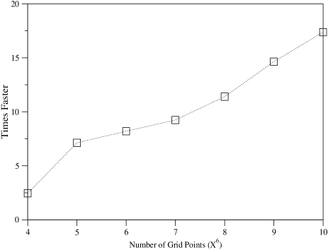
Figure 4: Efficiency of our modified Stone method when compared to the gmres routine of Matlab that handles sparse matrices. When we increase the number of grid points our method becomes more efficient. To handle the $9^{6}$ and $10^{6}$ grid in our computer, we lower the value of the restarting parameter of the GMRES routine to the maximum possible value that avoids computer memory problems.

where $\dot{\bf v}=-\nabla\Phi$, $\Phi=1/\sqrt{x^{2}+y^{2}+z^{2}+1^{2}}$, and $\beta$ is a constant. The form of Eq. (21) is similar to the equation found when Rosenbluth potentials ros:mac are used in a gravitational potential $\Phi$. Note that the collision term has mixed velocity derivatives and that the resulting coefficient matrix from the discretization is non symmetric. We used central difference and a twenty-five point molecule to perform the discretization of Eq. (21), see also Table 1. Here, we find the solution of the above equation in a six dimensional ‘box’ of length 1.22 units. At the borders we used a Dirichlet boundary condition of the form $f=\exp(-x^{2}-y^{2}-z^{2})\exp(-v_{x}^{2}-v_{y}^{2}-v_{z}^{2})$.

Figure 5: Numerical solutions of the distribution function of Eq. (21). Top: surface distribution for the case with $v_{x}\approx 0.38$, $v_{y}\approx-0.5$, $v_{z}\approx-0.5$ and $z\approx 0.16$. Bottom: velocity distribution for the case with $x\approx-0.39$, $y\approx 0.06$, $z\approx-0.17$ and $v_{x}\approx 0.28$.

We first started with coarse grid of four points per variable that leads to a matrix of $4096^{2}$ elements (in this number we are not considering the border grid points given by the boundary condition) and $\beta=1$. We found for this case that our method spent approximately 0.2 seconds to find the solution (all the calculations were perform with a Pentium IV of 1.8 GHz, the Fortran code was compiled with the Linux free compiler). We stop the iteration when $\sum_{i=1}^{n}(\Delta_{i}^{t+1})<10^{-10}$. The gmres routine and the public GMRES code fra:gir spent approximately 0.35 and 3 seconds respectively to solve the system of equations with the same stop criteria, but it could be more if we choose wrong the restarting parameter. Here we are considering only the time spent to solve the coefficient matrix and not the time due to create the coefficient matrix and upload it into the code. In our code, we only upload 25 vectors of approximately $N_{node}$.

For a grid of five points per variable some code compilers can not allow the storage of the coefficient matrix because is too large $5^{12}$, approximately 244 millions of elements. This was the case of the public code because it can not managed sparse matrices. For this number of grid points the modified Stone method was almost 7 times faster than the gmres routine. In Fig. 4 we present the efficiency of our method compare to the gmres routine. Note that when we increase the number of grid points the efficiency also increases. For a grid of nine points per variable the gmres routine can not managed to find the solution in one iteration because we have computer storage problems. To handle this, we lower the restarting parameter to the maximum possible value that avoids this problem. For a grid of ten point per variable the number of elements in the coefficient matrix increases to $10^{12}$. Our code can managed this huge amount of data in a faster and efficient way. The time spent for this case was approximately 85 seconds. This should be the time spent for each time step in a non stationary problem, which is a great result considering the number of nodes in the grid and the precision attained with the stop criteria. The variation of $\alpha$ between the accepted limits $0<\alpha<1$ slightly alter the time spent in finding the solution. In Fig. 5, we present two graphs of the distribution function from the numerical solution of Eq. (21) for a grid of ten grid per variable. One is the surface distribution function on the plane $x-y$ and the other is the velocity distribution function on the plane $v_{y}-v_{z}$; they are plotted at different points of the grid. Note that these figures have not Maxwellian form because Eq. (21) is not in the collisional regime for the parameters considered in the collision term. This example was chosen only for didactic reasons.

Note that when we used central difference for discretization of Eq. (21), the only contribution to the main diagonal comes from the last right hand term, i.e. the term with $\beta$. For some values of $\beta<1$ our code diverge because our resulting coefficient matrix is not diagonal dominant. For the same value of $\beta$, the gmres routine converges. The break in convergence at these values of $\beta$ coincide with the appearance of negatives values on the distribution function solution found by gmres. We know that one of condition to attained a physical solution of the Fokker-Planck equation is that the distribution function has to be always positive. It is remarkable that for Eq. (21) our code diverge when physical solutions are not possible, this could be an indication that we are applying a wrong scheme for discretization or that we are not describing well the physical phenomena considered. As we said in the Introduction, other discretization scheme may be applied to avoid this problem. Thus, in our method the convergence is conditioned to the form of the functions present in (1) and (2), i.e. physical considerations; and to the difference scheme applied for discretization, i.e. numerical implementation. For a non stationary scheme the Crank-Nicolson decomposition in time is suggested because it has implicit character and it is usually more stable than other methods, but strictly speaking, the stability of the system has to be studied for each particular case considered.

V Domains with curved boundaries

The $LU$ code was tested in the previous section with a structure-orthogonal grid but this does not mean that it can not be applied to more general geometries. To handle a non square domain we proceed as follows. First we make a square structured grid with $N_{node}=n_{i}n_{j}n_{k}n_{l}n_{m}n_{n}$ nodes, then we label them according to the index $p$ defined in (4). Later, the nodes that laid outside the boundary regions are not considered for the calculations. Now, lets see this procedure in an example. For didactic purpose we used only the one dimensional case of the Fokker-Planck equation in which we have two variables $(x,v_{x})$. In Fig. 6 is depicted in the two dimensional plane $(x,v_{x})$ a domain region $\Omega$ with boundary $\Omega_{B}$. The domain $\Omega$ is filled with a square structured grid that leads three classes of grid points: the interior points in which the normal discretization procedure can be done; the boundary points in which special care have to be taken when Dirichlet, Neumann or mixed boundary conditions are applied; and the exterior points that have to be neglected for the calculation, see Fig. 6.

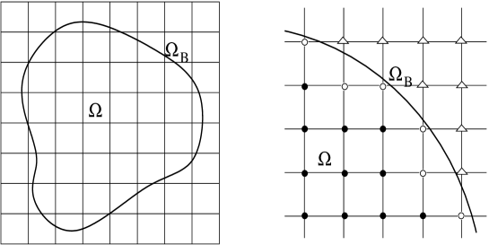
Figure 6: Application of the incomplete $LU$ decomposition to a general domain $\Omega$ with curved boundaries $\Omega_{B}$. The square structured grid leads three classes of grid points: interior points (full circles), boundary points (empty circles) and exterior points (triangles).

Figure 7: Schematic representation of a five-point molecule for the finite difference approximation of the derivatives in the plane $(x,v_{x})$ for a boundary point. Below, we see different boundary situations that can occur in the numerical computation depending on the discretization grid and boundary S.

The incorporation of the Dirichlet boundary conditions using central differences for the boundary points of region $\Omega$ can be done using a Taylor expansion around the nearest nodes. For example, in Fig. 7, we take the nearest boundary points for point 1: the internal node (node 2) and the point at the boundary $\Omega_{B}$ (point $E$); and make two Taylor expansions around point 1. These expansions give us (our conventions are: partial derivative with respect to the coordinate $x$ denoted by ($,x$); $\Delta x$ is the discretization interval in the $x$ direction),

$$\Psi_{E}=\Psi_{1}+b\Delta x\Psi_{,x}+\frac{(b\Delta x)^{2}}{2!}\Psi_{,xx}+O[\Delta x^{3}],$$

$$\Psi_{2}=\Psi_{1}-\Delta x\Psi_{,x}+\frac{(\Delta x)^{2}}{2!}\Psi_{,xx}+O[\Delta x^{3}],$$ (22)

eliminating the second order derivative between these equations we can express the partial derivative at a boundary point as,

$$\Psi_{,x}=\frac{1}{\Delta x}\left[\frac{1}{b(1+b)}\Psi_{E}-\frac{b}{1+b}\Psi_{2}-\frac{1-b}{b}\Psi_{1}\right]+O[\Delta x^{2}].$$ (23)

When $b=1$ we recover the usual expression for the central derivative. The same procedure can be applied to the northern boundary, between node 3 and point $A$, and to the different types of boundary nodes in Fig. 7. Also, partial derivative of higher orders and mixed derivatives can be found in a similar way. Furthermore, it is also possible to implement Neumann boundary conditions in an irregular boundary using finite difference, see for instance for:was .

The exterior points of Fig. 6 are strictly necessary to maintain the ordering of the nodes in a domain with curved boundaries. This ordering is needed by the code to operate normally but they do not enter into the calculations. To implement this condition, we have to set the values of the elements $L^{p}_{[X]}$, $L^{p}_{P}$, $U^{p}_{[X]}$, $R^{p}$, $\Upsilon^{p}$ and $\Delta^{p}$ of the external grid point (each exterior point has a position $p$ from the one dimensional storage index) equal to zero.

An application of the $LU$ method in a two dimensional Fokker-Planck equation ($x,y,v_{x},v_{y}$) with curved boundaries, as well as the incomplete $LU$ decomposition for this case can be seen in uje:let . Here, the distribution function of a stationary gravitational thin disk is calculated. Note that in order to obtain the elements of the $LU$ decomposition for the two dimensional case, we have to start the calculations from the beginning, i.e. we can not used the elements found in the three dimensional case.

VI Concluding Remarks

We have developed a variation of the incomplete $LU$ decomposition proposed by Stone that solves the three dimensional linear Fokker-Planck equation. The method presented can manage the large set of linear equations that appears from the discretization procedure. The convergence of the iterative process is done in a fast and effective way. Also, this method can be easily adapted to support irregular boundaries with Dirichlet, Neumann or mixed boundary conditions and can be used to follow the evolution of a distribution function for non stationary equations. In this case a Crank-Nicolson discretization in time is recommended because it has implicit character and is more stable than other methods, but strictly speaking, the stability of the system has to be studied in each particular case considered. The good properties that our method shares and the lack of methods that handle the large amount of data (given by the Fokker-Planck equation with six independent variables) make the method presented in this article worthy and advantageous. In general, the algorithm presented in the article can solve the system of equations that arises from the discretization of the equation (1) or similar equations (with or without the mixed derivatives), but we have to keep in mind that its convergence is conditioned to the form of the functions $\dot{\bf v}$, $A({\bf x,v})$, $B({\bf x,v})$, $C({\bf x,v})$, $D({\bf x,v})$ and $E_{ij}({\bf x,v})$ that appear in the collision term (2).

Appendix A Elements of $M=LU$ at node $p$

In this section we present how the elements of the matrix $M$ are related to the elements of the upper $U$ and lower $L$ matrices.

$$M^{p}_{DD3}=L^{p}_{DD3},$$

$$M^{p}_{DD3|N}=L^{p}_{DD3}U^{p-(n_{ijklm}+n_{ijkl})}_{N},$$

$$M^{p}_{DD3|E}=L^{p}_{DD3}U^{p-(n_{ijklm}+n_{ijkl})}_{E},$$

$$M^{p}_{DD3|T}=L^{p}_{DD3}U^{p-(n_{ijklm}+n_{ijkl})}_{T},$$

$$M^{p}_{DD3|U1}=L^{p}_{DD3}U^{p-(n_{ijklm}+n_{ijkl})}_{U1},$$

$$M^{p}_{DB3}=L^{p}_{DB3}+L^{p}_{DD3}U^{p-(n_{ijklm}+n_{ijkl})}_{UB2},$$

$$M^{p}_{DB3|N}=L^{p}_{DB3}U^{p-(n_{ijklm}+n_{ijk})}_{N},$$

$$M^{p}_{DB3|E}=L^{p}_{DB3}U^{p-(n_{ijklm}+n_{ijk})}_{E},$$

$$M^{p}_{DB3|T}=L^{p}_{DB3}U^{p-(n_{ijklm}+n_{ijk})}_{T},$$

$$M^{p}_{D3}=L^{p}_{D3}+L^{p}_{DB3}U^{p-(n_{ijklm}+n_{ijk})}_{U1}+L^{p}_{DD3}U^{p-(n_{ijklm}+n_{ijkl})}_{U2},$$

$$M^{p}_{D3|N}=L^{p}_{D3}U^{p-n_{ijklm}}_{N},$$

$$M^{p}_{D3|E}=L^{p}_{D3}U^{p-n_{ijklm}}_{E},$$

$$M^{p}_{D3|T}=L^{p}_{D3}U^{p-n_{ijklm}}_{T},$$

$$M^{p}_{DT3}=L^{p}_{DT3}+L^{p}_{D3}U^{p-n_{ijklm}}_{U1}+L^{p}_{DD3}U^{p-(n_{ijklm}+n_{ijkl})}_{UT2},$$

$$M^{p}_{DT3|N}=L^{p}_{DT3}U^{p-(n_{ijklm}-n_{ijk})}_{N},$$

$$M^{p}_{DT3|E}=L^{p}_{DT3}U^{p-(n_{ijklm}-n_{ijk})}_{E},$$

$$M^{p}_{DT3|T}=L^{p}_{DT3}U^{p-(n_{ijklm}-n_{ijk})}_{T},$$

$$M^{p}_{DT3|U1}=L^{p}_{DT3}U^{p-(n_{ijklm}-n_{ijk})}_{U1},$$

$$M^{p}_{DB3|UB2}=L^{p}_{DB3}U^{p-(n_{ijklm}+n_{ijk})}_{UB2},$$

$$M^{p}_{D3|UB2}=L^{p}_{D3}U^{p-n_{ijklm}}_{UB2}+L^{p}_{DB3}U^{p-(n_{ijklm}+n_{ijk})}_{U2},$$

$$M^{p}_{DU3}=L^{p}_{DU3}+L^{p}_{DT3}U^{p-(n_{ijklm}-n_{ijk})}_{UB2}+L^{p}_{D3}U^{p-n_{ijklm}}_{U2}+L^{p}_{DB3}U^{p-(n_{ijklm}+n_{ijk})}_{UT2},$$

$$M^{p}_{DU3|N}=L^{p}_{DU3}U^{p-(n_{ijklm}-n_{ijkl})}_{N},$$

$$M^{p}_{DU3|E}=L^{p}_{DU3}U^{p-(n_{ijklm}-n_{ijkl})}_{E},$$

$$M^{p}_{DU3|T}=L^{p}_{DU3}U^{p-(n_{ijklm}-n_{ijkl})}_{T},$$

$$M^{p}_{DU3|U1}=L^{p}_{DU3}U^{p-(n_{ijklm}-n_{ijkl})}_{U1}+L^{p}_{DT3}U^{p-(n_{ijklm}-n_{ijk})}_{U2}+L^{p}_{D3}U^{p-n_{ijklm}}_{UT2},$$

$$M^{p}_{DT3|UT2}=L^{p}_{DT3}U^{p-(n_{ijklm}-n_{ijk})}_{UT2},$$

$$M^{p}_{DU3|UB2}=L^{p}_{DU3}U^{p-(n_{ijklm}-n_{ijkl})}_{UB2},$$

$$M^{p}_{DU3|U2}=L^{p}_{DU3}U^{p-(n_{ijklm}-n_{ijkl})}_{U2},$$

$$M^{p}_{DU3|UT2}=L^{p}_{DU3}U^{p-(n_{ijklm}-n_{ijkl})}_{UT2},$$

$$M^{p}_{DD3|UD3}=L^{p}_{DD3}U^{p-(n_{ijklm}+n_{ijkl})}_{UD3},$$

$$M^{p}_{DB2}=L^{p}_{DB2}+L^{p}_{DB3}U^{p-(n_{ijklm}+n_{ijk})}_{UD3}+L^{p}_{DD3}U^{p-(n_{ijklm}+n_{ijkl})}_{UB3},$$

$$M^{p}_{DB2|N}=L^{p}_{DB2}U^{p-(n_{ijkl}+n_{ijk})}_{N},$$

$$M^{p}_{DB2|E}=L^{p}_{DB2}U^{p-(n_{ijkl}+n_{ijk})}_{E},$$

$$M^{p}_{DB2|T}=L^{p}_{DB2}U^{p-(n_{ijkl}+n_{ijk})}_{T},$$

$$M^{p}_{D2}=L^{p}_{D2}+L^{p}_{DB2}U^{p-(n_{ijkl}+n_{ijk})}_{U1}+L^{p}_{D3}U^{p-n_{ijklm}}_{UD3}+L^{p}_{DD3}U^{p-(n_{ijklm}+n_{ijkl})}_{U3},$$

$$M^{p}_{D2|N}=L^{p}_{D2}U^{p-n_{ijkl}}_{N},$$

$$M^{p}_{D2|E}=L^{p}_{D2}U^{p-n_{ijkl}}_{E},$$

$$M^{p}_{D2|T}=L^{p}_{D2}U^{p-n_{ijkl}}_{T},$$

$$M^{p}_{DT2}=L^{p}_{DT2}+L^{p}_{D2}U^{p-n_{ijkl}}_{U1}+L^{p}_{DT3}U^{p-(n_{ijklm}-n_{ijk})}_{UD3}+L^{p}_{DD3}U^{p-(n_{ijklm}+n_{ijkl})}_{UT3},$$

$$M^{p}_{DT2|N}=L^{p}_{DT2}U^{p-(n_{ijkl}-n_{ijk})}_{N},$$

$$M^{p}_{DT2|E}=L^{p}_{DT2}U^{p-(n_{ijkl}-n_{ijk})}_{E},$$

$$M^{p}_{DT2|T}=L^{p}_{DT2}U^{p-(n_{ijkl}-n_{ijk})}_{T},$$

$$M^{p}_{DT2|U1}=L^{p}_{DT2}U^{p-(n_{ijkl}-n_{ijk})}_{U1},$$

$$M^{p}_{DB2|UB2}=L^{p}_{DB2}U^{p-(n_{ijkl}+n_{ijk})}_{UB2}+L^{p}_{DB3}U^{p-(n_{ijklm}+n_{ijk})}_{UB3},$$

$$M^{p}_{D1}=L^{p}_{D1}+L^{p}_{D2}U^{p-n_{ijkl}}_{UB2}+L^{p}_{DB2}U^{p-(n_{ijkl}+n_{ijk})}_{U2}+L^{p}_{D3}U^{p-n_{ijklm}}_{UB3}+L^{p}_{DB3}U^{p-(n_{ijklm}+n_{ijk})}_{U3},$$

$$M^{p}_{D1|N}=L^{p}_{D1}U^{p-n_{ijk}}_{N},$$

$$M^{p}_{D1|E}=L^{p}_{D1}U^{p-n_{ijk}}_{E},$$

$$M^{p}_{D1|T}=L^{p}_{D1}U^{p-n_{ijk}}_{T},$$

$$M^{p}_{B}=L^{p}_{B},$$

$$M^{p}_{B|N}=L^{p}_{B}U^{p-n_{ij}}_{N},$$

$$M^{p}_{B|E}=L^{p}_{B}U^{p-n_{ij}}_{E},$$

$$M^{p}_{W}=L^{p}_{W},$$

$$M^{p}_{W|N}=L^{p}_{W}U^{p-n_{j}}_{N},$$

$$M^{p}_{S}=L^{p}_{S},$$

$$M^{p}_{P}=L^{p}_{P}+L^{p}_{S}U^{p-1}_{N}+L^{p}_{W}U^{p-n_{j}}_{E}+L^{p}_{B}U^{p-n_{ij}}_{T}+L^{p}_{D1}U^{p-n_{ijk}}_{U1}+L^{p}_{DT2}U^{p-(n_{ijkl}-n_{ijk})}_{UB2}+L^{p}_{D2}U^{p-n_{ijkl}}_{U2}$$

$$\hskip 28.45274pt+L^{p}_{DB2}U^{p-(n_{ijkl}+n_{ijk})}_{UT2}+L^{p}_{DU3}U^{p-(n_{ijklm}-n_{ijkl})}_{UD3}+L^{p}_{DT3}U^{p-(n_{ijklm}-n_{ijk})}_{UB3}+L^{p}_{D3}U^{p-n_{ijklm}}_{U3}$$

$$\hskip 28.45274pt+L^{p}_{DB3}U^{p-(n_{ijklm}+n_{ijk})}_{UT3}+L^{p}_{DD3}U^{p-(n_{ijklm}+n_{ijkl})}_{UU3},$$

$$M^{p}_{N}=L^{p}_{P}U^{p}_{N},$$

$$M^{p}_{S|E}=L^{p}_{S}U^{p-1}_{E},$$

$$M^{p}_{E}=L^{p}_{P}U^{p}_{E},$$

$$M^{p}_{W|T}=L^{p}_{W}U^{p-n_{j}}_{T},$$

$$M^{p}_{S|T}=L^{p}_{S}U^{p-1}_{T},$$

$$M^{p}_{T}=L^{p}_{P}U^{p}_{T},$$

$$M^{p}_{B|U1}=L^{p}_{B}U^{p-n_{ij}}_{U1},$$

$$M^{p}_{W|U1}=L^{p}_{W}U^{p-n_{j}}_{U1},$$

$$M^{p}_{S|U1}=L^{p}_{S}U^{p-1}_{U1},$$

$$M^{p}_{U1}=L^{p}_{P}U^{p}_{U1}+L^{p}_{DT2}U^{p-(n_{ijkl}-n_{ijk})}_{U2}+L^{p}_{D2}U^{p-n_{ijkl}}_{UT2}+L^{p}_{DT3}U^{p-(n_{ijklm}-n_{ijk})}_{U3}+L^{p}_{D3}U^{p-n_{ijklm}}_{UT3},$$

$$M^{p}_{DT2|UT2}=L^{p}_{DT2}U^{p-(n_{ijkl}-n_{ijk})}_{UT2}+L^{p}_{DT3}U^{p-(n_{ijklm}-n_{ijk})}_{UT3},$$

$$M^{p}_{D1|UB2}=L^{p}_{D1}U^{p-n_{ijk}}_{UB2},$$

$$M^{p}_{B|UB2}=L^{p}_{B}U^{p-n_{ij}}_{UB2},$$

$$M^{p}_{W|UB2}=L^{p}_{W}U^{p-n_{j}}_{UB2},$$

$$M^{p}_{S|UB2}=L^{p}_{S}U^{p-1}_{UB2},$$

$$M^{p}_{UB2}=L^{p}_{P}U^{p}_{UB2}+L^{p}_{D1}U^{p-n_{ijk}}_{U2}+L^{p}_{DU3}U^{p-(n_{ijklm}-n_{ijkl})}_{UB3}+L^{p}_{DB3}U^{p-(n_{ijklm}+n_{ijk})}_{UU3},$$

$$M^{p}_{B|U2}=L^{p}_{B}U^{p-n_{ij}}_{U2},$$

$$M^{p}_{W|U2}=L^{p}_{W}U^{p-n_{j}}_{U2},$$

$$M^{p}_{S|U2}=L^{p}_{S}U^{p-1}_{U2},$$

$$M^{p}_{U2}=L^{p}_{P}U^{p}_{U2}+L^{p}_{D1}U^{p-n_{ijk}}_{UT2}+L^{p}_{DU3}U^{p-(n_{ijklm}-n_{ijkl})}_{U3}+L^{p}_{D3}U^{p-n_{ijklm}}_{UU3},$$

$$M^{p}_{B|UT2}=L^{p}_{B}U^{p-n_{ij}}_{UT2},$$

$$M^{p}_{W|UT2}=L^{p}_{W}U^{p-n_{j}}_{UT2},$$

$$M^{p}_{S|UT2}=L^{p}_{S}U^{p-1}_{UT2},$$

$$M^{p}_{UT2}=L^{p}_{P}U^{p}_{UT2}+L^{p}_{DU3}U^{p-(n_{ijklm}-n_{ijkl})}_{UT3}+L^{p}_{DT3}U^{p-(n_{ijklm}-n_{ijk})}_{UU3},$$

$$M^{p}_{DU3|UU3}=L^{p}_{DU3}U^{p-(n_{ijklm}-n_{ijkl})}_{UU3},$$

$$M^{p}_{DB2|UD3}=L^{p}_{DB2}U^{p-(n_{ijkl}+n_{ijk})}_{UD3},$$

$$M^{p}_{D2|UD3}=L^{p}_{D2}U^{p-n_{ijkl}}_{UD3},$$

$$M^{p}_{DT2|UD3}=L^{p}_{DT2}U^{p-(n_{ijkl}-n_{ijk})}_{UD3},$$

$$M^{p}_{DB2|UB3}=L^{p}_{DB2}U^{p-(n_{ijkl}+n_{ijk})}_{UB3},$$

$$M^{p}_{D1|UD3}=L^{p}_{D1}U^{p-n_{ijk}}_{UD3}+L^{p}_{D2}U^{p-n_{ijkl}}_{UB3}+L^{p}_{DB2}U^{p-(n_{ijkl}+n_{ijk})}_{U3},$$

$$M^{p}_{B|UD3}=L^{p}_{B}U^{p-n_{ij}}_{UD3},$$

$$M^{p}_{W|UD3}=L^{p}_{W}U^{p-n_{j}}_{UD3},$$

$$M^{p}_{S|UD3}=L^{p}_{S}U^{p-1}_{UD3},$$

$$M^{p}_{UD3}=L^{p}_{P}U^{p}_{UD3}+L^{p}_{DT2}U^{p-(n_{ijkl}-n_{ijk})}_{UB3}+L^{p}_{D2}U^{p-n_{ijkl}}_{U3}+L^{p}_{DB2}U^{p-(n_{ijkl}+n_{ijk})}_{UT3},$$

$$M^{p}_{DT2|U3}=L^{p}_{DT2}U^{p-(n_{ijkl}-n_{ijk})}_{U3}+L^{p}_{D2}U^{p-n_{ijkl}}_{UT3},$$

$$M^{p}_{DT2|UT3}=L^{p}_{DT2}U^{p-(n_{ijkl}-n_{ijk})}_{UT3},$$

$$M^{p}_{D1|UB3}=L^{p}_{D1}U^{p-n_{ijk}}_{UB3},$$

$$M^{p}_{B|UB3}=L^{p}_{B}U^{p-n_{ij}}_{UB3},$$

$$M^{p}_{W|UB3}=L^{p}_{W}U^{p-n_{j}}_{UB3},$$

$$M^{p}_{S|UB3}=L^{p}_{S}U^{p-1}_{UB3},$$

$$M^{p}_{UB3}=L^{p}_{P}U^{p}_{UB3}+L^{p}_{D1}U^{p-n_{ijk}}_{U3}+L^{p}_{DB2}U^{p-(n_{ijkl}+n_{ijk})}_{UU3},$$

$$M^{p}_{B|U3}=L^{p}_{B}U^{p-n_{ij}}_{U3},$$

$$M^{p}_{W|U3}=L^{p}_{W}U^{p-n_{j}}_{U3},$$

$$M^{p}_{S|U3}=L^{p}_{S}U^{p-1}_{U3},$$

$$M^{p}_{U3}=L^{p}_{P}U^{p}_{U3}+L^{p}_{D1}U^{p-n_{ijk}}_{UT3}+L^{p}_{D2}U^{p-n_{ijkl}}_{UU3},$$

$$M^{p}_{B|UT3}=L^{p}_{B}U^{p-n_{ij}}_{UT3},$$

$$M^{p}_{W|UT3}=L^{p}_{W}U^{p-n_{j}}_{UT3},$$

$$M^{p}_{S|UT3}=L^{p}_{S}U^{p-1}_{UT3},$$

$$M^{p}_{UT3}=L^{p}_{P}U^{p}_{UT3}+L^{p}_{DT2}U^{p-(n_{ijkl}-n_{ijk})}_{UU3},$$

$$M^{p}_{D1|UU3}=L^{p}_{D1}U^{p-n_{ijk}}_{UU3},$$

$$M^{p}_{B|UU3}=L^{p}_{B}U^{p-n_{ij}}_{UU3},$$

$$M^{p}_{W|UU3}=L^{p}_{W}U^{p-n_{j}}_{UU3},$$

$$M^{p}_{S|UU3}=L^{p}_{S}U^{p-1}_{UU3},$$

$$M^{p}_{UU3}=L^{p}_{P}U^{p}_{UU3}.$$ (24)

Appendix B Explicit Form of Eq. (9)

In this section we present the explicit form of $O\Psi\approx 0$ for each grid node.

$$O_{DD3}\Psi_{DD3}+O_{DB3}\Psi_{DB3}+O_{D3}\Psi_{D3}+O_{DT3}\Psi_{DT3}+O_{DU3}\Psi_{DU3}+O_{DB2}\Psi_{DB2}+O_{D2}\Psi_{D2}+O_{DT2}\Psi_{DT2}$$

$$+O_{D1}\Psi_{D1}+O_{B}\Psi_{B}+O_{W}\Psi_{W}+O_{S}\Psi_{S}+O_{P}\Psi_{P}+O_{N}\Psi_{N}+O_{E}\Psi_{E}+O_{T}\Psi_{T}+O_{U1}\Psi_{U1}+O_{UB2}\Psi_{UB2}$$

$$+O_{U2}\Psi_{U2}+O_{UT2}\Psi_{UT2}+O_{UD3}\Psi_{UD3}+O_{UB3}\Psi_{UB3}+O_{U3}\Psi_{U3}+O_{UT3}\Psi_{UT3}+O_{UU3}\Psi_{UU3}+M_{DD3|N}\Psi_{DD3|N}$$

$$+M_{DD3|E}\Psi_{DD3|E}+M_{DD3|T}\Psi_{DD3|T}+M_{DD3|U1}\Psi_{DD3|U1}+M_{DB3|N}\Psi_{DB3|N}+M_{DB3|E}\Psi_{DB3|E}$$

$$+M_{DB3|T}\Psi_{DB3|T}+M_{D3|N}\Psi_{D3|N}+M_{D3|E}\Psi_{D3|E}+M_{D3|T}\Psi_{D3|T}+M_{DT3|N}\Psi_{DT3|N}+M_{DT3|E}\Psi_{DT3|E}$$

$$+M_{DT3|T}\Psi_{DT3|T}+M_{DT3|U1}\Psi_{DT3|U1}+M_{DB3|UB2}\Psi_{DB3|UB2}+M_{DB3|U2}\Psi_{DB3|U2}+M_{D3|UB2}\Psi_{D3|UB2}$$

$$+M_{DU3|N}\Psi_{DU3|N}+M_{DU3|E}\Psi_{DU3|E}+M_{DU3|T}\Psi_{DU3|T}+M_{D3|UT2}\Psi_{D3|UT2}+M_{DT3|U2}\Psi_{DT3|U2}$$

$$+M_{DU3|U1}\Psi_{DU3|U1}+M_{DT3|UT2}\Psi_{DT3|UT2}+M_{DU3|UB2}\Psi_{DU3|UB2}+M_{DU3|U2}\Psi_{DU3|U2}+M_{DU3|UT2}\Psi_{DU3|UT2}$$

$$+M_{DD3|UD3}\Psi_{DD3|UD3}+M_{DB2|N}\Psi_{DB2|N}+M_{DB2|E}\Psi_{DB2|E}+M_{DB2|T}\Psi_{DB2|T}+M_{D2|N}\Psi_{D2|N}+M_{D2|E}\Psi_{D2|E}$$

$$+M_{D2|T}\Psi_{D2|T}+M_{DT2|N}\Psi_{DT2|N}+M_{DT2|E}\Psi_{DT2|E}+M_{DT2|T}\Psi_{DT2|T}+M_{DT2|U1}\Psi_{DT2|U1}$$

$$+M_{DB3|UB3}\Psi_{DB3|UB3}+M_{DB2|UB2}\Psi_{DB2|UB2}+M_{D1|N}\Psi_{D1|N}+M_{D1|E}\Psi_{D1|E}+M_{D1|T}\Psi_{D1|T}+M_{B|N}\Psi_{B|N}$$

$$+M_{B|E}\Psi_{B|E}+M_{W|N}\Psi_{W|N}+M_{S|E}\Psi_{S|E}+M_{W|T}\Psi_{W|T}+M_{S|T}\Psi_{S|T}+M_{B|U1}\Psi_{B|U1}+M_{W|U1}\Psi_{W|U1}$$

$$+M_{S|U1}\Psi_{S|U1}+M_{DT2|UT2}\Psi_{DT2|UT2}+M_{DT3|UT3}\Psi_{DT3|UT3}+M_{D1|UB2}\Psi_{D1|UB2}+M_{B|UB2}\Psi_{B|UB2}$$

$$+M_{W|UB2}\Psi_{W|UB2}+M_{S|UB2}\Psi_{S|UB2}+M_{B|U2}\Psi_{B|U2}+M_{W|U2}\Psi_{W|U2}+M_{S|U2}\Psi_{S|U2}+M_{B|UT2}\Psi_{B|UT2}$$

$$+M_{W|UT2}\Psi_{W|UT2}+M_{S|UT2}\Psi_{S|UT2}+M_{DU3|UU3}\Psi_{DU3|UU3}+M_{DB2|UD3}\Psi_{DB2|UD3}+M_{D2|UD3}\Psi_{D2|UD3}$$

$$+M_{DT2|UD3}\Psi_{DT2|UD3}+M_{DB2|UB3}\Psi_{DB2|UB3}+M_{D1|UD3}\Psi_{D1|UD3}+M_{D2|UB3}\Psi_{D2|UB3}+M_{DB2|U3}\Psi_{DB2|U3}$$

$$+M_{B|UD3}\Psi_{B|UD3}+M_{W|UD3}\Psi_{W|UD3}+M_{S|UD3}\Psi_{S|UD3}+M_{DT2|U3}\Psi_{DT2|U3}+M_{D2|UT3}\Psi_{D2|UT3}$$

$$+M_{DT2|UT3}\Psi_{DT2|UT3}+M_{D1|UB3}\Psi_{D1|UB3}+M_{B|UB3}\Psi_{B|UB3}+M_{W|UB3}\Psi_{W|UB3}+M_{S|UB3}\Psi_{S|UB3}$$

$$+M_{B|U3}\Psi_{B|U3}+M_{W|U3}\Psi_{W|U3}+M_{S|U3}\Psi_{S|U3}+M_{B|UT3}\Psi_{B|UT3}+M_{W|UT3}\Psi_{W|UT3}+M_{S|UT3}\Psi_{S|UT3}$$

$$+M_{D1|UU3}\Psi_{D1|UU3}+M_{B|UU3}\Psi_{B|UU3}+M_{W|UU3}\Psi_{W|UU3}+M_{S|UU3}\Psi_{S|UU3}\approx 0.$$ (25)

Appendix C $O$ as a Linear Combination of $M$

In this section we present the elements of the matrix $O$ as a linear combination of the elements of matrix $M$ using the relations (10).

$$O_{DD3}=-\alpha(M_{DD3|N}+M_{DD3|E}+M_{DD3|T}+M_{DD3|U1}+M_{DD3|UD3}),$$

$$O_{DB3}=-\alpha(M_{DB3|N}+M_{DB3|E}+M_{DB3|T}+M_{DB3|UB2}+M_{DB3|U2}+M_{DB3|UB3}),$$

$$O_{D3}=-\alpha(M_{D3|N}+M_{D3|E}+M_{D3|T}+M_{D3|UB2}+M_{D3|UT2}),$$

$$O_{DT3}=-\alpha(M_{DT3|N}+M_{DT3|E}+M_{DT3|T}+M_{DT3|U1}+M_{DT3|U2}+M_{DT3|UT2}+M_{DT3|UT3}),$$

$$O_{DU3}=-\alpha(M_{DU3|N}+M_{DU3|E}+M_{DU3|T}+M_{DU3|U1}+M_{DU3|UB2}+M_{DU3|U2}+M_{DU3|UT2}+M_{DU3|UU3}),$$

$$O_{DB2}=-\alpha(M_{DB2|N}+M_{DB2|E}+M_{DB2|T}+M_{DB2|UB2}+M_{DB2|UD3}+M_{DB2|UB3}+M_{DB2|U3}),$$

$$O_{D2}=-\alpha(M_{D2|N}+M_{D2|E}+M_{D2|T}+M_{D2|UD3}+M_{D2|UB3}+M_{D2|UT3}),$$

$$O_{DT2}=-\alpha(M_{DT2|N}+M_{DT2|E}+M_{DT2|T}+M_{DT2|U1}+M_{DT2|UT2}+M_{DT2|UD3}+M_{DT2|U3}+M_{DT2|UT3}),$$

$$O_{D1}=-\alpha(M_{D1|N}+M_{D1|E}+M_{D1|T}+M_{D1|UB2}+M_{D1|UD3}+M_{D1|UB3}+M_{D1|UU3}),$$

$$O_{B}=-\alpha(M_{B|N}+M_{B|E}+M_{B|U1}+M_{B|UB2}+M_{B|U2}+M_{B|UT2}+M_{B|UD3}+M_{B|UB3}+M_{B|U3}+M_{B|UT3}$$

$$\hskip 28.45274pt+M_{B|UU3}),$$

$$O_{W}=-\alpha(M_{W|N}+M_{W|T}+M_{W|U1}+M_{W|UB2}+M_{W|U2}+M_{W|UT2}+M_{W|UD3}+M_{W|UB3}+M_{W|U3}+M_{W|UT3}$$

$$\hskip 28.45274pt+M_{W|UU3}),$$

$$O_{S}=-\alpha(M_{S|E}+M_{S|T}+M_{S|U1}+M_{S|UB2}+M_{S|U2}+M_{S|UT2}+M_{S|UD3}+M_{S|UB3}+M_{S|U3}+M_{S|UT3}$$

$$\hskip 28.45274pt+M_{S|UU3}),$$

$$O_{P}=\alpha(M_{DD3|N}+M_{DD3|E}+M_{DD3|T}+M_{DD3|U1}+M_{DB3|N}+M_{DB3|E}+M_{DB3|T}+M_{D3|N}+M_{D3|E}+M_{D3|T}$$

$$\hskip 28.45274pt+M_{DT3|N}+M_{DT3|E}+M_{DT3|T}+M_{DT3|U1}+M_{DB3|UB2}+M_{DB3|U2}+M_{D3|UB2}+M_{DU3|N}+M_{DU3|E}$$

$$\hskip 28.45274pt+M_{DU3|T}+M_{D3|UT2}+M_{DT3|U2}+M_{DU3|U1}+M_{DT3|UT2}+M_{DU3|UB2}+M_{DU3|U2}+M_{DU3|UT2}$$

$$\hskip 28.45274pt+M_{DD3|UD3}+M_{DB2|N}+M_{DB2|E}+M_{DB2|T}+M_{D2|N}+M_{D2|E}+M_{D2|T}+M_{DT2|N}+M_{DT2|E}+M_{DT2|T}$$

$$\hskip 28.45274pt+M_{DT2|U1}+M_{DB3|UB3}+M_{DB2|UB2}+M_{D1|N}+M_{D1|E}+M_{D1|T}+M_{B|N}+M_{B|E}+M_{W|N}+M_{S|E}$$

$$\hskip 28.45274pt+M_{W|T}+M_{S|T}+M_{B|U1}+M_{W|U1}+M_{S|U1}+M_{DT2|UT2}+M_{DT3|UT3}+M_{D1|UB2}+M_{B|UB2}+M_{W|UB2}$$

$$\hskip 28.45274pt+M_{S|UB2}+M_{B|U2}+M_{W|U2}+M_{S|U2}+M_{B|UT2}+M_{W|UT2}+M_{S|UT2}+M_{DU3|UU3}+M_{DB2|UD3}$$

$$\hskip 28.45274pt+M_{D2|UD3}+M_{DT2|UD3}+M_{DB2|UB3}+M_{D1|UD3}+M_{D2|UB3}+M_{DB2|U3}+M_{B|UD3}+M_{W|UD3}+M_{S|UD3}$$

$$\hskip 28.45274pt+M_{DT2|U3}+M_{D2|UT3}+M_{DT2|UT3}+M_{D1|UB3}+M_{B|UB3}+M_{W|UB3}+M_{S|UB3}+M_{B|U3}+M_{W|U3}$$

$$\hskip 28.45274pt+M_{S|U3}+M_{B|UT3}+M_{W|UT3}+M_{S|UT3}+M_{D1|UU3}+M_{B|UU3}+M_{W|UU3}+M_{S|UU3}),$$

$$O_{N}=-\alpha(M_{DD3|N}+M_{DB3|N}+M_{D3|N}+M_{DT3|N}+M_{DU3|N}+M_{DB2|N}+M_{D2|N}+M_{DT2|N}+M_{D1|N}+M_{B|N}$$

$$\hskip 28.45274pt+M_{W|N}),$$

$$O_{E}=-\alpha(M_{DD3|E}+M_{DB3|E}+M_{D3|E}+M_{DT3|E}+M_{DU3|E}+M_{DB2|E}+M_{D2|E}+M_{DT2|E}+M_{D1|E}+M_{B|E}$$

$$\hskip 28.45274pt+M_{S|E}),$$

$$O_{T}=-\alpha(M_{DD3|T}+M_{DB3|T}+M_{D3|T}+M_{DT3|T}+M_{DU3|T}+M_{DB2|T}+M_{D2|T}+M_{DT2|T}+M_{D1|T}+M_{W|T}$$

$$\hskip 28.45274pt+M_{S|T}),$$

$$O_{U1}=-\alpha(M_{DD3|U1}+M_{DT3|U1}+M_{DU3|U1}+M_{DT2|U1}+M_{B|U1}+M_{W|U1}+M_{S|U1}),$$

$$O_{UB2}=-\alpha(M_{DB3|UB2}+M_{D3|UB2}+M_{DU3|UB2}+M_{DB2|UB2}+M_{D1|UB2}+M_{B|UB2}+M_{W|UB2}+M_{S|UB2}),$$

$$O_{U2}=-\alpha(M_{DB3|U2}+M_{DT3|U2}+M_{DU3|U2}+M_{B|U2}+M_{W|U2}+M_{S|U2}),$$

$$O_{UT2}=-\alpha(M_{D3|UT2}+M_{DT3|UT2}+M_{DU3|UT2}+M_{DT2|UT2}+M_{B|UT2}+M_{W|UT2}+M_{S|UT2}),$$

$$O_{UD3}=-\alpha(M_{DD3|UD3}+M_{DB2|UD3}+M_{D2|UD3}+M_{DT2|UD3}+M_{D1|UD3}+M_{B|UD3}+M_{W|UD3}+M_{S|UD3}),$$

$$O_{UB3}=-\alpha(M_{DB3|UB3}+M_{DB2|UB3}+M_{D2|UB3}+M_{D1|UB3}+M_{B|UB3}+M_{W|UB3}+M_{S|UB3}),$$

$$O_{U3}=-\alpha(M_{DB2|U3}+M_{DT2|U3}+M_{B|U3}+M_{W|U3}+M_{S|U3}),$$

$$O_{UT3}=-\alpha(M_{DT3|UT3}+M_{D2|UT3}+M_{DT2|UT3}+M_{B|UT3}+M_{W|UT3}+M_{S|UT3}),$$

$$O_{UU3}=-\alpha(M_{DU3|UU3}+M_{D1|UU3}+M_{B|UU3}+M_{W|UU3}+M_{S|UU3}).$$ (26)

Appendix D Explicit form of the functions $C_{[X]}$ and $K_{[X]}$

In this section we show the functions $C_{[X]}$ and $K_{[X]}$ that appear in the final expression (11) of the $LU$ decomposition.

$$C_{DB3}=L_{DD3}^{p}U_{UB2}^{p-(n_{ijklm}+n_{ijkl})},$$

$$C_{D3}=L_{DD3}^{p}U_{U2}^{p-(n_{ijklm}+n_{ijkl})}+L_{DB3}^{p}U_{U1}^{p-(n_{ijklm}+n_{ijk})},$$

$$C_{DT3}=L_{DD3}^{p}U_{UT2}^{p-(n_{ijklm}+n_{ijkl})}+L_{D3}^{p}U_{U1}^{p-n_{ijklm}},$$

$$C_{DU3}=L_{DB3}^{p}U_{UT2}^{p-(n_{ijklm}+n_{ijk})}+L_{D3}^{p}U_{U2}^{p-n_{ijklm}}+L_{DT3}^{p}U_{UB2}^{p-(n_{ijklm}-n_{ijk})},$$

$$C_{DB2}=L_{DD3}^{p}U_{UB3}^{p-(n_{ijklm}+n_{ijkl})}+L_{DB3}^{p}U_{UD3}^{p-(n_{ijklm}+n_{ijk})},$$

$$C_{D2}=L_{DD3}^{p}U_{U3}^{p-(n_{ijklm}+n_{ijkl})}+L_{D3}^{p}U_{UD3}^{p-n_{ijklm}}+L_{DB2}^{p}U_{U1}^{p-(n_{ijkl}+n_{ijk})},$$

$$C_{DT2}=L_{DD3}^{p}U_{UT3}^{p-(n_{ijklm}+n_{ijkl})}+L_{DT3}^{p}U_{UD3}^{p-(n_{ijklm}-n_{ijk})}+L_{D2}^{p}U_{U1}^{p-n_{ijkl}},$$

$$C_{D1}=L_{DB3}^{p}U_{U3}^{p-(n_{ijklm}+n_{ijk})}+L_{D3}^{p}U_{UB3}^{p-n_{ijklm}}+L_{DB2}^{p}U_{U2}^{p-(n_{ijkl}+n_{ijk})}+L_{D2}^{p}U_{UB2}^{p-n_{ijkl}},$$

$$C_{U1}=L_{DT2}^{p}U_{U2}^{p-(n_{ijkl}-n_{ijk})}+L_{D2}^{p}U_{UT2}^{p-n_{ijkl}}+L_{DT3}^{p}U_{U3}^{p-(n_{ijklm}-n_{ijk})}+L_{D3}^{p}U_{UT3}^{p-n_{ijklm}},$$

$$C_{UB2}=L_{D1}^{p}U_{U2}^{p-n_{ijk}}+L_{DU3}^{p}U_{UB3}^{p-(n_{ijklm}-n_{ijkl})}+L_{DB3}^{p}U_{UU3}^{p-(n_{ijklm}+n_{ijk})},$$

$$C_{U2}=L_{D1}^{p}U_{UT2}^{p-n_{ijk}}+L^{p}_{DU3}U_{U3}^{p-(n_{ijklm}-n_{ijkl})}+L_{D3}^{p}U_{UU3}^{p-n_{ijklm}},$$

$$C_{UT2}=L_{DU3}^{p}U_{UT3}^{p-(n_{ijklm}-n_{ijkl})}+L_{DT3}^{p}U_{UU3}^{p-(n_{ijklm}-n_{ijk})},$$

$$C_{UD3}=L_{DT2}^{p}U_{UB3}^{p-(n_{ijkl}-n_{ijk})}+L_{D2}^{p}U_{U3}^{p-n_{ijkl}}+L_{DB2}^{p}U_{UT3}^{p-(n_{ijkl}+n_{ijk})},$$

$$C_{UB3}=L_{D1}^{p}U_{U3}^{p-n_{ijk}}+L_{DB2}^{p}U_{UU3}^{p-(n_{ijkl}+n_{ijk})},$$

$$C_{U3}=L_{D1}^{p}U_{UT3}^{p-n_{ijk}}+L_{D2}^{p}U_{UU3}^{p-n_{ijkl}},$$

$$C_{UT3}=L_{DT2}^{p}U_{UU3}^{p-(n_{ijkl}-n_{ijk})},$$

$$C_{DD3}=C_{B}=C_{W}=C_{S}=C_{N}=C_{E}=C_{T}=C_{UU3}=0,$$

$$K_{DD3}=U_{N}^{p-(n_{ijklm}+n_{ijkl})}+U_{E}^{p-(n_{ijklm}+n_{ijkl})}+U_{T}^{p-(n_{ijklm}+n_{ijkl})}+U_{U1}^{p-(n_{ijklm}+n_{ijkl})}+U_{UD3}^{p-(n_{ijklm}+n_{ijkl})},$$

$$K_{DB3}=U_{N}^{p-(n_{ijklm}+n_{ijk})}+U_{E}^{p-(n_{ijklm}+n_{ijk})}+U_{T}^{p-(n_{ijklm}+n_{ijk})}+U_{UB2}^{p-(n_{ijklm}+n_{ijk})}+U_{U2}^{p-(n_{ijklm}+n_{ijk})}$$

$$\hskip 28.45274pt+U_{UB3}^{p-(n_{ijklm}+n_{ijk})},$$

$$K_{D3}=U_{N}^{p-n_{ijklm}}+U_{E}^{p-n_{ijklm}}+U_{T}^{p-n_{ijklm}}+U_{UB2}^{p-n_{ijklm}}+U_{UT2}^{p-n_{ijklm}},$$

$$K_{DT3}=U_{N}^{p-(n_{ijklm}-n_{ijk})}+U_{E}^{p-(n_{ijklm}-n_{ijk})}+U_{T}^{p-(n_{ijklm}-n_{ijk})}+U_{U1}^{p-(n_{ijklm}-n_{ijk})}+U_{U2}^{p-(n_{ijklm}-n_{ijk})}$$

$$\hskip 28.45274pt+U_{UT2}^{p-(n_{ijklm}-n_{ijk})}+U_{UT3}^{p-(n_{ijklm}-n_{ijk})},$$

$$K_{DU3}=U_{N}^{p-(n_{ijklm}-n_{ijkl})}+U_{E}^{p-(n_{ijklm}-n_{ijkl})}+U_{T}^{p-(n_{ijklm}-n_{ijkl})}+U_{U1}^{p-(n_{ijklm}-n_{ijkl})}+U_{UB2}^{p-(n_{ijklm}-n_{ijkl})}$$

$$\hskip 28.45274pt+U_{U2}^{p-(n_{ijklm}-n_{ijkl})}+U_{UT2}^{p-(n_{ijklm}-n_{ijkl})}+U_{UU3}^{p-(n_{ijklm}-n_{ijkl})},$$

$$K_{DB2}=U_{N}^{p-(n_{ijkl}+n_{ijk})}+U_{E}^{p-(n_{ijkl}+n_{ijk})}+U_{T}^{p-(n_{ijkl}+n_{ijk})}+U_{UB2}^{p-(n_{ijkl}+n_{ijk})}+U_{UD3}^{p-(n_{ijkl}+n_{ijk})}+U_{UB3}^{p-(n_{ijkl}+n_{ijk})}$$

$$\hskip 28.45274pt+U_{U3}^{p-(n_{ijkl}+n_{ijk})},$$

$$K_{D2}=U_{N}^{p-n_{ijkl}}+U_{E}^{p-n_{ijkl}}+U_{T}^{p-n_{ijkl}}+U_{UD3}^{p-n_{ijkl}}+U_{UB3}^{p-n_{ijkl}}+U_{UT3}^{p-n_{ijkl}},$$

$$K_{DT2}=U_{N}^{p-(n_{ijkl}-n_{ijk})}+U_{E}^{p-(n_{ijkl}-n_{ijk})}+U_{T}^{p-(n_{ijkl}-n_{ijk})}+U_{U1}^{p-(n_{ijkl}-n_{ijk})}+U_{UT2}^{p-(n_{ijkl}-n_{ijk})}+U_{UD3}^{p-(n_{ijkl}-n_{ijk})}$$

$$\hskip 28.45274pt+U_{U3}^{p-(n_{ijkl}-n_{ijk})}+U_{UT3}^{p-(n_{ijkl}-n_{ijk})},$$

$$K_{D1}=U_{N}^{p-n_{ijk}}+U_{E}^{p-n_{ijk}}+U_{T}^{p-n_{ijk}}+U_{UB2}^{p-n_{ijk}}+U_{UD3}^{p-n_{ijk}}+U_{UB3}^{p-n_{ijk}}+U_{UU3}^{p-n_{ijk}},$$

$$K_{B}=U_{N}^{p-n_{ij}}+U_{E}^{p-n_{ij}}+U_{U1}^{p-n_{ij}}+U_{UB2}^{p-n_{ij}}+U_{U2}^{p-n_{ij}}+U_{UT2}^{p-n_{ij}}+U_{UD3}^{p-n_{ij}}+U_{UB3}^{p-n_{ij}}+U_{U3}^{p-n_{ij}}+U_{UT3}^{p-n_{ij}}+U_{UU3}^{p-n_{ij}},$$

$$K_{W}=U_{N}^{p-n_{j}}+U_{T}^{p-n_{j}}+U_{U1}^{p-n_{j}}+U_{UB2}^{p-n_{j}}+U_{U2}^{p-n_{j}}+U_{UT2}^{p-n_{j}}+U_{UD3}^{p-n_{j}}+U_{UB3}^{p-n_{j}}+U_{U3}^{p-n_{j}}+U_{UT3}^{p-n_{j}}+U_{UU3}^{p-n_{j}},$$

$$K_{S}=U_{E}^{p-1}+U_{T}^{p-1}+U_{U1}^{p-1}+U_{UB2}^{p-1}+U_{U2}^{p-1}+U_{UT2}^{p-1}+U_{UD3}^{p-1}+U_{UB3}^{p-1}+U_{U3}^{p-1}+U_{UT3}^{p-1}+U_{UU3}^{p-1},$$

$$K_{N}=L_{DD3}^{p}U_{N}^{p-(n_{ijklm}+n_{ijkl})}+L_{DB3}^{p}U_{N}^{p-(n_{ijklm}+n_{ijk})}+L_{D3}^{p}U_{N}^{p-n_{ijklm}}+L_{DT3}^{p}U_{N}^{p-(n_{ijklm}-n_{ijk})}$$

$$\hskip 28.45274pt+L_{DU3}^{p}U_{N}^{p-(n_{ijklm}-n_{ijkl})}+L_{DB2}^{p}U_{N}^{p-(n_{ijkl}+n_{ijk})}+L_{D2}^{p}U_{N}^{p-n_{ijkl}}+L_{DT2}^{p}U_{N}^{p-(n_{ijkl}-n_{ijk})}+L_{D1}^{p}U_{N}^{p-n_{ijk}}$$

$$\hskip 28.45274pt+L_{B}^{p}U_{N}^{p-n_{ij}}+L_{W}^{p}U_{N}^{p-n_{j}},$$

$$K_{E}=L_{DD3}^{p}U_{E}^{p-(n_{ijklm}+n_{ijkl})}+L_{DB3}^{p}U_{E}^{p-(n_{ijklm}+n_{ijk})}+L_{D3}^{p}U_{E}^{p-n_{ijklm}}+L_{DT3}^{p}U_{E}^{p-(n_{ijklm}-n_{ijk})}$$

$$\hskip 28.45274pt+L_{DU3}^{p}U_{E}^{p-(n_{ijklm}-n_{ijkl})}+L_{DB2}^{p}U_{E}^{p-(n_{ijkl}+n_{ijk})}+L_{D2}^{p}U_{E}^{p-n_{ijkl}}+L_{DT2}^{p}U_{E}^{p-(n_{ijkl}-n_{ijk})}+L_{D1}^{p}U_{E}^{p-n_{ijk}}$$

$$\hskip 28.45274pt+L_{B}^{p}U_{E}^{p-n_{ij}}+L_{S}^{p}U_{E}^{p-1},$$

$$K_{T}=L_{DD3}^{p}U_{T}^{p-(n_{ijklm}+n_{ijkl})}+L_{DB3}^{p}U_{T}^{p-(n_{ijklm}+n_{ijk})}+L_{D3}^{p}U_{T}^{p-n_{ijklm}}+L_{DT3}^{p}U_{T}^{p-(n_{ijklm}-n_{ijk})}$$

$$\hskip 28.45274pt+L_{DU3}^{p}U_{T}^{p-(n_{ijklm}-n_{ijkl})}+L_{DB2}^{p}U_{T}^{p-(n_{ijkl}+n_{ijk})}+L_{D2}^{p}U_{T}^{p-n_{ijkl}}+L_{DT2}^{p}U_{T}^{p-(n_{ijkl}-n_{ijk})}+L_{D1}^{p}U_{T}^{p-n_{ijk}}$$

$$\hskip 28.45274pt+L_{W}^{p}U_{T}^{p-n_{j}}+L_{S}^{p}U_{T}^{p-1},$$

$$K_{U1}=L_{DD3}^{p}U_{U1}^{p-(n_{ijklm}+n_{ijkl})}+L_{DT3}^{p}U_{U1}^{p-(n_{ijklm}-n_{ijk})}+L_{DU3}^{p}U_{U1}^{p-(n_{ijklm}-n_{ijkl})}+L_{DT2}^{p}U_{U1}^{p-(n_{ijkl}-n_{ijk})}$$

$$\hskip 28.45274pt+L_{B}^{p}U_{U1}^{p-n_{ij}}+L_{W}^{p}U_{U1}^{p-n_{j}}+L_{S}^{p}U_{U1}^{p-1},$$

$$K_{UB2}=L_{DB3}^{p}U_{UB2}^{p-(n_{ijklm}+n_{ijk})}+L_{D3}^{p}U_{UB2}^{p-n_{ijklm}}+L_{DU3}^{p}U_{UB2}^{p-(n_{ijklm}-n_{ijkl})}+L_{DB2}^{p}U_{UB2}^{p-(n_{ijkl}+n_{ijk})}+L_{D1}^{p}U_{UB2}^{p-n_{ijk}}$$

$$\hskip 28.45274pt+L_{B}^{p}U_{UB2}^{p-n_{ij}}+L_{W}^{p}U_{UB2}^{p-n_{j}}+L_{S}^{p}U_{UB2}^{p-1},$$

$$K_{U2}=L_{DB3}^{p}U_{U2}^{p-(n_{ijklm}+n_{ijk})}+L_{DT3}^{p}U_{U2}^{p-(n_{ijklm}-n_{ijk})}+L_{DU3}^{p}U_{U2}^{p-(n_{ijklm}-n_{ijkl})}+L_{B}^{p}U_{U2}^{p-n_{ij}}+L_{W}^{p}U_{U2}^{p-n_{j}}$$

$$\hskip 28.45274pt+L_{S}^{p}U_{U2}^{p-1},$$

$$K_{UT2}=L_{D3}^{p}U_{UT2}^{p-n_{ijklm}}+L_{DT3}^{p}U_{UT2}^{p-(n_{ijklm}-n_{ijk})}+L_{DU3}^{p}U_{UT2}^{p-(n_{ijklm}-n_{ijkl})}+L_{DT2}^{p}U_{UT2}^{p-(n_{ijkl}-n_{ijk})}+L_{B}^{p}U_{UT2}^{p-n_{ij}}$$

$$\hskip 28.45274pt+L_{W}^{p}U_{UT2}^{p-n_{j}}+L_{S}^{p}U_{UT2}^{p-1},$$

$$K_{UD3}=L_{DD3}^{p}U_{UD3}^{p-(n_{ijklm}+n_{ijkl})}+L_{DB2}^{p}U_{UD3}^{p-(n_{ijkl}+n_{ijk})}+L_{D2}^{p}U_{UD3}^{p-n_{ijkl}}+L_{DT2}^{p}U_{UD3}^{p-(n_{ijkl}-n_{ijk})}+L_{D1}^{p}U_{UD3}^{p-n_{ijk}}$$

$$\hskip 28.45274pt+L_{B}^{p}U_{UD3}^{p-n_{ij}}+L_{W}^{p}U_{UD3}^{p-n_{j}}+L_{S}^{p}U_{UD3}^{p-1},$$

$$K_{UB3}=L_{DB3}^{p}U_{UB3}^{p-(n_{ijklm}+n_{ijk})}+L_{DB2}^{p}U_{UB3}^{p-(n_{ijkl}+n_{ijk})}+L_{D2}^{p}U_{UB3}^{p-n_{ijkl}}+L_{D1}^{p}U_{UB3}^{p-n_{ijk}}+L_{B}^{p}U_{UB3}^{p-n_{ij}}+L_{W}^{p}U_{UB3}^{p-n_{j}}$$

$$\hskip 28.45274pt+L_{S}^{p}U_{UB3}^{p-1},$$

$$K_{U3}=L_{DB2}^{p}U_{U3}^{p-(n_{ijkl}+n_{ijk})}+L_{DT2}^{p}U_{U3}^{p-(n_{ijkl}-n_{ijk})}+L_{B}^{p}U_{U3}^{p-n_{ij}}+L_{W}^{p}U_{U3}^{p-n_{j}}+L_{S}^{p}U_{U3}^{p-1},$$

$$K_{UT3}=L_{DT3}^{p}U_{UT3}^{p-(n_{ijklm}-n_{ijk})}+L_{D2}^{p}U_{UT3}^{p-n_{ijkl}}+L_{DT2}^{p}U_{UT3}^{p-(n_{ijkl}-n_{ijk})}+L_{B}^{p}U_{UT3}^{p-n_{ij}}+L_{W}^{p}U_{UT3}^{p-n_{j}}+L_{S}^{p}U_{UT3}^{p-1},$$

$$K_{UU3}=L_{DU3}^{p}U_{UU3}^{p-(n_{ijklm}-n_{ijkl})}+L_{D1}^{p}U_{UU3}^{p-n_{ijk}}+L_{B}^{p}U_{UU3}^{p-n_{ij}}+L_{W}^{p}U_{UU3}^{p-n_{j}}+L_{S}^{p}U_{UU3}^{p-1},$$ (27)

References

- (1) Reichl, L.E., A modern course in statistical physics, University of Texas Press, 1980.
- (2) Huang, K., Statistical mechanics, second ed., John Wiley & Sons, 1987.
- (3) M. Hestenes, E. Stiefel, Methods of conjugate gradients for solving linear systems, J. Res. Nat. Bur. Stand. 49 (1952) 409-436.
- (4) C.F. Gerald, P.O. Wheatley, Applied Numerical Analysis, fifth ed., Addison-Wesley, 1994.
- (5) J. Binney, S. Tremaine, Galactic Dynamics, Princeton University Press, 1987.
- (6) Jeans, J.H., On the theory of star-streaming and the structure of the universe, MNRAS 76 (1915) 70-84.
- (7) R.B. Larson, A method for computing the evolution of star clusters, MNRAS 147 (1970) 323-337.
- (8) R.B. Larson, The evolution of star clusters, MNRAS 150 (1970) 93-110.
- (9) D. Lynden-Bell, P.P. Eggleton, On the consequences of the gravothermal catastrophe, MNRAS 191 (1980) 483-498.
- (10) M. Hénon, Monte Carlo models of star clusters, Astrophys. Space Sci. 13 (1971) 284-299.
- (11) M. Hénon, The Monte Carlo method, Astrophys. Space Sci. 14 (1971) 151-167.
- (12) C.Z. Cheng, G. Knorr, Integration of Vlasov equation in configuration space, J. Comput. Phys. 22 (1976) 330-351.
- (13) R.R.J. Gagne, M.M. Shoucri, Splitting scheme for numerical-solution of a one-dimensional Vlasov equation, J. Comput. Phys. 24 (1977) 445-449.
- (14) M. Shoucri, H. Gerhauser, K.-H. Finken, Study of the generation of a charge separation and electric field at a plasma edge using Eulerian Vlasov codes in cylindrical geometry, Comput. Phys. Comm. 164 (2004) 138-149.
- (15) H.L. Stone, Iterative solution of implicit approximations of multidimensional partial differential equation, SIAM J. Num. Anal. 5 (1968) 530-558.
- (16) G.E. Scheneider, M. Zedan, A modified strongly implicit procedure for the numerical solution of field problems, Num. Heat Trans. 4 (1981) 1-19.
- (17) H.-J. Leister, M. Perić, Vectorized strongly implicit solving procedure for a seven-diagonal coefficient matrix, Int. J. Num. Meth. Heat Fluid Flow 4 (1994) 159-172.
- (18) C.A.J. Fletcher, Computational Techniques for Fluid Dynamics 1, Springer-Verlag, 1991.
- (19) M. Miyamoto, R. Nagai, 3-Dimensional models for distribution of mass in galaxies, PASJ 27 (1975) 533-543.
- (20) M.N. Rosenbluth, W.M. MacDonald, D.L. Judd, Fokker-Planck equation for an inverse-square force, Phy. Rev. 107 (1957) 1-6.
- (21) C. Einsel, R. Spurzem, Dynamical evolution of rotating stellar systems - I. Pre-collapse, equal-mass system, MNRAS 302 (1999) 81-95.
- (22) R.K. Galloway, A.L. MacKinnon, E.P. Kontar, P. Helander, Fast electron slowing-down and diffusion in a high temperature coronal X-ray source, A&A 438 (2005) 1107-1114.
- (23) K. Nanbu, Probability theory of electron-molecule, ion-molecule, molecule-molecule, and Coulomb collisions for particle modeling of materials processing plasmas and gases, IEEE T. Plasma Sci. (2000) 971-990.
- (24) L.S. Brown, D.L. Preston, R.L. Singleton, Charged particle motion in a highly ionized plasma, Phys. Rep. 410 (2005) 237-333.
- (25) M. Ujevic, P.S. Letelier, Numerical self-consistent stellar models of thin disks, A&A 442 (2005) 785-793.
- (26) Y. Saad, M.H. Schultz, GMRES: A generalized minimal residual algorithm for solving nonsymmetric linear systems, J. Comput. Phys. 7 (1986) 856-869.
- (27) C. Lanczos, An iteration method for the solution of the eigenvalue problem of linear differential and integral operators, J. Res. Nat. Bur. Stand. 45 (1950) 255-282.
- (28) W. Arnoldi, The principle of minimized iterations in the solution of the matrix eigenvalue problem, Quart. Appl. Math. 9 (1951) 17-29.
- (29) C. Lanczos, Solution of systems of linear equations by minimized iteration, J. Res. Bur. Stand. 49 (1952) 33-53.
- (30) V. Frayss , L. Giraud, S. Gratton, J. Langou, A set of GMRES routines for real and complex arithmetics on high performance computers, CERFACS Technical Report TR/PA/03/3, public domain software available on www.cerfacs.fr/algor/Softs, 2003.
- (31) See for example: G.E. Forsythe, W.R. Wasow, Finite difference methods for partial differential equations, John Wiley & Sons, 1960.