Fundamental Factors versus Herding in the 2000-2005 US Stock Market and Prediction

Abstract

We present a general methodology to incorporate fundamental economic factors to our previous theory of herding to describe bubbles and antibubbles. We start from the strong form of Rational Expectation and derive the general method to incorporate factors in addition to the log-periodic power law (LPPL) signature of herding developed in ours and others’ works. These factors include interest rate, interest spread, historical volatility, implied volatility and exchange rates. Standard statistical AIC and Wilks tests allow us to compare the explanatory power of the different proposed factor models. We find that the historical volatility played the key role before August of 2002. Around October 2002, the interest rate dominated. In the first six months of 2003, the foreign exchange rate became the key factor. Since the end of 2003, all factors have played an increasingly large role. However, the most surprising result is that the best model is the second-order LPPL without any factor. We thus present a scenario for the future evolution of the US stock market based on the extrapolation of the fit of the second-order LPPL formula, which suggests that herding is still the dominating force and that the unraveling of the US stock market antibubble since 2000 is still qualitatively similar to (but quantitatively different from) the Japanese Nikkei case after 1990.

,

1 Introduction

As an extension of [25], since October 2002, we have posted an analysis of the US (and later other) markets after the collapse of the “information technology bubble,” forecasting a continuation of the downward correction, decorated with ups and downs organized according to a pattern we call “log-periodicity.” Monthly updates are available from October 31, 2002 till November 17, 2004.

Our projections have been based on the generalization to “bearish” markets (we call them “antibubbles” when they follow market bubble peaks) of the concept of positive feedback based on imitation and herding that our team has demonstrated mostly for bubbles preceding financial crashes (see [22] for a review and references therein).

In December 2004, we decided to discontinue the update, concluding that, after more than two years, our projections for the US market have not been verified, while they have been good from the vantage of foreigners as well as for other foreign developed markets. In December 2004, we attributed our failure to forecast the rebound of the market in 2003 to the fact that we had neglected all factors except the imitation and herding behavior of investors. In particular, our approach had neglected the fundamental input of the economy as well as the external manipulations by the Fed and other institutions, the impact of foreign policy and foreign investors, the dollar effect (all these being possibly inter-related). Our projections had taken the extreme view that all these actions are endogenously determined and driven by the collective action of the investors. We thought this is too simplistic because, in general, one can understand the evolution of system as the result of an entangled combination of endogenous organization but also as a response to external news and exogenous shocks (see [23] for a recent quantitative discussion on the issue of endogeneity versus exogeneity). In December 2004, we concluded that our live experiment from Oct. 2002 until Nov. 2004 had clearly demonstrated the limits of this approximation.

We announced at the web site that we had found a methodology to incorporate the Feds action and the dollar effect in an extended version of our theory, to combine our herding theory with all these other factors. The first purpose of the present paper is to present this methodology. We start from the strong form of Rational Expectation and derive the general formalism to incorporate factors in addition to the log-periodic power law (LPPL) signature of herding. Then, our first tests show that rational expectation should be partially relaxed and we present several models combining LPPL with different factors (interest rate, interest spread, historical volatility, implied volatility, exchange rates). One particularly interesting theoretical result is that this formalism allows us to justify that the exchange rate factor is equivalent for a certain value of parameters to take the view of foreigners as empirically discovered in our monthly updates. We also present several standard statistical AIC and Wilks tests to compare the different proposed factor models.

The most surprising result is in fine that we have to prefer an extension of the LPPL formula, the so-called second-order LPPL first introduced in [24], to all other possible models including economic factors. We thus present a scenario for the future evolution of the US stock market based on the extrapolation of the fit of the second-order LPPL formula.

2 Model 1: Rational Expectation bubble model with a single volatility factor and log-periodicity

2.1 The stochastic discount factor

The theory of stochastic pricing kernel [4] provides a unified framework for pricing consistently all assets under the premise that the price of an asset is equal to the expected discounted payoff, while capturing the macro-economic risks underlying each security’s value. This theory amounts to postulating the existence of a stochastic discount factor (SDF) $M$ that allows one to price all assets consistently. The SDF is also termed the pricing kernel, the pricing operator, or the state price density and can be thought of as the nominal, inter-temporal, marginal rate of substitution for consumption of a representative agent in an exchange economy. Under an adequate definition of the space of admissible trading strategies, the no-arbitrage condition translates into the condition that the product of the SDF with the value process $p(t)$, of any admissible self-financing trading strategy implemented by trading on a financial asset, must be a martingale:

$$M(t)p(t)={\rm E}_{t}\left[p(t^{\prime})M(t^{\prime})\right]~{},$$ (1)

where $t^{\prime}$ refers to a future date. The no-arbitrage condition (1) expresses that $pM$ is a martingale for any admissible price $p$. Technically, this amounts simply to imposing that the drift of $pM$ is zero.

Let us assume as a first example the following simple dynamics for the SDF, which will lead to Model 1 for the price dynamics:

$$\frac{dM(t)}{M(t)}=-r(t)~{}dt-\phi(t)~{}dW(t)+g(t)d{\hat{W}}~{}.$$ (2)

The drift $-r(t)$ of $M$ is justified by the well-known martingale condition on the product of the bank account and the SDF [4]. Intuitively, it retrieves the usual simple form of exponential discount with time. The process $\phi$ denotes the market price of risk, as measured by the covariance of asset returns with the SDF. Stated differently, $\phi$ is the excess return over the spot interest rate that assets must earn per unit of covariance with $W$, hence the negative sign in front of $\phi(t)~{}dW(t)$ in (2) which leads to a positive contribution to the return $\mu$ as we now show. The last term $g(t)d{\hat{W}}$ embodies all other stochastic factors acting on the SDF, which are orthogonal to (uncorrelated with) the stochastic process $dW$.

For the sake of pedagogy and clarity, let us provide a straightforward derivation of Ito’s calculus applied to the condition that the process $pM$ is a martingale. For this, we form the expectation of

$$\frac{p(t+dt)M(t+dt)-p(t)M(t)}{p(t)M(t)}$$ (3)

whose drift (the term proportional to $dt$) must be zero for the no-arbitrage condition to hold. This reads

$${\rm E}\left[\frac{p(t+dt)M(t+dt)-p(t)M(t)}{p(t)M(t)}\right] = {\rm E}\left[\frac{(p(t)+dp)(M(t)+dM)-p(t)M(t)}{p(t)M(t)}\right]$$ (4)

$$= {\rm E}\left[\frac{p(t)dM+M(t)dp+dMdp}{p(t)M(t)}\right]$$

$$= {\rm E}\left[\frac{dM}{M}+\frac{dp}{p}+\frac{dM}{M}\frac{dp}{p}\right]~{}.$$

2.2 Price dynamics with rational expectation (RE) and the stochastic discount factor

The price dynamics is written in the standard form

$$\frac{dp}{p}=\mu(t)dt+\sigma(t)dW-\kappa dj~{},$$ (5)

where $dW$ is the increment of a random walk with no drift and unit variance and $dj$ is the jump process equal to $0$ in absence of a crash and equal to $1$ when a crash occurs. The crash hazard rate $h(t)$ is given by

$${\rm E}_{t}[dj]=h(t)dt$$ (6)

by definition, where ${\rm E}_{t}[x]$ denotes the expectation of $x$ conditioned on all information available at time $t$.

To obtain the RE price dynamics, we determine $\mu(t)$ such that the the process $pM$ be a martingale, that is, the factor proportional to $dt$ of the last term of (4)

$$\mu(t)-r(t)-\kappa h(t)-\sigma(t)\phi(t)~{},$$ (7)

be zero. This leads to

$$\mu(t)-r(t)=\kappa h(t)+\sigma(t)\phi(t)~{},$$ (8)

where we have used that ${\rm E}_{t}[d{\hat{W}}]=0={\rm E}_{t}[dW\cdot d{\hat{W}}]$, ${\rm E}_{t}[d{\hat{W}}^{2}]=dt$ and (6). The expected price conditioned on no crash/rally occurring ($dj=0$) is obtained by integrating (5) with (8):

$${\rm E}_{t_{0}}[p(t)]=p(t_{0})~{}L(t)~{}\exp\left(\kappa\int_{t_{0}}^{t}d\tau h(\tau)\right)~{},$$ (9)

where

$$L(t)=\exp\left(\int_{t_{0}}^{t}d\tau\left[r(\tau)+\sigma(\tau)\phi(\tau)\right]\right)~{}.$$ (10)

For $r(t)=\phi(t)=0$, $L(t)=1$, we recover the previous formulation [11, 15, 10].

Expression (9) with (10) represents the dynamics of the asset price $p(t)$ as the results of three contributions:

• the interest rate $r(t)$, which provides as usual the reference background against which to compare stock market price returns,

• the price volatility $\sigma(t)$ priced in proportion of the market price of risk $\phi(t)$ of the SDF, the later embodying the positive relation between risk and return suggested by most asset pricing models [17],

• the crash hazard rate, through another risk-return positive relationship emerging from the negative price drop associated with a crash.

2.3 Fit with the LPPL model for the crash hazard rate $h(t)$

Knowing the empirical data of the interest rate $r(t)$ and the volatility, we use equation (9) with (10) augmented with a model of the crash hazard rate (and assuming a simple dynamics for $\phi(t)$) to fit the empirical price time series $p(t)$. In this section, we use the simplest specification that $\phi(t)=\phi$ is constant. Here, we model the crash hazard rate as explained in [15, 10] (for a general presentation and specific derivation of the crash hazard rate from herding, see [22]). In a nutshell, the crash hazard rate is modeled by a log-periodic power law (LPPL) which captures the intermittent positive feedback during imitation regimes of bubbles before crashes and antibubbles developing after a bubble. This leads to modeling the integral of $h(t)$ in the exponential term with the following LPPL formula

$$\kappa\int_{t_{0}}^{t}{\rm{d}}\tau h(\tau)=B|t_{c}-t|^{m}+C|t_{c}-t|^{m}\cos[\omega\ln|t_{c}-t|-\psi]~{}.$$ (11)

Putting $\sigma(t)$ and $r(t)$ to zero retrieves previous works consisting in fitting the logarithm of the price by the LPPL formula.

Let us rewrite the formula (9) and (10) in the following form

$$y(t)\equiv\ln[p(t)]-\int_{t_{0}}^{t}r(\tau){\rm{d}}\tau=\ln[p(t_{0})]+\phi\int_{t_{0}}^{t}\sigma(\tau){\rm{d}}\tau+\kappa\int_{t_{0}}^{t}{\rm{d}}\tau h(\tau)$$ (12)

where we replace $E_{t_{0}}[p(t)]$ by the realized price $p(t)$. Substitution of Eq. (11) into (12) results in

$$y(t)=A+\phi v(t)+Bf(t)+Cg(t)~{},$$ (13)

where

$$\left\{\begin{array}[]{rcl}y(t)&=&\ln[p(t)]-\int_{t_{0}}^{t}r(\tau){\rm{d}}\tau~{},\\ A&=&\ln[p(t_{0})]~{},\\ v(t)&=&\int_{t_{0}}^{t}\sigma(\tau){\rm{d}}\tau~{},\\ f(t)&=&|t_{c}-t|^{m}~{},\\ g(t)&=&|t_{c}-t|^{m}\cos[\omega\ln|t_{c}-t|-\psi]~{}.\end{array}\right.$$ (14)

We use the following procedure.

1. We take $p(t)$ to represent the S&P500 index price.

2. We specify $r(t)$ as being the yield of the three-month Treasury bill.

3. We take the CBOE Volatility Index (VIX) as the proxy for the volatility factor $\sigma(t)$, which is one of the world’s most popular measures of investors’ expectations about future stock market volatility (that is, risk).

4. $t_{0}$ is the beginning time of the interval over which the reduced price time series $y(t)$ is fitted. It is chosen a priori as explained below.

5. We perform an OLS fit of $y(t)$ with the free parameters $A,B,C,\phi,t_{c},m,\omega,\psi$. Note that $A,B,C$ are linear parameters which can be slaved to the others. $\phi$ is not a linear parameter because it must remain positive or zero

We use the trapezoid scheme for integration of $\int_{t_{0}}^{t}r(\tau){\rm{d}}\tau$ and $\int_{t_{0}}^{t}\sigma(\tau){\rm{d}}\tau$:

$$\left\{\begin{array}[]{rcl}y(t)&=&\ln[p(t)]-\sum_{\tau=t_{0}+1}^{t}\left[r(\tau-1)+r(\tau)\right]/2{}\\ v(t)&=&\sum_{\tau=t_{0}+1}^{t}\left[\sigma(\tau-1)+\sigma(\tau)\right]/2{}\end{array}\right.$$ (15)

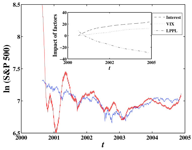
Figure 1: Comparison of the S&P500 index price with the best fit obtained with Eq. (12), Eq. (13) and Eq. (15). The fitted parameter values are the following: $t_{c}={\rm{2000/07/09}}$, $m=0.44$, $\omega=7.83$, $\psi=2.78$, $A=18.70$, $\phi=5.16\times 10^{-4}$, $B=-1.93$, and $C=-0.03$. The inset shows the impact of different factors.

Using Eqs. (13,14,15), we have fitted the USA S&P 500 price in its antibubble regime since year 2000 (see [25, 26, 28, 30] for previous related works on the behavior of the market after the crash of March-April 2000) and the result is shown in Fig. 1. The r.m.s. of the fit residuals is $\chi=0.20$, which is very large compared with the pure LPPL fit, showing that Model 1 is a bad representation of the price.

In addition to the large value of the r.m.s. of the fit residuals, there is another diagnostic for the bad quality of Model 1: the three different contributions (LPPL, VIX and interest rate $r(t)$) are large compared with their sum, suggesting the existence of spurious (in the sense of “over-fitting”) compensations between these terms. In contrast, since the LPPL term was shown to fit very well the data over the period from 2000 to 2003 [25, 26, 28, 30], the LPPL term should be the leading contribution while the other factors should have been perturbations, perhaps growing with time. In other words, Model 1 is not a perturbation of the LPPL model used previously in [25, 26, 28, 30]. And the reason for this is that the interest rate contribution $\int_{t_{0}}^{t}r(\tau){\rm{d}}\tau$ is given and its amplitude cannot be modulated within the RE formulation. Since the risk-free interest rate has been always positive, its integral grows with time, given a contribution with a trend opposite to the overall negative trend of the price over the period 2000 to 2003; hence, the need for the LPPL contribution to counter-balance this effect and the ensuing bad fit and probably strong over-fitting.

3 Model 2: Weaker semi-martingale condition on prices

Generalizing Model 1 to include other factors does not improve, because the positive contribution of the risk-free interest rate (which is an essential component in the RE formulation of the pricing model) requires the other terms and in particular the LPPL component to adjust to large negative values to compensate its large positive contribution. The risk-free interest rate turns out to have an overwhelming and counter trending role in the bearish phase of the market with declining prices. In the context of the RE formalism, a declining price would then require very strong antagonistic forces to compensate, leading to unrealistic impacts of other factors and of the LPPL contribution. Adding other factors do not provide realistic explanations of the price trajectory over this period. We do not show the fits and corresponding figures obtained with all the factors we have tested, as they teach a lesson similar to that of Fig. 1. We conclude that it is essentially impossible to obtain a good model of the empirical price trajectory using the no-arbitrage rational expectation bubble model enriched with factors such as interest rate spread, volatility and exchange rates.

We are thus forced to remove the no-arbitrage condition and replace it by a weaker condition. This amounts to assuming that the market is incomplete. Indeed, we find that the technical source of the problems in fitting the empirical data with our model is the very large cumulative contribution of the risk-free interest rate $r(t)$. Recall that this contribution comes from the no-arbitrage condition obtained under a change of probability measure from the objective to a ‘risk-neutral’ probability measure (a priori distinct from the objective one), which changes the price process from a semi-martingale into a martingale [8, 9]. We thus propose to change the no-arbitrage condition, which is equivalent to requiring that the prices are martingales, by the condition that the prices follow a semi-martingale, with the drift of the semi-martingale taken proportional to the risk-free rate. In the setting of incomplete markets, the fair price is not attainable as the particular expectation over a unique risk-neutral measure, but rather as a supremum over an infinite set of equivalent martingale measures [16]. Our specification for the drift of our semi-martingale price amounts to reducing the set of equivalent measures as in a variational set-up. We allow this drift to adjust its amplitude to reflect the existence of price deviations which have not been arbitraged away, possibly due to technical constraints such as transaction costs and short-sale constraints, but also because of the reluctance of arbitragers to take risks against the crowd sentiments. In other words, the abandon of the no-arbitrage condition reflects the non-fully rational behavior of investors.

The transition to incomplete markets amounts to change (10) into

$$L(t)=\exp\left(\int_{t_{0}}^{t}d\tau\left[\alpha r(\tau)+\phi\sigma(\tau)\right]\right)~{},$$ (16)

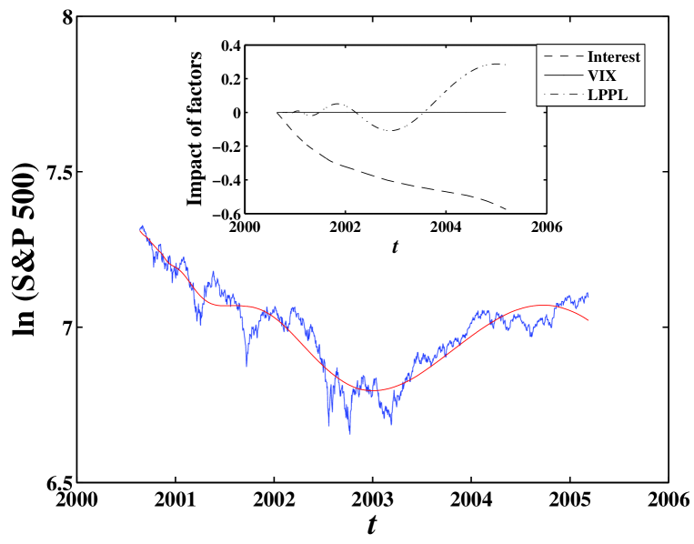
Figure 2: Comparison of the S&P500 index price with the best fit of model 2 defined by expression (9) with (16) and (11). The fitted parameter values are the following: $t_{c}=2000/09/30$; $m=1.22$, $\omega=4.68$, $\psi=3.62$, $\phi=0$, $A=7.32$, $\alpha=-1.58\times 10^{-2}$, $B=4.58\times 10^{-6}$, and $C=3.51\times 10^{-5}$. The r.m.s. of the fit residuals is 0.0482. The inset shows the impact of different factors. The the LPPL factor is reduced or translated by the amount of $A$ for a better comparison.

where $\alpha$ is a new adjustable parameter. Expression (9) with (16) and (11) define our Model 2, whose fit to the price time series of the the S&P500 already shown in Fig. 1 is presented in Fig. 2. The r.m.s. of the fit residuals is $\chi=0.0482$. The improvement of model 2 compared with model 1 is twofold and very significant. First, model 2 better captures the evolution of the S&P 500 index with a much smaller value of the r.m.s. of the fit residuals. Second, the relative amplitudes of the impact of interest and VIX are much smaller than in model 1. However, we see that the impact of VIX is still very large compared with the LPPL factor. This calls for further modification of the model.

4 Addition of other factors

4.1 Description of other potentially relevant factors

The introduction of the price volatility $\sigma(t)$ in Models 1 and 2 of the previous section was justified by the assumed positive relation between risk and return suggested by most asset pricing models [17]. There is a large empirical literature that has tried to establish the existence of such a tradeoff between risk and return for stock market indices. As summarized in [6], the results have been inconclusive and the relation between risk and return is often found insignificant, and sometimes even negative. However, with better monthly variance estimates based on past daily squared returns, the ICAPM intertemporal relation between the conditional mean and the conditional variance of the aggregate stock market return has recently been found positive [5]. One possible reason for the difficulties in measuring a positive risk-return relation is that other state variables in addition to the volatility may influence the investment opportunities anticipated by investors [2, 21]. In particular, variables related to the business cycle have been found to predict returns [3]. They include the dividend-price ratio, the relative Treasury bill rate, the default spread (difference between the yield on BAA and AAA-rated corporate bonds, obtained from the FRED database), the Fama-French factors Rm, SMB, and HML, the exchange rates and so on. The excess return Rm on the market is calculated as the value-weighted return on all NYSE, AMEX, and NASDAQ stocks (from CRSP) minus the one-month Treasury bill rate (from Ibbotson Associates). SMB (Small Minus Big) is the average return on three portfolios made of assets with small capitalizations minus the average return on three portfolios made of assets with big capitalizations. HML (High Minus Low) is the average return on two value portfolios minus the average return on two growth portfolios. In addition, determinants of investors’ risk aversion identified in the asset pricing literature are economic growth prospects, measures of equity and credit market risk, fluctuations in the exchange rate and negative news events in other equity markets. If any of these factors are anticipated to forecast or influence future returns, they should be incorporated in the return equation. We thus discuss extensions of Model 2 which incorporate different additional factors as now explained.

4.2 Model 3: Adding the exchange rate factor

The fact that exchange rates (for instance euro/$, i.e., the value of one euro in dollars) is a relevant factor in the price equation is suggested empirically by a live experiment to forecast the S&P500 index that we have performed from Oct. 2002 till Nov. 2004. This experiment led to the suggestion that the S&P500 index was more predictable when expressed in euros or other major foreign currencies than in US dollars. The rational for this observation is multifold. First the conversion of the dollar value of the US stock market into euros reflects more the view point of foreign investors, which constitute a growing fraction of the population of investors, especially at times of speculative bubbles and more generally herding [27], but also due to the growing influence of debts at times of bulging US deficits. Second, valuing in euro provides a simple mean of eliminating (at least in part) the dollar effect resulting from the policy of the Fed (and in particular its liquidity inputs). Third, the relevance of the exchange rate as an important factor to forecast returns may reflect the expectation that a lower dollar means a more competitive US economy, with its many spillovers on market shares, job creation, earnings, investments and productivity gains and so on. Inversely, a weaker dollar may actually be worrying because it favors the resumption of inflation, higher interest rates which may slow down the economy, potential loss of confidence of foreign investors on the sustainability of the US deficits, varying profits for companies trading internationally and so on. The exchange rate is also responding to global trade deficit of the US versus the rest of the world. It is often advanced that the progressive collapse of the US dollar since 2002 is in large part driven by the growing US deficits (Federal debt, private debt, and current account) [18]. These effects are in general going in opposite directions but with different time scales.

Let us thus write

$$p_{\$}(t)=p_{\rm euro}(t)e^{R_{\rm exch}(t)}~{},$$ (17)

which defines the exchange rate return between the dollar and the euro. Putting for instance $p_{\rm euro}=1$ gives the number of dollars equal to $e^{R_{\rm exch}}$ we obtain from one euro at time $t$. Now, the risk perceived by the economic agents is not determined by $e^{R_{\rm exch}(t)}$ or $R_{\rm exch}(t)$ but by the relative temporal variations of $p_{\$}(t)/p_{\rm euro}(t)$. We have $R_{\rm exch}(t)=\ln p_{\$}(t)-\ln p_{\rm euro}(t)$ and thus

$$r_{\rm exch}(t)\equiv dR_{\rm exch}(t)/dt=\frac{dp_{\$}(t)/dt}{p_{\$}(t)}-\frac{dp_{\rm euro}(t)/dt}{p_{\rm euro}(t)}~{}.$$ (18)

$r_{\rm exch}(t)$ defined in (18) quantifies the real risks due to changes in exchange rates. Indeed, an investor long in dollars (say, he owns one unit of dollars) has the equivalent wealth of $e^{-R_{\rm exch}(t)}$ euros at time $t$, which becomes $e^{-R_{\rm exch}(t+dt)}$ euros at time $t+dt$. He makes a relative profit or loss (return) in euro equal to

$$\frac{e^{-R_{\rm exch}(t+dt)}-e^{-R_{\rm exch}(t)}}{e^{-R_{\rm exch}(t)}}=-r_{\rm exch}(t)dt~{}.$$ (19)

Of course, the situation is symmetric for an investor having one euro and measuring his wealth variation in dollars, leading to a profit or loss of $+r_{\rm exch}(t)dt$ over one elementary time step $dt$.

We thus generalize the market price of risks

$$\phi(t)dW(t)\to\phi dW+\eta_{\rm exch}r_{\rm exch}(t)dW_{\rm exch}~{},$$ (20)

where $\eta_{\rm exch}$ sets the scale of the impact of the risks associated with the exchange rate fluctuations. Note that $\eta_{\rm exch}$ can be either positive or negative. Correlatively, we generalize the price dynamics (5) to make explicit its dependence on the factors identified in the market price of risks:

$$\frac{dp}{p}=\mu(t)dt+\sigma_{p}^{\rm exch}dW_{\rm exch}+\sigma(t)dW-\kappa dj~{}.$$ (21)

The total volatility (variance) of the price returns $[\sigma_{p}^{\rm exch}]^{2}+[\sigma(t)]^{2}$ is the sum of two contributions, one resulting from the fluctuations associated with the exchange rate and the other which captures all other factors of uncertainty. Then, the semi-martingale condition leads to change (8) into

$$\mu(t)=\alpha r(t)+\kappa h(t)+\gamma\sigma(t)+\alpha_{\rm{exch}}r_{\rm exch}(t)~{},$$ (22)

where $\alpha_{\rm{exch}}=\eta_{\rm exch}\sigma_{p}^{\rm exch}$. The expected price conditioned on no crash/rally occurring ($dj=0$) is of the form (9) with

$$\L(t)=\exp\left(\int_{t_{0}}^{t}d\tau\left[\alpha r(\tau)+\gamma\sigma+\alpha_{{\rm{exch}}}r_{\rm{exch}}\right]\right)~{}.$$ (23)

Note that $\gamma\geq 0$, while $\alpha_{\rm exch}$ can be of any sign, depending whether the risk factor is $r_{\rm exch}$ or its negative $-r_{\rm exch}$. The choice of one or the other amounts to analyzing the exchange rate from dollars to euros or vice-versa. This symmetry allows for an a priori arbitrary sign for $\eta_{\rm exch}$.

According to (17) and (18),

$$\int_{t_{0}}^{t}d\tau~{}r_{\rm exch}(t)=\ln\left[\frac{p_{\$}(t)}{p_{\rm euro}(t)}\frac{p_{\rm euro}(t_{0})}{p_{\$}(t_{0})}\right]~{}.$$ (24)

Then, for the special choice $\alpha_{\rm{exch}}=\eta_{\rm exch}\sigma_{p}^{\rm exch}=1$, we have

$$e^{\alpha_{\rm{exch}}\int_{t_{0}}^{t}d\tau~{}r_{\rm exch}(\tau)}=\frac{p_{\$}(t)}{p_{\rm euro}(t)}\frac{p_{\rm euro}(t_{0})}{p_{\$}(t_{0})}~{}.$$ (25)

In this case, expression (9) with $p(t)$ understood as $p_{\$}(t)$ is replaced by

$${\rm E}_{t_{0}}[p_{\rm euro}(t)]=p_{\rm euro}(t_{0})~{}{\hat{L}}(t)~{}\exp\left(\kappa\int_{t_{0}}^{t}d\tau h(\tau)\right)~{},$$ (26)

where

$${\hat{L}}(t)=\exp\left(\int_{t_{0}}^{t}d\tau\left[\alpha r(\tau)+\gamma\sigma(\tau)\right]\right)~{}.$$ (27)

In words, equation (26) means that the term $\exp\left(\int_{t_{0}}^{t}d\tau\left[\alpha_{{\rm{exch}}}r_{\rm{exch}}\right]\right)$ in (23) embodying the exchange risk factor is absorbed in the transformation from dollars to euros. Model 3 thus provides a justification for expressing the US stock market from the view point of the euro as we have done in our monthly online predictions (our monthly predictions used ${\hat{L}}(t)=1$). This procedure is nothing but the particular case ($\alpha_{\rm{exch}}=\eta_{\rm exch}\sigma_{p}^{\rm exch}=1$) of Model 3 which incorporates the risk factor associated with the exchange rates between the US dollar and other currencies. By generalizing the description of the US stock market viewed not solely from the vantage of foreigners, Model 3 allows for a market price of risk associated with the exchange rate which is not entirely described in terms of the euro view point.

We implement Model 3 numerically as:

$$y(t)=A+\alpha r(t)+\gamma v(t)+\alpha_{\rm exch}R(t)+Bf(t)+Cg(t)~{},$$ (28)

where

$$\left\{\begin{array}[]{rcl}y(t)&=&\ln[p(t)]~{},\\ A&=&\ln[p(t_{0})]~{},\\ r(t)&=&\int_{t_{0}}^{t}r_{3m}(\tau){\rm{d}}\tau~{},\\ v(t)&=&\int_{t_{1}}^{t}\sigma(\tau){\rm{d}}\tau~{},\\ R(t)&=&\int_{t_{0}}^{t}r_{\rm{exch}}(\tau){\rm{d}}\tau~{},\\ f(t)&=&(t_{c}-t)^{m}~{},\\ g(t)&=&(t_{c}-t)^{m}\cos[\omega\ln(t_{c}-t)-\phi]~{},\end{array}\right.$$ (29)

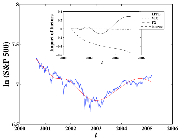
Figure 3: Comparison of the S&P500 index price with the best fit of model 3 defined by expression (9) with (16) and (11). The fitted parameter values are the following: $t_{c}=2000/10/17$; $m=1.25$, $\omega=4.52$, $\psi=4.83$, $\gamma=0$, $A=7.31$, $\alpha=-1.55\times 10^{-2}$, $\alpha_{\rm{exch}}=2.02\times 10^{-2}$, $B=2.68\times 10^{-6}$, and $C=2.98\times 10^{-5}$. The r.m.s. of the fit residuals is 0.0482. The inset shows the impact of different factors. The LPPL factor is reduced or translated by the amount of $A$ for a better comparison.

Figure 3 shows the evolution of the S&P 500 index from Aug-20-2000 to Mar-21-2005 fitted with Model 3. The r.m.s. of the fit residuals is 0.0482. We notice that this figure is undistinguishable from Fig. 2. Both model 2 and model 3 gives the same r.m.s. of fit residuals and the fitted parameters are quite close to each other. In the inset, we see that the impact of the foreign exchange rate can be neglected. Notwithstanding the decrease of the interest rate during the antibubble period, which is causally slaved by the market [29], the short term interest rate has increasing negative impact on the stock market.

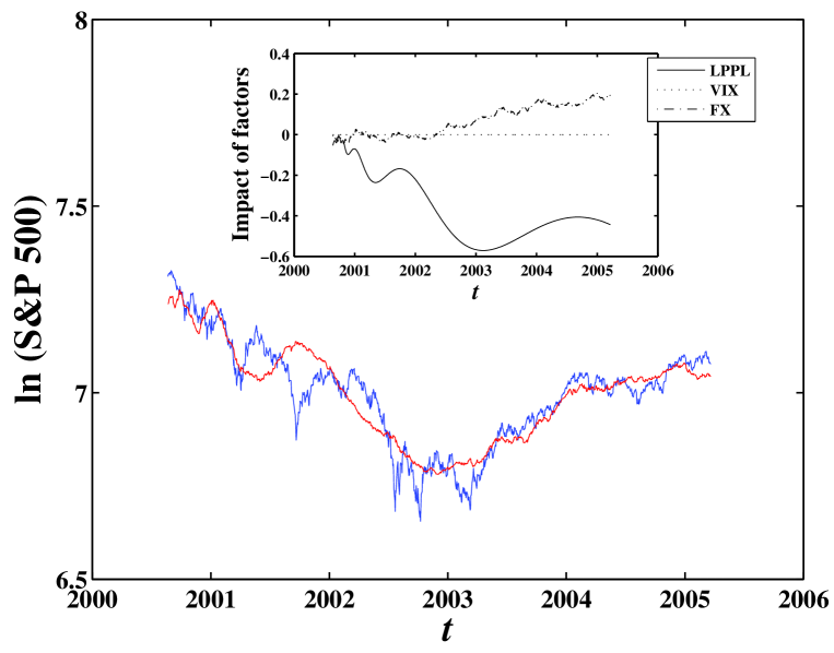
Figure 4: Comparison of the S&P500 index price with the best fit of the modified model 3. The fitted parameter values are the following: $t_{c}=2000/09/25$; $m=0.65$, $\omega=4.60$, $\psi=3.99$, $\gamma=0$, $A=7.29$, $\alpha_{\rm{exch}}=-0.502$, $B=-5.55\times 10^{-3}$, and $C=1.93\times 10^{-3}$. The r.m.s. of the fit residuals is 0.0553. The inset shows the impact of different factors. The LPPL factor is reduced or translated by the amount of $A$ for a better comparison.

From Fig. 3, the impact of interest rate is still very large, we thus fit a modified model 3 containing LPPL, VIX, FX but without the interest rate $r(t)$ (forcing $\alpha=0$). The result is shown in Fig. 4. This new figure emphasizes just the effect of the FX, without the interfering effect of the interest rate $r(t)$ and again the impact of VIX can be neglected.

4.3 Model 4: Semi-Martingale bubble model with additional factors

It is natural to extend Model 2 defined by (9) with (23), by adding other known factors of risks. We explore the relevance of the interest rate spread and of the historical volatility. This amounts to change (23) into

$$\L=\exp\left(\int_{t_{0}}^{t}d\tau\left[\alpha r+\gamma\sigma+\alpha_{\rm exch}r_{\rm exch}+\alpha_{\rm hist}\sigma_{\rm hist}+\alpha_{\rm spread}(r_{\rm{10y}}-r_{\rm{3m}})\right]\right)$$ (30)

where $\alpha_{\rm hist}$ and $\alpha_{\rm spread}$ are two new adjustable parameters. Note again that $\gamma$ and $\alpha_{\rm hist}$ are taken positive. $r_{\rm{10y}}-r_{\rm{3m}}$ is the difference in yields between the Treasury bill with $10$ year and $3$ month maturities.

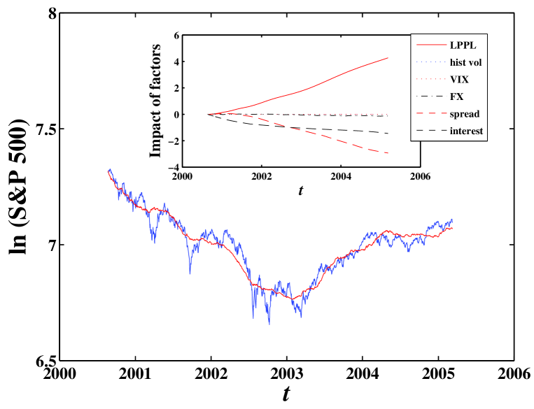
Figure 5: Evolution of the S&P 500 index from Aug-20-2000 to Nov-20-2003 with the fit to Model “weak”. The values of the fit parameters are the following: $t_{c}=2000/09/09$; $m=1.30$, $\omega=7.80$, $\psi=0.82$, $\gamma=0$, $\alpha_{\rm{hist}}=0$, $A=7.31$, $\alpha=-3.89\times 10^{-2}$, $\alpha_{\rm{spread}}=-7.64\times 10^{-2}$, $\alpha_{\rm{exch}}=0.345$, $B=2.83\times 10^{-4}$, $C=9.88\times 10^{-6}$. The r.m.s. of the fit residuals is 0.0409. The inset shows the impact of different factors contributing to the overall fit of Model 4. The LPPL factor is reduced or translated by the amount of $A$ for a better comparison.

Proceeding as before for the OLS fit of this Model 4 to the S&P500 price trajectory, we obtain Fig. 5. The r.m.s. of the fit residual is $0.0409$, which is smaller than the value $0.0436$ of the second-order Landau fit to the same data set (which was up to now the best, i.e., smallest r.m.s) and of course much smaller than the r.m.s. $0.0601$ of fit residuals using the first-order LPPL model. The inset shows the amplitudes of the contributions of the different factors to the global fit. It shows that, in addition to the LPPL factor previously considered in [25, 26, 28, 30], the short-term interest rate and the interest rate spread are the dominant factors, while the other three factors are weaker. The contribution of $\sigma$ (or VIX) and the historical volatility are actually completely negligible since the values of $\gamma$ and $\alpha_{\rm{hist}}$ is very small and close to zero.

Notwithstanding the overall quality of this fit shown in Fig. 5, we argue that it should be disqualified for the same reasons as discussed in section 2.3 concerning Fig. 1: the spread and interest rate contributions are quite large, which forces the LPPL contribution to increase with time. This LPPL contribution thus exhibits a trend opposite to the initial simple LPPL fit and, therefore, Model 4 cannot be considered as a perturbation to the simple LPPL model.

4.4 Second-order Landau formula

An extension of the LPPL formulas (11) and (12) described in section 2.3 has been proposed in [24], based on a formulation of the critical power law behavior in terms of a Landau-like expansion

$$\frac{dF(\tau)}{d\ln\tau}=\alpha F(\tau)+\beta|F(x\tau)|^{2}F(\tau)...~{},$$ (31)

where the coefficients are generally complex and $\tau=|t-t_{c}$. Keeping only the first term $\alpha F(\tau)$ of the right-hand-side of (31) with $\alpha=m+i\omega$ retrieves (13) without the term $\phi v(t)$, which is the so-called first-order LPPL formula [22]. Including the second-order term $\beta|F(\tau)|^{2}F(\tau)$ leads to [24]

$$I(t)=A+\frac{B\tau^{m}+C\tau^{m}\cos\left\{\omega\ln\tau+\frac{\Delta_{\omega}}{2m}\ln\left[1+\left(\frac{\tau}{\Delta_{t}}\right)^{2m}\right]+\phi\right\}}{\sqrt{1+\left(\frac{\tau}{\Delta_{t}}\right)^{2m}}}~{},$$ (32)

which was used to model the bubbles before the USA 1929 crash and 1987 crash [24]. A third order LPPL formula was used to model the nine-year Nikkei antibubble since January 1990 and predict the ensuing two-year evolution [13, 14].

Equation (32) predicts the transition from the angular log-frequency $\omega+\Delta_{\omega}$ for $\Delta_{t}<|t-t_{c}|$ to the angular log-frequency $\omega$ close to $t_{c}$. This corresponds to an approximate description of a log-frequency modulation. For instance, the 1990 Nikkei antibubble studied in [13, 14] experienced the transition from the first-order Landau description (11) and (12) to the second-order Landau formula (32) approximately 2.5 years after the inception of the antibubble [13, 14]. In contrast, the 2000 S&P 500 antibubble was found to just barely enter the second-order Landau regime on the fourth quarter of 2003 after more three years since its inception [30], while the second-order Landau regime was undetectable from data ending in the last quarter of 2002 [26].

In the following tests, we compare between them the different models constructed with different factors and with the second-order LPPL formula (32).

5 Tests on the relevance of the different factors

Let us consider the family of one-factor LPPL models defined by

$$\L=\exp\left(\int_{t_{0}}^{t}\alpha_{i}f_{i}d\tau\right),~{}{\rm{with}}~{}i=1,2,3,4,{\rm{and}}~{}5,$$ (33)

where $\alpha_{1}f_{1}=\alpha r$, $\alpha_{2}f_{2}=\gamma\sigma$, $\alpha_{3}f_{3}=\alpha_{\rm exch}r_{\rm exch}$, $\alpha_{4}f_{4}=\alpha_{\rm hist}\sigma_{\rm hist}$, and $\alpha_{5}f_{5}=\alpha_{\rm spread}(r_{\rm{10y}}-r_{\rm{3m}})$. We fit the S&P 500 antibubble after the burst of the “new economy” bubble in April of 2000 using each of the five models defined by Eq.(33). The time series is fitted from Aug-20-2000 to a time $t_{\rm{last}}$ which is varied from 08-Apr-2002 to 10-Mar-2005 with a step of 21 trading days. Each interval from Aug-20-2000 to a time $t_{\rm{last}}$ is fitted by each of the five models.

5.1 Akaike’s AIC criterion

To compare these five models with the first-order LPPL and second-order LPPL, we use Akaike’s minimum AIC estimation [1], which was designed for the identification of several competing models. The AIC is defined by

$${\rm{AIC}}=-2\ln(L)+2\kappa~{},$$ (34)

where $L$ is the maximum likelihood of a given model given the data and $\kappa$ is the number of independently adjusted parameters within a model. By assuming a Gaussian distribution of the fit residuals, we have

$$\ln L=-n\ln(\hat{\sigma})-\frac{n}{2}[\ln(2\pi)+1]~{},$$ (35)

where $n$ is the number of data points and $\hat{\sigma}^{2}=\chi^{2}$ is the maximum likelihood estimate of the variance of the fit residual.

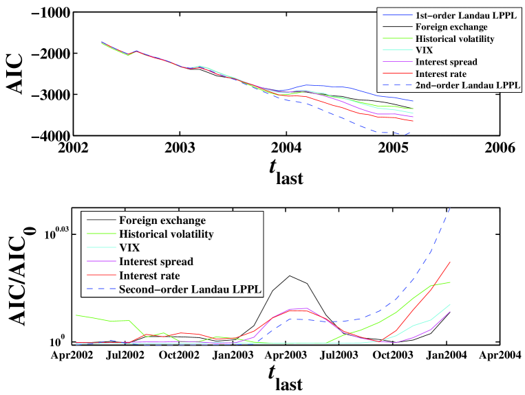
Figure 7: (Top panel) AIC of the five one-factor LPPL models with comparison to the first- and second-order Landau LPPL models. (Bottom panel) Relative AIC against the AIC₀ of the first-order LPPL model.

The top panel of Fig. 7 shows the evolution of the AIC’s of the five one-factor LPPL models in comparison with the first- and second-order Landau LPPL models. To better illustrate the competition among the models, we plot the relative AIC with respect to the first-order LPPL model in the lower panel of Fig. 7. This figure suggests that the historical volatility played the key role before August of 2002. Around October 2002, the interest rate dominated. In the first six months of 2003, the foreign exchange rate became the key factor. Since the end of 2003, all factors have played an increasingly large role. Note also that after July 2003, the second-order Landau LPPL model has the largest AIC and is identified as the best model, suggesting as discussed elsewhere [25, 30] a progressive maturation of the herding effect in this “antibubble,” similarly to the case of Japan [12, 14].

We should stress however that this qualitative similarity between the US antibubble since 2000 and the Japanese antibubble since 1990 does not extend to the quantitative level. In [26] written in 2003, we stated that we could not find neither quantitative nor qualitative differences between the US and the JP antibubbles. Things have changed in the last two years. Our present analysis shows that the second-order LPPL regimes of the two antibubbles are quite different; for instance, the important parameter $\Delta\omega$ have different signs and significantly different values; the $\Delta_{t}$ ’s are also very different. We conjecture that these quantitative differences may signal deep divergences in the mechanisms and evolutions of the two antibubbles in the present regime described by the second-order LPPL model and beyond.

5.2 Wilks’ test of embedded hypotheses

Since the single factor models defined with expression (33) contain Model 1 defined by (13) as a special case $\alpha_{i}=0$, we can use Wilks theorem [20] and the statistical methodology of nested hypotheses to assess whether the hypothesis that $\alpha_{i}=0$ can be rejected. By assuming a Gaussian distribution of observation errors (residuals) at each data point, the maximum likelihood estimation of the parameters amounts exactly to the minimization of the sum of the square over all data points (of number $n$) of the differences $\delta_{j}(i)$ between the mathematical formula and the data [19]. According to Wilks theorem of nested hypotheses, the log-likelihood-ratio

$$T=-2(L_{0}-L_{1})=2n(\ln\sigma_{1}-\ln\sigma_{0})~{},$$ (36)

is a chi-square variable with $k$ degrees of freedom, where $k$ is the number of restricted parameters [7]. In the present case, we have $k=1$. The Wilks test thus amounts to calculate the probability that the obtained value of $T$ can be over-passed by chance alone. If this probability is small, this means that chance is not a convincing explanation for the large value of $T$ which becomes meaningful. This implies a rejection of the hypothesis that $\alpha_{i}=0$ is sufficient to explain the data and favor the fit with $\alpha_{i}\neq 0$ as statistically significant.

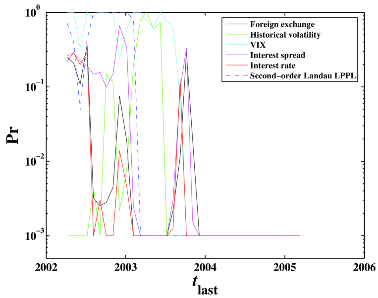
Figure 8: Wilks’ log-likelihood-ratio test of the significance of the new factors introduced in (33). The second-order Landau formula is also tested. Note that all values of $\rm{Pr}$ which are less than 0.001 are plotted to be 0.001 in the figure for better representation.

Figure 8 plots the evolution of the probability ${\rm{Pr}}$ that the log-likelihood-ratio exceeds $T$ at $t_{\rm{last}}$. The second-order Landau formula is also tested for comparison. We see that there are always factors that are significant at a level of significance far better than 99%, that is, ${\rm{Pr}}<1\%$. For instance, $\alpha_{4}\neq 0$ (historical volatility) passed the test in the time period before August of 2002. Since 2004, all five one-factor models and the second-order Landau model are significant.

It is noteworthy that the second-order Landau formula experienced a transition from large ${\rm{Pr}}$ to small ${\rm{Pr}}$ in the first quarter of 2003, signaling the crossover from the first-order Landau regime to the second-order regime, which confirms our earlier preliminary assessment [30]. In contrast, the one-factor models exhibit large values of ${\rm{Pr}}$ for several months in 2003.

Together with the fact that the r.m.s. of the residues of the fit is the smallest for the second-order LPPL formula (32), we conclude that the second-order LPPL model is the best model. The economic factors investigated here seem less powerful than just herding effects to account for the continuation of the unraveling of the US stock market antibubble.

6 Prediction using the second-order LPPL formula (32)

So far, we have shown that the macroscopic factor models are not as good as the second-order formula. For the US S&P 500 antibubble started in August 2000, the second-order formula (32) provides by far the best model so that the other factors cannot explain what is going on in the US stock market. Our analysis also shows that the antibubble has entered the second-order Landau regime approximately during the summer of 2003, confirming our preliminary analysis [29]. In addition, the tests in [29] showed that, in the framework of the first-order Landau model, the antibubble was probably still alive in August 2003 but has ended since in the USA (i.e., when viewed from the view point of a US investor valuing in US dollars). The timing of the end of the first-order LPPL antibubble is roughly consistent with our current analysis.

To further show that the crossover happened in 2003, we show in Fig. 9 the evolution of the fitted values of $\Delta_{t}$ and $\Delta_{\omega}$ which are the diagnostic of the relevance of the second-order formula. The dramatic drop of the value of $\Delta_{t}$ endorses the crossover from the first-order regime to the second-order.

These tests suggest that it is possible to resume the modeling and prediction of the antibubble within the second-order Landau model. Fig. 10 shows the fit of the US S&P 500 index from $2000/08/21$ to $2005/03/21$ using the second-order Landau formula. The fitted inception date of the antibubble $t_{c}=2000/08/17$ is found stable in all our fits with different terminal values of the fitted windows. The extrapolation of the fitted second-order formula shown in Fig. 10 suggests that the market is not yet ready for a solid recovery.

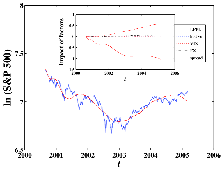
Figure 6: Fit to the modified model of all factors except the interest rate. The values of the fit parameters are the following: $t_{c}=2000/07/16$; $m=0.80$, $\omega=5.44$, $\psi=4.17$, $\gamma=0$, $\alpha_{\rm{hist}}=9.11\times 10^{-7}$, $A=7.39$, $\alpha_{\rm{spread}}=1.54\times 10^{-2}$, $\alpha_{\rm{exch}}=-0.182$, $B=-3.23\times 10^{-3}$, and $C=5.84\times 10^{-4}$. The r.m.s. of the fit residuals is 0.0517. The inset shows the impact of different factors contributing to the overall fit of Model 4. The LPPL factor is reduced or translated by the amount of $A$ for a better comparison.

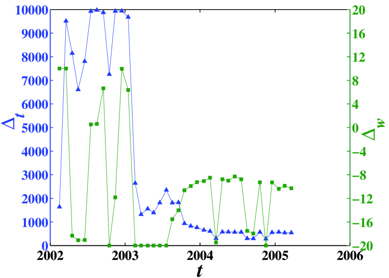
Figure 9: The evolution of the fitted values of $\Delta_{t}$ and $\Delta_{\omega}$. The dramatic drop of the value of $\Delta_{t}$ endorses the crossover from the first-order regime to the second-order.

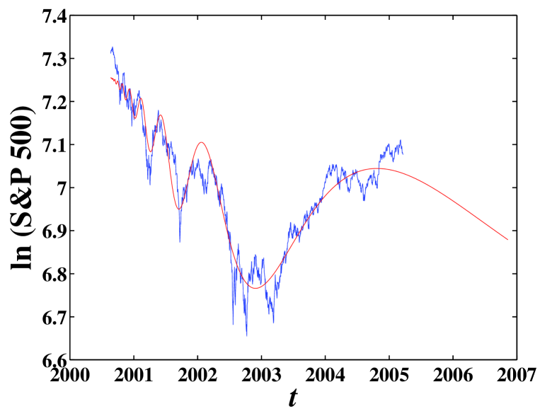
Figure 10: Modeling and prediction of the US S&P 500 index from $2000/08/21$ to $2005/03/21$ using the second-order Landau formula (32). The fitted parameters are $t_{c}=2000/08/17$, $m=1.32$, $\omega=13.72$, $\psi=1.31$, $\Delta_{t}=545$, $\Delta_{\omega}=-10.28$, $A=7.26$, $B=-9.505\times 10^{-5}$, and $C=-4.224\times 10^{-5}$ with the r.m.s. of fit residuals being 0.0403.

References

- [1] Akaike, H., A new look at the statistical model indentification, IEEE Transactions on Automatic Control 19, 716 (1974).
- [2] Campbell, J.Y., Intertemporal asset pricing without consumption data , American Economic Review 83, 487-512 (1993).
- [3] Campbell, J.Y., A.W. Lo, and A.C. MacKinlay, The Econometrics of Financial Markets (Princeton University Press: Princeton, 1997).
- [4] Cochrane, J.H., Asset Pricing, (Princeton University Press, Princeton, 2001)
- [5] Ghysels, E., P. Santa-Clara and R. Valkanov, There is a Risk-Return Tradeoff After All, Journal of Financial Economics, forthcoming.
- [6] Goyal, A. and P. Santa-Clara, Idiosyncratic risk matters! The Journal of Finance 58 (3), 975-1007 (2003).
- [7] Holden K, Peel DA and Thompson JL, Economic Forecasting: An Introduction (Cambridge University Press, Cambridge, 1990) pp.59.
- [8] Harrison, J.M. and D.M. Kreps, Martingales and arbitrage in multiperiod securities markets, Journal of Economic Theory, 20 (3), 381-408 (1979).
- [9] Harrison, J.M., and S.R. Pliska, Martingales and stochastic integrals in the theory of continuous trading, Stochastic Processes and their Applications, 11, 215-260 (1981).
- [10] Johansen, A. and Ledoit, O. and Sornette, D., Crashes as critical points, International Journal of Theoretical and Applied Finance 3, 219-255 (2000).
- [11] Johansen, A and Sornette, D, Critical crashes, Risk 12, 91-94 (1999).
- [12] Johansen, A. and D. Sornette, Financial “anti-bubbles”: log-periodicity in Gold and Nikkei collapses, Int. J. Mod. Phys. C 10(4), 563-575 (1999).
- [13] A. Johansen and D. Sornette, Financial “anti-bubbles”: log-periodicity in Gold and Nikkei collapses, Int. J. Mod. Phys. C 10, 563-575 (1999).
-
[14]
Johansen, A. and D. Sornette
Evaluation of the quantitative prediction of a trend reversal on the Japanese stock market in 1999, Int. J. Mod. Phys. C Vol. 11 (2), 359-364 (2000) - [15] Johansen, A and Sornette, D and Ledoit, O, Predicting financial crashes using discrete scale invariance, Journal of Risk 1, 5-32 (1999).
- [16] King, A. and L. Korf, Martingale pricing measures in incomplete markets via stochastic programming duality in the dual of , submitted to Mathematics of Operations Research, 2002 (preprint available at http://www.math.washington.edu/~korf/abstracts.html)
- [17] Merton, R.C., An intertemporal capital asset pricing model, Econometrica 41, 867-887 (1973).
- [18] Obstfeld, M. and Rogoff, K., The Unsustainable US Current Account Position Revisited, NBER Working Paper No. 10869 (2004).
- [19] Press, W., S. Teukolsky, W. Vetterling and B. Flannery, Numerical Recipes in FORTRAN: The Art of Scientific Computing (Cambridge University, Cambridge, 1996).
- [20] Rao C, Linear statistical Inference and Its Applications (New York, Wiley, 1965) ch 6, section 6e.3.
- [21] Scruggs, J.T., Resolving the puzzling intertemporal relation between the market risk premium and conditional market variance: A two-factor approach, Journal of Finance 52, 575-603 (1998).
- [22] Sornette, D., Why Stock Markets Crash (Critical Events in Complex Financial Systems) Princeton University Press, January (2003).
- [23] Sornette, D., Endogenous versus exogenous origins of crises, in the monograph entitle “Extreme Events in Nature and Society,” S. Albeverio, V. Jentsch and H. Kantz, eds. (Springer, 2005) (http://arxiv.org/abs/physics/0412026)
- [24] Sornette, D. and A. Johansen, Large financial crashes, Physica A 245, 411-422 (1997).
- [25] Sornette, D. and W.-X. Zhou, The US 2000-2002 Market descent: how much longer and deeper? Quantitative Finance 2 (6), 468-481 (2002).
- [26] Sornette, D. and W.-X. Zhou, The US 2000-2003 Market descent: clarifications, Quantitative Finance 3 (3), C39-C41 (2003).
- [27] Sornette, D. and W.-X. Zhou, Evidence of fueling of the 2000 new economy bubble by foreign capital inflow: implications for the future of the US economy and its stock market, Physica A 332, 412-440 (2004).
- [28] Zhou, W.-X. and D. Sornette, Renormalization group analysis of the 2000-2002 anti-bubble in the US S&P 500 index: Explanation of the hierarchy of five crashes and Prediction, Physica A 330, 584-604 (2003).
- [29] Zhou, W.-X. and D. Sornette, Causal slaving of the U.S. treasury bond yield antibubble by the stock market antibubble of August 2000, Physica A 337, 586-608 (2004).
- [30] Zhou, W.-X. and D. Sornette, Testing the stability of the 2000-2003 US stock market “antibubble”, Physica A 348, 428-452 (2005).