A Simple General Solution for Maximal Horizontal Range of Projectile Motion

Abstract

A convenient change of variables in the problem of maximizing the horizontal range of the projectile motion, with an arbitrary initial vertical position of the projectile, provides a simple, straightforward solution.

I Introduction

A clear, concise formulation of the general solution for maximal horizontal range of the projectile motion is considered non-trivial. Consequently much effort has been spent to formulate a solution that would be understandable to as wide audience as possible. The problem may be stated as follows:

1. Find the maximal horizontal range, $R$, of a projectile launched with an initial speed $v_{0}$ from the point with the vertical coordinate $y_{0}$. (Figure 1)

Generally the known solutions are divided into those that do and those that do not make use of calculus. Somewhat misleadingly the former are commonly qualified as simple. The categorization according to whether a solution starts from the vector or scalar general solution of projectile motion seems more appropriate.

In the former one starts from

$$\begin{split}\vec{r}&=\vec{r_{0}}+\vec{v_{0}}t+\frac{1}{2}\vec{g}t^{2}\\ \vec{v}&=\vec{v_{0}}+\vec{g}t\end{split}$$ (1)

and employs “ingenious application of vector algebra, involving both dot and cross products” (citation from Thomsen J.S.Thomsen (1984)). An example of a solution from this category is given by Palfy-Muhoray and Balzarini P.Palfy-Muhoray and D.Balzarini (1982). While it does not involve calculus the solution can hardly be considered simple. The use of vector algebra as the means for the solution seems to be be inspired by the paper of Winans J.G.Winans (1961) who provided a solution by using quaternion multiplication.

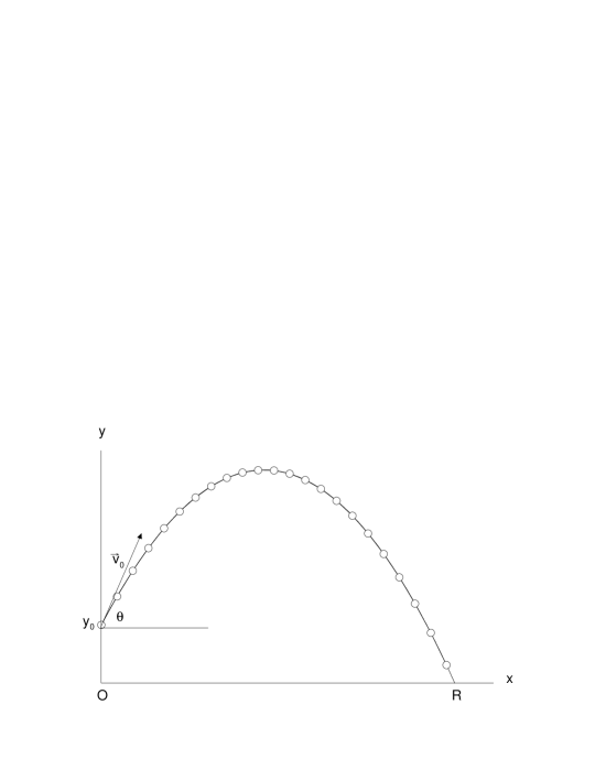
Figure 1: The trajectory of a body projected from the height $y_{0}$ with an initial velocity $\vec{v_{0}}$ at an angle $\theta$ with respect to the horizontal. $R$ is the horizontal range of the motion.

In the latter approach one starts from the more familiar parametric representation of the projectile trajectory

$$\begin{split}x&=v_{0}t\cos{\theta}\\ y&=y_{0}+v_{0}t\sin{\theta}-\frac{1}{2}gt^{2}.\end{split}$$ (2)

The calculus-based solutions (e.g. W.S.Porter (1977); D.B.Lichtenberg and J.G.Wills (1978)) proceed with the substitutions,

$$y=0,\qquad x=R,\qquad t=\frac{R}{v_{0}\cos{\theta}},$$ (3)

and look for the maximum of the resulting function $R=R(\theta)$ by setting

$$dR/d\theta=0.$$ (4)

Lichtenberg and Wills D.B.Lichtenberg and J.G.Wills (1978), to whom this method is usually attributed, maximize

$$R=\frac{v_{0}^{2}}{g}\cos{\theta}\bigg{[}\sin{\theta}+\sqrt{\sin^{2}{\theta}+\frac{2gy_{0}}{v_{0}^{2}}}\bigg{]}.$$ (5)

While the method is straightforward and therefore may be considered simple, the function (5) is quite complicated and the application of the necessary condition for the extremum of a function of one variable (4) leads to a very involving calculation. This may be the main reason to look for the solutions that do not involve calculus.

The substitutions (3) accompanied with the use of the trigonometric identity

$$\frac{1}{\cos^{2}{\theta}}=1+\tan^{2}{\theta}$$ (6)

give

$$0=y_{0}+R\tan{\theta}-\frac{gR^{2}}{2v_{0}^{2}}(1+\tan^{2}{\theta}),$$ (7)

which is the basis for a couple of interesting non-calculus-based solutions. Thomsen J.S.Thomsen (1984), for example, considers Equation (7) as a quadratic equation in $\tan{\theta}$. The requirement that the solutions of the equation be real then leads to a solution of the problem. Baće et al.M.Baće et al. (2002) take the same view of Equation (7) but obtain the solution through a more pointed observation that the maximal horizontal range, $R_{max}$, is realized for the unique initial direction of the projectile.

Some additional solutions are discussed in Brown R.A.Brown (1992), who also gives his own, non-calculus-based solution based on the solution of a related problem of the range of a projectile launched down an incline.

II Change of Variable Solution

Instead of focusing on some explicit relation between the relevant variables, e.g. $R=R(\theta)$ or $R=R(t)$, one can notice that the Equation (7) can be cast in the form where $R^{2}$ is expressed as a quadratic function of $R\medspace\tan{\theta}$,

$$R^{2}=-(R\medspace\tan{\theta})^{2}+2\frac{v_{0}^{2}}{g}(R\medspace\tan{\theta})+2\frac{v_{0}^{2}y_{0}}{g}.$$ (8)

This observation makes both, calculus-based and purely algebraic, solutions simple.

In the former case

$$dR^{2}/d(R\tan{\theta})=0$$ (9)

is equivalent to

$$R_{max}\tan{\theta_{max}}=\frac{v_{0}^{2}}{g}.$$ (10)

Equation (8) then gives

$$R_{max}=\frac{v_{0}}{g}\sqrt{v_{0}^{2}+2gy_{0}},$$ (11)

which in turn, inserted into Equation (10), leads to

$$\tan{\theta_{max}}=\frac{v_{0}}{\sqrt{v_{0}^{2}+2gy_{0}}}.$$ (12)

This completes the solution.

If, on the other hand, an algebraic solution is preferred one can transform Equation (8) into

$$R^{2}-\bigg{[}2\frac{v_{0}^{2}y_{0}}{g}+\frac{v_{0}^{4}}{g^{2}}\bigg{]}=-\bigg{[}R\medspace\tan{\theta}-\frac{v_{0}^{2}}{g}\bigg{]}^{2}$$ (13)

and notice that the right-hand side is non-positive. Thus

$$R^{2}-\bigg{[}2\frac{v_{0}^{2}y_{0}}{g}+\frac{v_{0}^{4}}{g^{2}}\bigg{]}\leq 0,$$ (14)

and

$$R_{max}^{2}=\frac{v_{0}^{2}}{g^{2}}\big{(}v_{0}^{2}+2gy_{0}\big{)}$$ (15)

at

$$R_{max}\medspace\tan{\theta_{max}}=\frac{v_{0}^{2}}{g}.$$ (16)

The last two expressions then lead to (11) and (12).

III Conclusion

The present solution of the problem of maximizing the horizontal range of the projectile motion is based on the widely applicable technique of change of variables. Although this may be implicit in the algebraic variant of the solution, both variants may serve as an illustration of the usefulness of the technique in simplifying otherwise complicated calculations.