Microfluidic capturing-dynamics of paramagnetic bead suspensions

Abstract

We study theoretically the capturing of paramagnetic beads by a magnetic field gradient in a microfluidic channel treating the beads as a continuum. Bead motion is affected by both fluidic and magnetic forces. The transfer of momentum from beads to the fluid creates an effective bead-bead interaction that greatly aids capturing. We demonstrate that for a given inlet flow speed a critical density of beads exists above which complete capturing takes place.

I Introduction

Recently, there has been an increasing interest in using magnetic beads in separation of, say, biochemical species in microfluidic systems Choi et al. (2003); Pankhurst et al. (2003). The principle is to have biochemically functionalized polymer beads with inclusions of superparamagnetic nanometersize particles of, for example, magnetite or maghemite. They attach to particular biochemical species and can be separated out from solution by applying external magnetic fields. As most biological material is either diamagnetic or weakly paramagnetic, this separation is specific. Paramagnetic particles in fluids are also used to measure the susceptibility of, for example, magnetically labelled cells by measuring particle capture or motion in a known field Zborowski et al. (2003); McCloskey et al. (2003).

In this paper we study microfluidic capturing of paramagnetic beads from suspension by modeling the beads as a continuous distribution Warnke (2003). The separation of suspended paramagnetic beads from their host fluid is an important process as it decides operating characteristics for practical microfluidic devices. It involves an interplay between forces of several kinds governing the dynamics of the process: (a) Magnetic forces from the application of strong magnetic fields and field gradients. (b) Drag forces due to the motion of the beads with respect to the host fluid. (c) The trivial effect of gravity, which we ignore in the following. We emphasize the effects of bead motion on the fluid flow as this gives rise to a hydrodynamic interaction between the beads. As we have noted in a previous few-bead study, this interaction is more important than the magnetic bead-bead interactions Mikkelsen et al. (2005). It is created by drag forces in two steps: First, drag transfers momentum to the fluid from the beads moving under the influence of external forces. Second, the modified flow changes the drag on and thus motion of other beads.

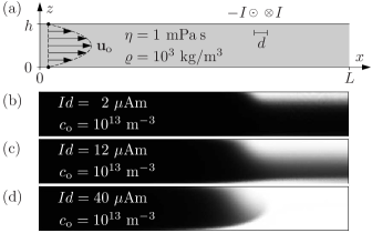
Figure 1: (a) Sketch of the microfluidic system with $L=350~{}\mu$m and $h=50~{}\mu$m. A suspension of paramagnetic beads enters at $x=0$ with a parabolic Poiseuille flow profile, $\mathbf{u}_{\text{o}}$, and leaves at $x=L$. Beads are caught by the pair of wires placed $100~{}\mu$m from the outlet at the top and carrying currents $\pm I$. (b)–(d) Simulated stationary density of the beads ranging from zero (white) to $c_{\text{o}}$ (black) for increasing values of the current-distance product $Id$ as indicated. At $x=0$ the concentration is $c_{\text{o}}=10^{13}$ m^-3 and the maximum flow speed is $300~{}\mu$m/s.

II Model

As sketched in Fig. 1(a) we consider a viscous fluid (water) flowing in the $x$ direction between a pair of parallel, infinite, planar walls. The walls are placed parallel to the $xy$ plane at $z=0$ and $z=h$, respectively. A steep magnetic field gradient is generated by a parallel pair of closely spaced, infinitely long, thin wires along the $y$ direction separated by $d$ and carrying opposite currents $\pm I$. The system is translation invariant in the $y$ direction thereby reducing the simulation to a tractable problem in 2D. The simulation domain is defined by $0<x<L$ and $0<z<h$ with $L=350~{}\mu$m and $h=50~{}\mu$m. The wires intersect the $xz$ plane near $(x,z)=(250~{}\mu\text{m},\ 55~{}\mu\text{m})$ just above the top plate. Paramagnetic beads in suspension are injected into the microfluidic channel by the fluid flow at $x=0$. They are either exiting the channel at $x=L$ or getting collected at the channel wall near the wires.

When a suspension of beads is viewed on a sufficiently large scale compared to the single bead radius $a$ but on a scale comparable to density variations, we can describe the distribution of beads in terms of a continuous, spatially varying bead number density $c$. We consider a suspension of beads with radius $a=1~{}\mu$m and denote the initial number density at $x=0$ by $c_{\text{o}}$. The four basic constituents of the model are described in the following.

Magnetic force. The beads are paramagnetic with a magnetic susceptibility $\chi=1$. In an external magnetic field $\textbf{H}_{\text{ext}}(\textbf{r})$ the force on such a bead is

$$\textbf{F}_{\text{ext}} =\mu_{\text{o}}\!\int_{\text{bead}}(\textbf{M}\cdot\boldsymbol{\nabla})\textbf{H}_{\text{ext}}\,dV$$

$$=4\pi\mu_{\text{o}}a^{3}\frac{\chi}{\chi+3}(\textbf{H}_{\text{ext}}\cdot\boldsymbol{\nabla})\textbf{H}_{\text{ext}}$$ (1)

assuming that the bead is so small that we can take the external field $\textbf{H}_{\text{ext}}$ to be approximately constant across the bead, i.e., $a|\boldsymbol{\nabla}\textbf{H}_{\text{ext}}|\ll|\textbf{H}_{\text{ext}}|$ when determining the magnetization M.

As mentioned, $\textbf{H}_{\text{ext}}$ in this study arises from a pair of current carrying wires. It is determined in the following manner. From Ampère’s law, we readily find the magnetic field, H, around a straight circular wire, $\textbf{H}(\textbf{r})=\textbf{J}\times\textbf{r}/(2\pi r^{2})$, where the electrical current vector J is along the wire orthogonal to the position vector r which is in the $xz$ plane. The magnetic field from the two closely spaced anti-parallel wires is found by decreasing the separation $d$ and increasing the current, $I=|\textbf{J}|$, while keeping the product $Id$ constant,

$$\textbf{H}_{\text{ext}}=\frac{1}{2\pi r^{2}}\left(\textbf{J}\times\textbf{d}-\frac{2(\textbf{J}\times\textbf{r})(\textbf{d}\cdot\textbf{r})}{r^{2}}\right).$$ (2)

This together with Eq. (1) yields

$$\textbf{F}_{\text{ext}}=-\frac{2}{\pi}\frac{\chi}{\chi+3}\mu_{\text{o}}a^{3}(I\,d)^{2}\,\frac{\textbf{r}}{r^{6}}\>;$$ (3)

a manifestly attractive central force (from the mid-point of the wires), independent of the direction of d.

Fluid flow. The beads are suspended in a fluid of viscosity $\eta$ and density $\varrho$ that is launched at $x=0$ with a parabolic velocity profile, $\mathbf{u}_{\text{o}}$, and flows past the wires. In microfluidics inertial effects are unimportant compared to drag, so the small beads in suspension almost always move with constant velocity relative to the fluid. Except for acceleration phases shorter than microseconds the external forces are exactly balanced by drag Newton2 . The momentum transfer from beads to fluid is included by adding a bulk force term, $c\textbf{F}_{\text{ext}}(\textbf{r})$ to the Navier–Stokes equation. This bulk force term is proportional to the number density $c$ of beads and the magnetic external force $\textbf{F}_{\text{ext}}$ on an individual bead at position r. The velocity u of the fluid is given by

$$\varrho\partial_{t}\textbf{u}+\varrho(\textbf{u}\cdot\boldsymbol{\nabla}){\textbf{u}}=-\boldsymbol{\nabla}p+\eta\nabla^{2}\textbf{u}+c\textbf{F}_{\text{ext}},$$ (4)

along with the incompressibility condition $\boldsymbol{\nabla}\cdot\textbf{u}=0$.

Bead motion. To complete the set of equations, it is necessary to have an equation of motion for the bead number density $c$. As the beads neither appear nor disappear in the bulk, $c$ must obey a continuity equation

$$\partial_{t}c+\boldsymbol{\nabla}\cdot\textbf{j}=0,$$ (5)

where the bead current j is defined by the Nernst–Planck equation Probstein (1994)

$$\textbf{j}=-D\boldsymbol{\nabla}c+c\textbf{u}+cb\textbf{F}_{\text{ext}}$$ (6)

with diffusivity $D$ and bead mobility $b=1/(6\pi\eta a)$.

For our spherical beads the diffusivity is given by the Einstein expression $D=kT/(6\pi\eta a)$ which for water at room temperature equals $2.2\times 10^{-13}~{}$m²/s. In the simulations below, however, we artificially increase the magnitude of $D$ in order to stabilize the computations and to use a coarser mesh and thus save computation time.

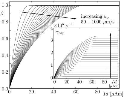
Figure 2: The fraction $\beta$ of beads caught as function of the current-distance product $Id$ for twenty different flow speeds (50 – 1000 $\mu$m/s; indicated by the arrows). Larger current leads to higher $\beta$; faster flow to smaller $\beta$. In this simulation the initial concentration is low, $c_{\text{o}}=10^{13}$ m^-3. Inset: Rate $\gamma_{\text{cap}}$ of bead capture as function of $Id$, for the flows above. The faster flow or the larger current, the higher $\gamma_{\text{cap}}$.

Boundary conditions. In addition to the bulk equations (4), (5), and (6), we need appropriate boundary conditions. As the beads move out to the walls of the domain and settle there, merely demanding that the normal component of the bead current vector j vanishes is not correct, rather, it must be free to take on any value as long as it is directed into the wall. As beads do not enter the bulk from the walls (by assumption once settled, beads stick) we demand that the normal current component is never directed into the liquid. For the fluid we demand the usual no-slip condition at the walls.

At the inlet $x=0$ of the microfluidic channel we assume that the fluid comes in with the constant initial number density $c_{\text{o}}$ and with a parabolic fluid velocity profile $\mathbf{u}_{\text{o}}$. At the outlet $x=L$ we let the bead current take on any value, while the fluid pressure is zero.

III Results

Having set up the equations for bead and fluid motion, they are solved with the finite element method on a mesh with $\sim 10^{4}$ elements refined in the vicinity of the wires. To this end we employ the finite element solver software package Femlab Femlab . The parameter values for the fluid are those of water, $\eta=1$ mPa s and $\varrho=10^{3}$ kg/m³, while for the beads $a=1~{}\mu$m and $c_{\text{o}}=10^{13}$ to $10^{16}$ m^-3.

To study capturing we must keep track of which beads are captured and which are flushed through the channel with the flow. This is done by calculating the rates $\gamma_{i}$ by which the beads are either captured or transported in/out at each of the four boundary segments $i$ of the channel (inlet, outlet, upper wall, and lower wall). By integration of the normal components of the bead currents along each segment $i$, we find

$$\gamma_{i}=\int_{i}\textbf{j}\!\cdot\!\textbf{n}\>d\ell_{i}.$$ (7)

The rate of capture is $\gamma_{\text{cap}}=\gamma_{\text{lower}}+\gamma_{\text{upper}}$. In steady state the conservation of beads enforces $\gamma_{\text{inlet}}+\gamma_{\text{cap}}+\gamma_{\text{outlet}}=0$, which provides a useful check of the simulation results. The primary control parameters are the current-wire distance product $Id$, the maximum fluid in-flow speed $u_{\text{o}}$, and the bead number density, $c_{\text{o}}$. The product $Id$ decides the magnetic force which captures the beads against the fluid flow. As we are investigating effects of bead-bead interaction, our interest is properties that depend on the bead number density, in particular those that do so nonlinearly.

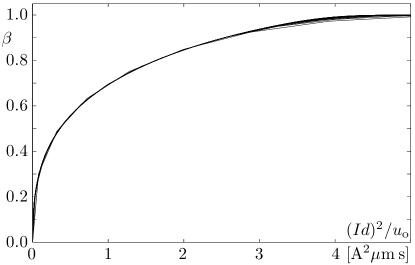
Figure 3: The fraction $\beta$ of beads caught versus $(Id)^{2}/u_{\text{o}}$, the ratio of the current-distance product squared and the fluid flow velocity. This demonstrates scaling in the competition between capturing and flushing: the twenty curves from Fig. 2 approximately collapse to one single.

Electrical current and fluid flow. The effects of having electrical wires near, and thus a magnetic field gradient in, the channel is illustrated in Fig. 1(b)–(d) for three values of the current-distance product $Id$. At small values of $Id$ only a narrow region is emptied but increasing the current the region expands until it covers the width of the channel.

A simple measure of the capturing is the ratio $\beta$ of the bead capture rate $\gamma_{\text{cap}}$ to the bead in-flow rate $\gamma_{\text{inlet}}$,

$$\beta=\frac{\text{``capture rate''}}{\text{``in-flow rate''}}=\frac{\gamma_{\text{cap}}}{\gamma_{\text{inlet}}}.$$ (8)

If capturing dominates $\beta$ tends to unity, if flushing dominates $\beta$ tends to zero. Fig. 2 shows this in that slow flow and strong current leads to a high $\beta$ whereas fast flow and weak current leads to a small value. The rate $\gamma_{\text{cap}}$ of bead capture as function of wire current and flow velocity is illustrated in the inset of Fig. 2.

If there is a competition between magnetic capturing and flushing, then we expect that the data can be described essentially by the ratio of the magnetic forces to the inlet fluid flow speed $u_{\text{o}}$. The force is proportional to the square of the current-distance product $Id$. In Fig. 3, we plot the data from Fig. 2 as function of $(Id)^{2}/u_{\text{o}}$ and see that the data mostly collapses onto a single curve. The collapse is not perfect and is not expected to be as the underlying flow and bead distribution patterns (see Fig. 1) are different for different flows and magnetic fields.

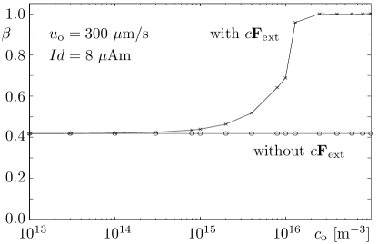
Figure 4: Fraction $\beta$ of beads caught as function of initial bead number density with and without the bulk force term $c\textbf{F}_{\text{ext}}$ in Eq. (4). The fixed values for the current-distance product $Id$ and the maximum in-flow speed $u_{\text{o}}$ are shown. At low densities less than 50% are caught; at high densities the collective motion of the beads leads to 100% capture.

Interactions and concentration. The second point we wish to make is that modification of the overall flow, and the effective bead-bead interaction this entails, is significant for bead capturing. We can study the effect by excluding momentum transfer to the fluid flow due to the bulk force term $c\textbf{F}_{\text{ext}}$ in the Navier–Stokes equation (4). At high bead number densities the force acting on the beads contributes a significant force on the fluid affecting fluid flow and spawning the effective interaction. The strength of this interaction must thus depend on the density of particles. This is illustrated in Fig. 4; capturing was simulated at fixed in-flow speed, $u_{\text{o}}=300~{}\mu$m/s, and a fixed value of the current-wire distance product, $Id=8~{}\mu$Am, but for varying bead number densities $c_{\text{o}}$ ranging from $10^{13}$ to $10^{16}$ m^-3. At low densities we find that capturing is roughly independent of density and the fraction $\beta$ of beads captured has some intermediate value, however, for high densities all beads are caught. In contrast, leaving out the bulk force term $c\textbf{F}_{\text{ext}}$ in the Navier–Stokes equation, i.e., the force acting on the fluid, gives concentration independence as shown in Fig. 4.

As can be seen in Fig. 5, a complementary way of exhibiting the importance of the bulk force term is to plot the difference $\Delta\beta=\beta_{\text{incl}}-\beta_{\text{excl}}$ between including and excluding $c\textbf{F}_{\text{ext}}$ as a function of concentration and the current-distance product. This shows that interactions makes an appreciable difference at high concentrations and intermediate magnetic fields.

Diffusion constant. Even for the small beads of radius $a=1~{}\mu$m, the diffusion constant given by the Einstein relation is small compared to the dimensions entering the problem. The time-scale for a bead to diffuse across the channel is $\tau_{\text{diff}}\sim h^{2}/D$. If we are to see the influence of diffusion competing with bead advection, then the relevant quantity is the Péclet number $hu/D$ which is advection time-scale $\tau_{\text{adv}}\sim h/u$ over the diffusion time-scale. When this number is larger than unity, which it is except for artificially large diffusion constants, then convection dominates. In the simulations the diffusion constant is increased artificially up to $10^{-11}$ m²/s in order to help numerical convergence. But we have verified that values smaller than $10^{-10}$ m²/s have no influence on the results.

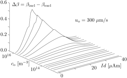
Figure 5: The difference $\Delta\beta=\beta_{\text{incl}}-\beta_{\text{excl}}$ in captured bead fractions between two situations: including and excluding the bulk force term $c\textbf{F}_{\text{ext}}$ in the Navier–Stokes equation (4). At high concentrations ($c_{\text{o}}>10^{15}$ m^-3) there is an appreciable difference between including and excluding the bulk force term, corresponding to hydrodynamic bead-bead interactions.

IV Discussion and conclusion

We have studied microfluidic capture of paramagnetic beads in suspension. The three main findings of work are: the approximate scaling shown in Fig. 3, the existence of a critical bead density for capture shown in Fig. 4, and the qualitative difference for capturing between models with and without the hydrodynamic bead-bead interaction shown in Figs. 4 and 5.

Clearly, it is very important for the capture process to include the action of the beads on the host fluid medium. Simply leaving it out can give qualitatively wrong results for high concentrations of beads. This casts some doubt on the measurement of cell susceptibility through capturing as it depends on cell concentration Zborowski et al. (2003); McCloskey et al. (2003). Deduction of susceptibilities from single bead or cell considerations together with measurements at high bead or cell concentration is suspect. Care must be taken to compare with standards of known and similar susceptibility, size, and concentration.

The effective bead-bead interaction greatly helps capturing. It should make detectable differences depending on whether there are a few or hundreds of particles in a channel at a time in actual experiments especially when the flow and magnetic field are such that the beads are barely caught one by one. This interaction should be considered when choosing operating conditions for microfluidic devices based on capturing of beads as higher bead number densities potentially eases requirements for external magnets and allows faster flushing. We hope that experimental studies will be initiated to verify this prediction of our work.

Acknowledgements. We thank Mikkel Fougt Hansen and Kristian Smistrup for valuable discussions on magnetophoresis in general and of their experiments in particular.

References

- Choi et al. (2003) J.-W. Choi, C. H. Ahn, S. Bhansali, H. T. Henderson, Sens. Actuators B 68, 34–39 (2000).
-
Pankhurst et al. (2003)
Q. A. Pankhurst,
J. Connolly,
S. K. Jones,
J. Dobson,
J. Phys. D 36, R167–181 (2003). - Zborowski et al. (2003) M. Zborowski, C. B. Fuh, R. Green, L. Sun, J. J. Chalmers, Anal. Chem. 67, 3702–3712 (1995).
-
McCloskey et al. (2003)
K. E. McCloskey,
J. J. Chalmers,
M. Zborowski,
Anal. Chem. 75, 6868–6874 (2003). - Warnke (2003) K. C. Warnke, IEEE Trans. Magn. 39, 1771–1777 (2003).
-
Mikkelsen et al. (2005)
C. Mikkelsen,
M. F. Hansen,
H. Bruus,
J. Magn. Magn. Mat. (in press, 2005). - (7) By Newton’s second law and , a spherical bead with radius approaches terminal velocity exponentially with a time constant , where is the fluid viscosity. In this work s.
- Probstein (1994) R. F. Probstein, Physicochemical hydrodynamics, an introduction (John Wiley and Sons, New York, 1994).
- (9) FEMLAB version 3.1 (COMSOL AB, Stockholm, 2004).