Light propagation in finite and infinite photonic crystals: The recursive Green’s function technique.

Abstract

We report a new computational method based on the recursive Green’s function technique for calculation of light propagation in photonic crystal structures. The advantage of this method in comparison to the conventional finite-difference time domain (FDTD) technique is that it computes Green’s function of the photonic structure recursively by adding slice by slice on the basis of Dyson’s equation. This eliminates the need for storage of the wave function in the whole structure, which obviously strongly relaxes the memory requirements and enhances the computational speed. The second advantage of this method is that it can easily account for the infinite extension of the structure both into air and into the space occupied by the photonic crystal by making use of the so-called “surface Green’s functions”. This eliminates the spurious solutions (often present in the conventional FDTD methods) related to e.g. waves reflected from the boundaries defining the computational domain. The developed method has been applied to study scattering and propagation of the electromagnetic waves in the photonic band-gap structures including cavities and waveguides. A particular attention has been paid to surface modes residing on a termination of a semi-infinite photonic crystal. We demonstrate that coupling of the surface states with incoming radiation may result in enhanced intensity of an electromagnetic field on the surface and very high $Q$ factor of the surface state. This effect can be employed as an operational principle for surface-mode lasers and sensors.

I
Introduction

Optical microcavities and photonic crystals (PC) have received increased attention in recent years because of the promising prospects of applications in a future generation of optical communication networks JP ; Sakoda . Examples of successfully demonstrated devices include lasers, light emitting diodes, waveguides, add-drop filters, delay lines, and many other review .

By far the most popular method for the theoretical description of light propagation in these systems is the finite-difference time-domain method (FDTD) introduced by Yee Yee . The success of the FDTD method is due to its speed, flexibility and ease of computational storage requirements. The limitation of the FDTD technique is related to the fact that the computational domain is finite. As the result, an injected pulse experiences spurious reflections from the domain boundaries, which leads to mixing between the incoming and reflected waves. In order to overcome this limitation the so-called perfectly matched layer condition has been introduced Berenger . However, even with this technique, a sizable part of the incoming flux can still be reflected back Mekis . In many cases the separation of spurious pulses is essential for the interpretation of the results, and this separation can only be achieved by increase of a size of the computational domain Yu . This may lead to a prohibitive amount of computational work, because the stability of the FDTD algorithm requires a sufficiently small time step.

The problem of the spurious reflections from the computational domain boundaries does not arise in the methods based on the scattering matrix technique, where the incident and outgoing fields are related with the help of the scattering matrix Maystre ; Whittaker ; Li1 ; Li2 ; Q . Other approaches where the spurious reflections are avoided include e.g. a multiple multipole method MMM , and a Green’s function method Green based on the analytical expression for the Green’s function for an empty space. The main objective of the present paper is to present a novel computational approach based on the recursive Green’s function technique that can account for an infinite extension of a photonic crystal. In this technique the Green’s function of the photonic structure is calculated recursively by adding slice by slice on the basis of Dyson’s equation. In order to account for the infinite extension of the structure both into air and into the space occupied by the photonic crystal we make use of the so-called “surface Green’s functions” that propagate the electromagnetic fields into infinity. In this paper we present a method for calculation of the surface Green’s functions both for the case of a semi-infinite homogeneous dielectrics, as well as for the case of a semi-infinite periodic structure (photonic crystal). This makes it possible to apply the Green’s function technique for investigation of a variety of important structures including waveguides and cavities in infinite or semi-infinite photonic crystals, as well as to study the effect of the surface states and the coupling of waveguide Bloch modes to the external radiation. Note that the recursive Green’s function technique is widely used for quantum mechanical transport calculations Datta ; Ferry ; Sols ; Z and is proven to be unconditionally numerically stable for various discretization schemes.

The article is organized as follows. In Section II we present a general formulation of the problem. A description of the recursive Green’s function technique is given in Section III. This section also provides a recipe for the calculation of Bloch states in a periodic structure as well as the surface Green’s function. Technical details of the calculations are given in Appendices A-C. Several examples of the application of the developed method are given in Section IV. The conclusions are presented in Section V.

II General formulation of the problem

We start with Maxwell’s equations in two dimensions

$$\frac{1}{\varepsilon_{r}(\mathbf{r})}\mathbf{\nabla}\times\left\{\mathbf{\nabla\times E(r})\right\} =\frac{\omega^{2}}{c^{2}}\mathbf{E}(\mathbf{r})$$ (1)

$$\mathbf{\nabla}\times\left\{\frac{1}{\varepsilon_{r}(\mathbf{r})}\mathbf{\nabla\times H}(\mathbf{r})\right\} =\frac{\omega^{2}}{c^{2}}\mathbf{H}(\mathbf{r}),$$

where $\mathbf{r}=x\mathbf{i}+y\mathbf{j}$, $\mathbf{\nabla}=\frac{\partial}{\partial x}\mathbf{i}+\frac{\partial}{\partial y}\mathbf{j}$, $\varepsilon_{r}(\mathbf{r})$ is the relative dielectric constant, and the electric and magnetic field vectors $\mathbf{E(r},t)=\mathbf{E(r})\exp(-i\omega t),\ \mathbf{H(r},t)=\mathbf{H(r})\exp(-i\omega t)$. If the dielectric constant $\varepsilon_{r}(\mathbf{r})$ is independent on $z$, the Maxwell’s equations decouple in two sets of equations for the TE modes ($H_{z},E_{x},E_{y}$),

$$\frac{\partial}{\partial x}\frac{1}{\varepsilon_{r}}\frac{\partial}{\partial x}H_{z}+\frac{\partial}{\partial y}\frac{1}{\varepsilon_{r}}\frac{\partial}{\partial y}H_{z}+\frac{\omega^{2}}{c^{2}}H_{z}=0,$$ (2)

$$E_{x}=\frac{i}{\omega\varepsilon_{0}\varepsilon_{r}}\frac{\partial H_{z}}{\partial y},$$

$$E_{y}=\frac{-i}{\omega\varepsilon_{0}\varepsilon_{r}}\frac{\partial H_{z}}{\partial x},$$

and for the TM modes ($E_{z},H_{x},H_{y}$),

$$\frac{1}{\varepsilon_{r}}\left(\frac{\partial^{2}E_{z}}{\partial x^{2}}+\frac{\partial^{2}E_{z}}{\partial y^{2}}\right)+\frac{\omega^{2}}{c^{2}}E_{z}=0,$$ (3)

$$H_{x}=\frac{-i}{\omega\mu_{0}}\frac{\partial E_{z}}{\partial y},$$

$$H_{y}=\frac{i}{\omega\mu_{0}}\frac{\partial E_{z}}{\partial x}.$$

Let us rewrite the equations for $H_{z},E_{z}$  (2), (3) in an operator form Sakoda

$$\mathbf{L}f=\left(\frac{\omega}{c}\right)^{2}f$$ (4)

where the Hermitian differential operator $\mathbf{L}$ and the function $f$ reads,

TE modes $$\text{:}\text{ }f\equiv H_{z},\ \mathbf{L}_{TE}=-\frac{\partial}{\partial x}\frac{1}{\varepsilon_{r}}\frac{\partial}{\partial x}-\frac{\partial}{\partial y}\frac{1}{\varepsilon_{r}}\frac{\partial}{\partial y},$$ (5)

TM modes $$\text{:}\text{ }f=\sqrt{\varepsilon_{r}}E_{z},\;\mathbf{L}_{TM}=-\frac{1}{\sqrt{\varepsilon_{r}}}\left(\frac{\partial^{2}}{\partial x^{2}}+\frac{\partial^{2}}{\partial y^{2}}\right)\frac{1}{\sqrt{\varepsilon_{r}}}$$ (6)

For the numerical solution, Eqs. (4)-(6) have to be discretized, $x,y\rightarrow m\Delta,n\Delta,$ where $\Delta$ is the grid step. Using the following discretization of the differential operators in Eqs. (5),(6) num_rec ,

$$\Delta^{2}\frac{\partial}{\partial x}\xi(x)\frac{\partial f(x)}{\partial x} \rightarrow\xi_{m+{\frac{1}{2}}}\left(f_{m+1}-f_{m}\right)-\xi_{m-{\frac{1}{2}}}\left(f_{m}-f_{m-1}\right)$$

$$\Delta^{2}\frac{\partial^{2}}{\partial x^{2}}\xi(x)f(x) \rightarrow\xi_{m+1}f_{m+1}-2\xi_{m}f_{m}+\xi_{m-1}f_{m-1}$$ (7)

we arrive to the finite difference equation

$$v_{m,n}f_{m,n}-u_{m,m+1;n,n}f_{m+1,n}-u_{m,m-1;n,n}f_{m-1,n}-$$ (8)

$$- u_{m,m;n,n+1}f_{m,n+1}-u_{m,m;n,n-1}f_{m,n-1}=\left(\frac{\omega\Delta}{c}\right)^{2}f_{m,n},$$

where the coefficients $v,u$ are defined for the cases of TE and TM modes as follows

TE modes $$\text{: }f_{m,n}=H_{z\,m,n};\;\xi_{m,n}=\frac{1}{\varepsilon_{r\,m,n}},$$ (9)

$$v_{m,n} =\xi_{m+{\frac{1}{2}},n}+\xi_{m-{\frac{1}{2}},n}+\xi_{m,n+{\frac{1}{2}}}+\xi_{m,n-{\frac{1}{2}}},$$

$$u_{m,m+1;n,n} =\xi_{m+{\frac{1}{2}},n},\;u_{m,m-1;n,n}=\xi_{m-{\frac{1}{2}},n},$$

$$u_{m,m;n,n+1} =\xi_{m,n+{\frac{1}{2}}},\;u_{m,m;n,n-1}=\xi_{m,n-{\frac{1}{2}}};$$

TM modes $$\text{:}f_{m,n}=\sqrt{\varepsilon_{r\,m,n}}E_{z\,m,n};\;\xi_{m,n}=\frac{1}{\sqrt{\varepsilon_{r\,m,n}}}$$ (10)

$$v_{m,n} =4\xi_{m,n}^{2},$$

$$u_{m,m+1;nn} =\xi_{m,n}\xi_{m+1,n},\;u_{m,m-1;nn}=\xi_{m-1,n}\xi_{m,n},$$

$$u_{m,m;n,n+1} =\xi_{m,n+1}\xi_{m,n},\;u_{m,m;n,n-1}=\xi_{m,n}\xi_{m,n-1}.$$

A convenient and common way to describe finite-difference equations on a numerical grid (lattice) is to introduce the corresponding tight-binding operator. For this purpose we first introduce creation and annihilation operators, $a_{m,n}^{+}$, $a_{m,n}.$ Let the state $|0\rangle\equiv|0,\ldots,0_{m,n},\ldots,0\rangle$ describe an empty lattice, and the state $|0,\ldots 0,1_{m,n},0,\ldots,0\rangle$ describe an excitation at the site $m,n$. The operators $a_{m,n}^{+}$, $a_{m,n}$ act on these states according to the rules Ferry

$$a_{m,n}^{+}|0\rangle=|0,\ldots 0,1_{m,n},0,\ldots,0\rangle,$$ (11)

$$a_{m,n}^{+}|0,\ldots 0,1_{m,n},0,\ldots,0\rangle=0,$$

and

$$a_{m,n}|0\rangle=0,$$ (12)

$$a_{m,n}|0,\ldots 0,1_{m,n},0,\ldots,0\rangle=|0\rangle.$$

and they obey the following commutational relations

$$[a_{m,n},a_{m,n}^{+}] =a_{m,n}a_{m,n}^{+}-a_{m,n}^{+}a_{m,n}=\delta_{m,n};$$ (13)

$$[a_{m,n},a_{m,n}] =[a_{m,n}^{+},a_{m,n}^{+}]=0.$$

Consider an operator equation

$$\widehat{\mathcal{L\,}}|f\rangle=\left(\frac{\omega\Delta}{c}\right)^{2}|f\rangle,$$ (14)

where the Hermitian operator

$$~{}\widehat{\mathcal{L}} =\sum_{m,n}(v_{m,n}a_{m,n}^{+}a_{m,n}-$$ (15)

$$-u_{m,m+1;n,n}a_{m,n}^{+}a_{m+1,n}-u_{m+1,m;n,n}a_{m+1,n}^{+}a_{m,n}-$$

$$-u_{m,m;n,n+1}a_{m,n}^{+}a_{m,n+1}-u_{m,m;n+1,n}a_{m,n+1}^{+}a_{m,n})$$

acts on the state

$$|f\rangle=\sum_{m,n}f_{m,n}a_{m,n}^{+}|0\rangle.$$ (16)

Substituting the above expressions for $\widehat{\mathcal{L}}$ and $|f\rangle$ in Eq. (14), and using the commutation relations and the rules Eqs. (11)-(13), it is straightforward to demonstrate that the operator equation (14) is equivalent to the finite difference equation (8). Note an apparent physical meaning of the last four terms in Eq. (15): terms 2 and 3 describe forward and backward hopping between two neighboring sites in the $x$-direction, and terms 4 and 5 denote similar hopping in the $y$-direction. In the next section we outline the Green’s function formalism for solution of Eq. (14).

III The recursive Green’s function technique

III.1 Basics

Let us first specify structures under investigation. We consider light propagation through a photonic structure defined in a waveguide (supercell) of the width $N,$ where we assume the cyclic boundary condition (i.e. the row $n=N+1$ coincides with the row $n=1$). The photonic structure occupies a finite internal region consisting of $M$ slices ($1\leq m\leq M$).

The external regions are semi-infinite waveguides (supercells) extending into regions $m\leq 0$ and $m\geq M+1$. The waveguides can represent air (or a material with a constant refractive index), or a periodic photonic crystal. Figure 1 shows two representative examples where (a) the semi-infinite waveguides represent a periodic photonic crystal with the period $\mathcal{M}$, and (b) a photonic structure is defined at the boundary between air and the semi-infinite photonic crystal.

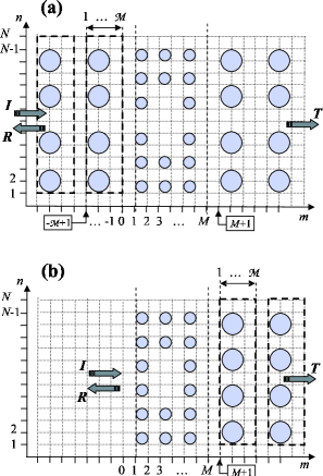
Figure 1: Schematic illustration of the system under study defined in a waveguide (supercell) of the width N. An internal region of the structure occupies M slices. Two representative cases are shown, (a) external regions are semi-periodic photonic crystals with the period $\mathcal{M}$, (b) external regions represent a semi-infinite periodic photonic crystal with the period $\mathcal{M}$ to the right and air to the left. Arrows indicate the directions on the incoming (I), reflected (R), and transmitted (T) waves.

Let us first define the scattering states for the structures under consideration. The translation invariance along the supercell dictates the Bloch form for the $\alpha$th incoming state $|\psi_{\alpha}^{\mathrm{i}}\rangle$,

$$|\psi_{\alpha}^{\mathrm{i}}\rangle=\sum_{m\leqq 0}e^{ik_{\alpha}^{+}m}\sum_{n=1}^{N}\phi_{m,n}^{\alpha}\,a_{m,n}^{+}|0\rangle,$$ (17)

where $k_{\alpha}^{+}\,(k_{\alpha}^{-})$ is the Bloch wave vector of the right-propagating (left-propagating) state $\alpha$, and $\phi_{m,n}^{\alpha}$is the corresponding Bloch transverse eigenfunction satisfying the Bloch condition

$$\phi_{m,n}^{\alpha}=\phi_{m+\mathcal{M},n}^{\alpha}.$$ (18)

The transmitted and reflected states, $|\psi_{\alpha}^{\mathrm{t}}\rangle$ and $|\psi_{\alpha}^{\mathrm{r}}\rangle$, can be written in a similar form,

$$|\psi_{\alpha}^{\mathrm{t}}\rangle =\sum_{m\geqq M+1}\sum_{\beta}t_{\beta\alpha}e^{ik_{\beta}^{+}(m-(M+1))}\sum_{n=1}^{N}\phi_{m,n}^{\beta}\,a_{m,n}^{+}|0\rangle,$$ (19)

$$|\psi_{\alpha}^{\mathrm{r}}\rangle =\sum_{m\leqq 0}\sum_{\beta}r_{\beta\alpha}e^{ik_{\beta}^{-}m}\sum_{n=1}^{N}\phi_{m,n}^{\beta}\,a_{m,n}^{+}|0\rangle,$$ (20)

where $t_{\beta\alpha}\,(r_{\beta\alpha})$ stands for the transmission (reflection) amplitude from the incoming Bloch state $\alpha$ to the transmitted (reflected) Bloch state $\beta.$ Note that in general case the wave vectors $k_{\alpha}^{\pm}$ and the Bloch states $\phi_{m,n}^{\alpha}$ can be different in the left and right waveguides (see e.g. Fig. 1(a), when the photonic structure is defined at the boundary air/photonic crystal). The method of calculation of the Bloch states for an arbitrary periodic structure is described below in Section IIIC.

We define Green’s function of the operator $\widehat{\mathcal{L\,}}$ in a standard way,

$$\left(\left(\omega\Delta/c\right)^{2}-\widehat{\mathcal{L\,}}\right)G(\omega)=\widehat{1\mathcal{\,}},$$ (21)

where $\widehat{1\mathcal{\,}}$ is the unitary operatorEconomou . The knowledge of the Green’s function allows one to calculate the transmission and reflection coefficients. Indeed, let us write down the solution of Eq. (14) as a sum of two terms, the incoming state $|\psi^{\mathrm{i}}\rangle$ and the system response $|\psi\rangle$ representing whether the transmitted or reflected states, $|\psi^{\mathrm{t}}\rangle$ or $|\psi^{\mathrm{r}}\rangle$, $|f\rangle=|\psi^{\mathrm{i}}\rangle+|\psi\rangle.$ Substituting $|f\rangle$ into Eq. (14) and using the formal definition of the Green’s function Eq. (21), the solution of Eq. (14) can be written in the form

$$|\psi\rangle=G\left(\widehat{\mathcal{L\,}}-\left(\omega\Delta/c\right)^{2}\right)|\psi^{\mathrm{i}}\rangle.$$ (22)

Calculating the matrix elements $\langle M+1,n|\psi\rangle\equiv\langle 0|a_{M+1,n}\psi\rangle$ and $\langle 0,n|\psi\rangle\equiv\langle 0|a_{0,n}\psi\rangle,$ of the rigth and left hand side of Eq. (22), we arrive to the $N\times N$ system of linear equations for the transmission and reflection amplitudes (see for details Appendix A),

$$\Phi_{M+1}T =-G^{M+1,0}(U_{0,1}\Phi_{-\mathcal{M+}1}K_{l}-{\Gamma_{l}}^{-1}\Phi_{0})$$ (23)

$$\Phi_{0}R =-G^{0,0}(U_{0,1}\Phi_{-\mathcal{M+}1}K_{l}-{\Gamma_{l}}^{-1}\Phi_{0})-\Phi_{0}$$ (24)

where the matrix elements $(T)_{\beta\alpha}=t_{\beta\alpha},$ $(R)_{\beta\alpha}=r_{\beta\alpha};$ $G^{M+1,0}$ and $G^{0,0}$ are the Green’s function matrixes with the elements

$$(G^{m,l})_{n,p}=\langle 0|a_{m,n}G\,a_{l,p}^{+}|0\rangle.$$ (25)

$\Gamma_{l}\equiv G_{\mathrm{wg}}^{0,0}$ is the left “surface Green’s function” corresponding only to part of the whole structure, namely, to the semi-infinite waveguide (supercell) that extends to the left, $-\infty<m\leq 0.$ The physical meaning of the surface Green’s function $\Gamma$ is that it propagates the electromagnetic fields from the boundary slice of the semi-infinite waveguide (supercell) into infinity. A method for calculation of the surface Green’s functions both for the case of a semi-infinite homogeneous dielectrics, as well as for the case of a semi-infinite photonic crystal in a waveguide geometry is described below in Section IIID. The matrixes $K_{l}$ and $\Phi_{m}$ are given by the right-propagating Bloch eigenvectors $k_{\alpha}^{+}\,$and the corresponding eigenstates $\phi_{m,n}^{\alpha}$ in the waveguides,

$$(K_{l})_{\alpha\beta}=\exp(ik_{\alpha}^{+})\,\delta_{\alpha\beta};(\Phi_{m})_{n\alpha}=\phi_{m,n}^{\alpha}\;$$ (26)

and the diagonal “hopping matrix” $U_{0,1}$ is defined as

$$(U_{0,1})_{n,n^{\prime}}=u_{0,1;n,n^{\prime}}\delta_{n,n^{\prime}}.$$ (27)

(Note that the matrix $K_{l}$ in Eqs. (23),(24) refers to the right-propagating states in the left waveguide). In the following sections we describe the recursive Green’s function technique based on the successive use of the Dyson’s equation, introduce the method for the calculation of Bloch states in a periodic structure, and outline the way to calculate the surface Green’s function $\Gamma.$

III.2 Recursive technique based on Dyson’s equations

In order to calculate Green’s function of the internal structure (i.e. for the slices $1\leq m\leq M$) we utilize the recursive technique based on Dyson’s equation, see Fig. 2.

Figure 2: Schematic illustration of the application of Dyson’s equation for calculation of Green’s function for a composed structure consisting of $m$+1 slices (see text for details). The operators $\widehat{\mathcal{L\,}}_{m}^{0}$ and $\widehat{\mathit{l}\mathcal{\,}}_{m+1}^{0}$ describe respectively the structure composed of $m$ slices, and the ($m+1$)-th slice. The operator $\widehat{\mathcal{L\,}}_{m+1}=\widehat{\mathcal{L\,}}_{m}^{0}+\widehat{\mathit{l}\mathcal{\,}}_{m+1}^{0}+\widehat{\mathcal{V\,}}$ corresponds to the composed structure of $m+1$ slices, where $\widehat{\mathcal{V\,}}$ is the perturbation operator describing the hopping between the $m$th and ($m+1$)-th slices.

In order to illustrate this technique let us consider a structure consisting of $m$ slices

. The operator $\widehat{\mathcal{L\,}}_{m}^{0}$ describing this structure can be written down in the form

$$\widehat{\mathcal{L\,}}_{m}^{0}=\sum_{\mathbf{r}}v_{\mathbf{r}}a_{\mathbf{r}}^{+}a_{\mathbf{r}}-\sum_{\mathbf{r,\Delta}}u_{\mathbf{r,r+\Delta}}a_{\mathbf{r}}^{+}a_{\mathbf{r+\Delta}},$$ (28)

where $\mathbf{r}=m^{\prime},n^{\prime}\ (1\leq m^{\prime}\leq m;1\leq n^{\prime}\leq N),$ and the summation over $\Delta$ in the second term is performed over all available nearest neighbors. Suppose we know Green’s function $G_{m}^{0}$ of the operator $\widehat{\mathcal{L\,}}_{m}^{0}$, as well as Green’s function $g_{m+1}^{0}$ of the the operator $\widehat{\mathit{l}\mathcal{\,}}_{m+1}^{0}$ corresponding to a single ($m+1$)-th slice,

$$~{}\widehat{\mathit{l}\mathcal{\,}}_{m+1}^{0} =\sum_{n}(v_{m+1,m+1}a_{m+1,n}^{+}a_{m+1,n}-$$ (29)

$$-u_{m+1,m+1;n,n+1}a_{m+1,n}^{+}a_{m+1,n+1}-$$

$$-u_{m+1,m+1;n+1,n}a_{m+1,n+1}^{+}a_{m+1,n}).$$

(The method of calculation of Green’s function for a single slice is outlined in Appendix C). Our aim is to calculate Green’s function of the composed structure, $G_{m+1}$, consisting of $m+1$ slices. The operator corresponding to this structure can be written down in the form

$$\widehat{\mathcal{L\,}}_{m+1}=\widehat{\mathcal{L\,}}_{m}^{0}+\widehat{l\mathcal{\,}}_{m+1}^{0}+\widehat{\mathcal{V\,}},$$ (30)

where the operators $\widehat{\mathcal{L\,}}_{m}^{0}$ and $\widehat{l\mathcal{\,}}_{m+1}^{0}$ are given by the expressions Eqs. (30), (29), and $\widehat{\mathcal{V\,}}=$ $\widehat{\mathcal{V\,}}_{m,m+1}+$ $\widehat{\mathcal{V\,}}_{m+1,m}$ is the perturbation operator describing the hopping between the $m$th and ($m+1$)-th slices,

$$~{}\widehat{\mathcal{V\,}} =\widehat{\mathcal{V\,}}_{m+1,m}+\widehat{\mathcal{V\,}}_{m,m+1}=$$ (31)

$$=-\sum_{n}(u_{m,m+1;n,n}a_{m,n}^{+}a_{m+1,n}+$$

$$+u_{m+1,m;n,n}a_{m+1,n}^{+}a_{m,n}).$$

The Green’s function of the composed structure, $G_{m+1},$ can be calculated on the basis of Dyson’s equationEconomou

$$G_{m+1} =G^{0}+G^{0}\widehat{\mathcal{V}}G_{m+1},$$ (32)

$$G_{m+1} =G^{0}+G_{m+1}\widehat{\mathcal{V}}G^{0},$$

where $G^{0}$ is the ‘unperturbed’ Green’s function corresponding to the operators $\widehat{\mathcal{L\,}}_{m}^{0}$ or $\widehat{l\mathcal{\,}}_{m+1}^{0}$. For the sake of completeness, a brief derivation of Dyson’s equation is given in Appendix B. Thus, starting from Green’s function for the first slice $g_{1}^{0}$ and adding recursively slice by slice we are in the position to calculate Green’s function of the internal structure consisting of $M$ slices. Explicit expressions following from Eqs. (32) and used for the recursive calculations are given below,

$$G_{m+1}^{m+1,m+1} =(I-g_{m+1}^{0}U_{m+1,m}(G_{m}^{0})^{m,m}U_{m,m+1})^{-1}g_{m+1}^{0},$$

$$G_{m+1}^{m+1,1} =G_{m+1}^{m+1,m+1}U_{m+1,m}(G_{m}^{0})^{m,1},$$

$$G_{m+1}^{1,1} =(G_{m}^{0})^{1,1}+(G_{m}^{0})^{1,m}U_{m,m+1}G_{m+1}^{m+1,1},$$

$$G_{m+1}^{1,m+1} =(G_{m}^{0})^{1,m}U_{m,m+1}G_{m+1}^{m+1,m+1},$$

where the upper indexes define the matrix elements of the Green’s function $G^{m,m^{\prime}}=\langle 0|a_{m,n}G\,a_{m^{\prime},n^{\prime}}^{+}|0\rangle$. This recursive technique is proven to be unconditially numerically stable Datta ; Ferry ; Sols . The performance of the method is determined by the size of the system of linear equations (III.2) which we solve when we add each consecutive slice. This system is solved $M$ times, where $M$ is the number of slices of the internal structure (in the $x$-direction). The size of Eqs. (III.2) is $N\times N$, where $N$ is a number of discretization points in the $y$-direction. Typical dimensions of the equations used for computations of the structures reported in Section 4 are $\thicksim 200\times 200.$

In order to calculate the Green’s function of the whole system, we have to connect the internal structure with the left and right semi-infinite waveguides. Starting with the left waveguide, we write

$$\widehat{\mathcal{L\,}}_{int+left}=\widehat{\mathcal{L\,}}_{int}+\widehat{\mathcal{L\,}}_{left}+\widehat{\mathcal{V\,}},$$ (34)

where the operators $\widehat{\mathcal{L\,}}_{int+left},\widehat{\mathcal{L\,}}_{int}$ and $\widehat{\mathcal{L\,}}_{left}$ describe respectively the system representing the internal structure + the left waveguide, the internal structure, and the left waveguide. The perturbation operator $\widehat{\mathcal{V}}\mathcal{\,}$ describes the hopping between the left waveguide and the internal structure. Applying then the Dyson equation in a similar way as we described above,

$$G_{int+left}=G^{0}+G^{0}\widehat{\mathcal{V}}G_{int+left},$$ (35)

we are in the position to find the Green’s function $G_{int+left}$ of the system representing the internal structure + the left waveguide. $G^{0}$ in Eq. (35) in an ‘unperturbed’ Green’s function corresponding to the internal structure and the semi-infinite waveguide (the “surface Green’s function” $\Gamma).$ Having calculated the Green’s function $G_{int+left}$ on the basis of Eq. (35), we proceed in a similar way by adding the right waveguide and calculating with the help of the Dyson’s equation the total Green’s function $G$ of the whole system.

III.3 Bloch states of the periodic structure

In this section we describe the method for calculation of the Bloch states in periodic waveguides (supercells) using the Green’s function technique. Similar method was used for calculation of Bloch states in quantum-mechanical structuresZ .

Consider a unit cell of a periodic waveguide occupying $\mathcal{M}$ slices, $1\leq m\leq\mathcal{M}$, see Fig. 3.

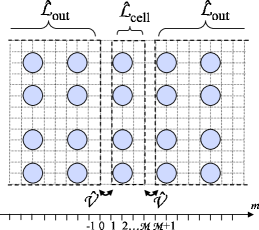
Figure 3: Schematic illustration of the calculation of Bloch states in an infinite periodic structure (see text for details). The operator $\widehat{\mathcal{L\,}}_{\mathrm{cell}}$ describes a unit cell under consideration, $1\leq m\leq\mathcal{M}$, and $\widehat{\mathcal{L\,}}_{\mathrm{out}}$ describes the rest of the structure. The hopping between the cell and the rest of the structure is described by the operator $\widehat{\mathcal{V\,}}$.

Rewrite the operator corresponding to the whole structure in the form

$$\widehat{\mathcal{L\,}}=\widehat{\mathcal{L\,}}_{\mathrm{cell}}+\widehat{\mathcal{L\,}}_{\mathrm{out}}+\widehat{\mathcal{V\,}},$$ (36)

where the operators $\widehat{\mathcal{L\,}}_{\mathrm{cell}}$ and $\widehat{\mathcal{L\,}}_{\mathrm{out}}$ describe respectively the cell under consideration ($1\leq m\leq\mathcal{M}$), and the outside region including all other slices $-\infty<m\leq 0$ and $\mathcal{M+}1\leq m<\infty$, and $\widehat{\mathcal{V\,}}$ is the hopping operator between the cell and slices $m=0$ and $m=\mathcal{M}+1$. Write the total wave function $|\psi\rangle=\sum_{m,n}\psi_{m,n}a_{m,n}^{+}|0\rangle$ in the form

$$|\psi\rangle=|\psi_{\mathrm{cell}}\rangle+|\psi_{\mathrm{out}}\rangle,$$ (37)

where $|\psi_{\mathrm{cell}}\rangle$ and $|\psi_{\mathrm{out}}\rangle$ are respectively wave functions in the cell and in the outside region. Substituting Eqs. (36),(37) into Eq. (14), we obtain $|\psi_{\mathrm{cell}}\rangle=G_{\mathrm{cell}}\widehat{\mathcal{V\,}}|\psi_{\mathrm{out}}\rangle,$ where $G_{\mathrm{cell}}$ is the Green’s function of the operator $\widehat{\mathcal{L\,}}_{\mathrm{cell}}$. Calculating the matrix elements $\langle 1,n|\psi\rangle$ and $\langle\mathcal{M},n|\psi\rangle$, this equation can be written in the matrix form,

$$\psi_{1} =G_{\mathrm{cell}}^{1,1}U_{1,0}\psi_{0}+G_{\mathrm{cell}}^{1,\mathcal{M}}U_{1,0}\psi_{\mathcal{M}+1}$$ (38a)

$$\psi_{\mathcal{M}} =G_{\mathrm{cell}}^{\mathcal{M},1}U_{1,0}\psi_{0}+G_{\mathrm{cell}}^{\mathcal{M},\mathcal{M}}U_{1,0}\psi_{\mathcal{M}+1},$$ (38b)

where the vector column $$\psi_{m}= \left(\psi_{m,1}\ldots\psi_{m,N}\right)^{T} U_{\mathcal{M},\mathcal{M}+1}=U_{0,1} U_{0,1}=U_{1,0} U$$ , and where we used (because of the periodicity) and (according to the definition of , Eq.(27)). It is convenient to rewrite Eq. (38a) in a compact form

$$T_{1}\left(\begin{array}[]{c}\psi_{\mathcal{M}+1}\\ \psi_{\mathcal{M}}\end{array}\right)=T_{2}\left(\begin{array}[]{c}\psi_{1}\\ \psi_{0}\end{array}\right),\;\mathrm{where}$$ (43)

$$T_{1}=\begin{pmatrix}-G_{\mathrm{cell}}^{1,\mathcal{M}}U_{1,0}&\;0\\ G_{\mathrm{cell}}^{\mathcal{M},\mathcal{M}}U_{1,0}&\;I\end{pmatrix},\;T_{2}=\begin{pmatrix}-I&\;-G_{\mathrm{cell}}^{1,1}U_{1,0}\\ 0&\;G_{\mathrm{cell}}^{\mathcal{M},1}U_{1,0}\end{pmatrix},$$

with $I$ being the unitary matrix. The wave function of the periodic structure has Bloch form,

$$\psi_{\mathcal{M}+m}=e^{ik_{x}\mathcal{M}}I\psi_{m}.$$ (44)

Combining Eqs. (43) and (44), we arrive to the eigenequation for Bloch wave vectors and Bloch states,

$$T_{1}^{-1}T_{2}\left(\begin{array}[]{c}\psi_{1}\\ \psi_{0}\end{array}\right)=e^{ik_{x}\mathcal{M}}\left(\begin{array}[]{c}\psi_{1}\\ \psi_{0}\end{array}\right),$$ (45)

determining the set of Bloch eigenvectors $k_{x}^{\alpha}$ and eigenfunctions $\psi^{\alpha},$ $1\leq\alpha\leq N.$

To improve numerical stability of Eq. (45), it may be rewritten in the form Li2 :

$$(T_{1}+T_{2})^{-1}T_{1}\left(\begin{array}[]{c}\psi_{1}\\ \psi_{0}\end{array}\right)=(e^{ik_{x}\mathcal{M}}+1)^{-1}\left(\begin{array}[]{c}\psi_{1}\\ \psi_{0}\end{array}\right).$$ (46)

This technique allows one to avoid overflows and underflows in the eigensolver routine when eigenvalues with $|e^{ik_{x}\mathcal{M}}|\gg 1$ and $|e^{ik_{x}\mathcal{M}}|\ll 1$ are calculated.

In order to separate the left- and right-propagating states we compute the Poynting vector integrated over transverse direction, whose sign determines the direction of propagation. Bloch state propagating in a waveguide (supercell) defined in a photonic crystal is illustrated below in Fig. 5(c).

Poynting vector can be expressed as follows Sakoda

$$\mathbf{S}_{\alpha}(y)=\frac{1}{2}\Re[\mathbf{E}_{\alpha}(y)\times\mathbf{H}_{\alpha}^{\ast}(y)].$$ (47)

Note that for the case of the waveguide defined in air, $\mathcal{M}=1$, and Green’s functions $G_{\mathrm{cell}}$ in Eq. (43) is simply given by Green’s function of a single slice $g^{0}$ (see Appendix C for details of calculation of $g^{0}$).

III.4 The surface Green’s function $\Gamma.$

Consider a semi-infinite Bloch waveguide (supercell) of the periodicity $\mathcal{M}$ extending in the region $-M\leq m<\infty$ as depicted in Fig. 4

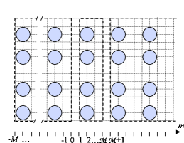
Figure 4: A schematic diagram illustrating calculation of the surface Green’s function $\Gamma$ of a periodic structure (see text for details).

Suppose that an excitation $|s\rangle$ is applied to its first slice $m=-M$. Introducing the Green function $G_{\mathrm{wg}}$ corresponding to the operator $\widehat{\mathcal{L\,}}_{\mathrm{wg}}$ describing the waveguide, one can write down the response to the excitation $|s\rangle$ in the form

$$|\psi\rangle=G_{\mathrm{wg}}|s\rangle,$$ (48)

where $|\psi\rangle$ is the wave function that has to satisfy Bloch conditions (44). Applying Dyson’s equation between the slices $0$ and $1$ we obtain

$$G_{\mathrm{wg}}^{1,-M}=\Gamma_{r}U_{1,0}G_{\mathrm{wg}}^{0,-M},$$ (49)

where $\Gamma_{r}\equiv G_{\mathrm{wg}}^{1,1}$ is the right surface Green’s function. (Note that because the waveguide is infinitely long and periodic, $G_{\mathrm{wg}}^{1,1}=G_{\mathrm{wg}}^{\mathcal{M}+1,\mathcal{M}+1}=G_{\mathrm{wg}}^{2\mathcal{M}+1,2\mathcal{M}+1}=$ … etc.). Taking the matrix elements $\langle 1,n|\psi\rangle$ of Eq. (48) and making use of Eq. (49), we obtain for an each Bloch state $\alpha$, $\psi_{1}^{\alpha}=$ $\Gamma_{r}U_{1,0}\psi_{0}^{\alpha}.$ The latter equation can be used for determination of $\Gamma_{r}$,

$$\Gamma_{r}U_{1,0}=\Psi_{1}\Psi_{0}^{-1},$$ (50)

where $\Psi_{1}$ and $\Psi_{0}$ are the square matrixes composed of matrix-columns $\psi_{1}^{\alpha}$ and $\psi_{0}^{\alpha},$ Eq. (45). If the waveguide is open to the left, its surface Green’s function is the same as the surface Green’s function of the corresponding waveguide open to the right, $\Gamma_{l}=\Gamma_{r}.$ Note that for the case of the waveguide defined in air the surface Green’s function (50) simplifies to $\Gamma_{r}U_{1,0}=K$, where $K$ is defined according to Eq. (26).

IV Applications of the method

To reveal the power of the method we study three model systems defined in 2D square-lattice photonic crystal. First, we calculate a transmission coefficient and quality factor ($Q$ factor) of several representative types of microcavities in infinite PCs. Then we focus on semi-infinite crystals where we investigate the effect of surface states, and, finally, we consider a semi-infinite PC with a waveguide opening to the surface. For the bulk crystal we choose a structure composed of cylindrical rods with the permittivity $\varepsilon_{r}=8.9$ and the diameter of a rod $d=0.4a$ in a vacuum background, where $a$ is the size of the unit cell. Each unit cell is discretized into 25 points in both $x$ and $y$ directions.

Most of photonic crystal devices operate in a bandgap. The structure at hand has a complete bandgap for TM-modes in the frequency range $0.32\lesssim\omega a/2\pi c\lesssim 0.44$ JP , and does not have a complete bandgap for the TE-polarization. Because of this, we will hereafter consider the TM-modes only.

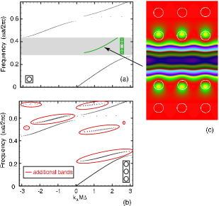
Figure 5: (color online) (a) Band diagram for the right-propagating TM-mode of an infinite 2D photonic crystal ($\varepsilon_{r}=8.9$, $d=0.4a$) in $\Gamma X$-direction. PC has a fundamental bandgap in the frequency range $0.28\lesssim\omega a/2\pi C\lesssim 0.44$ (filled with gray in the figure). Green line in the fundamental bandgap corresponds a guided mode in a waveguide created by removing a central row of rods from the PC as shown in the inset. (b) Additional bands (encircled with red) originated from the finite size effect. The waveguide (supercell) contains three unit cells in the transverse direction as illustrated in the inset. (c) Bloch state propagating in the PC waveguide at $\omega a/2\pi c=0.38$

The developed method allows one to treat structures unlimited in $x$-direction, whereas in $y$-direction the structure of interest is confined within a supercell with imposed cyclic boundary conditions. This leads to the finite size effects in a photonic band structure. If the supercell consists more than one elementary cell, additional bands appear along with the bands for infinite PC (Fig. 5 (a,b)), as the result of the imposed boundary conditions in the transverse direction.

A similar finite size effect emerges when air waveguides (supercells) are attached to the system of interest. Even though we send a wave from an open space, we use a finite number of propagating modes. Solution of the eigenvalue problem (4) for the air supercell gives a discrete set of right-propagating eigenstates $k_{x}^{m}=\sqrt{\omega^{2}/c^{2}-(2\pi m/w)^{2}}$ where $w$ is the width of the supercell, and $m$ is integer such that $\max{|m|}<\omega w/2\pi c$. Thus, a wave incident from air effectively propagates only at certain incidence angles, determined by the ratio of the longitudinal and transverse wave vectors $\tan\alpha=k_{y}^{m}/k_{x}^{m}$, as illustrated in Fig. 6. Note that this finite size effect (caused by the cyclic boundary conditions in the $y$-direction) might in some cases represent a drawback of the method.

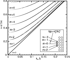
Figure 6: Dispersion relation for the air supercell of the width of 9$a$. Effective angles of incidence are determined by the angular wavenumber $m$. Inset shows the effective angles of incidence for $m=-2,-1,0,1,2$.

IV.1 Microcavity

In this section we consider a microcavity defined in a waveguide in an infinite PC. The waveguide is created by removing a single central row of cylinders, such that in the energy range corresponding the fundamental bandgap only one waveguide mode can propagate. Band diagram of the waveguide mode is shown in Fig.5 (a).

Three different cavities are introduced in order to show the effect of geometry and demonstrate the importance of proper design of a cavity. The first cavity is defined by two rods placed on the lattice sites, see insets in Fig.7. In the second structure the diameter of the rods is doubled, and for the third cavity we place two rods from each side of the cavity to achieve better confinement. A dependence of the transmission coefficient on the incoming wave frequency is depicted in Fig.7(a). We would like to stress that in the calculation of the transmission coefficient, the incoming, transmitted and reflected states are the Bloch states of a waveguide (shown in Fig.5(c)), such that all spurious reflections from PC interfaces or computational domain boundaries are avoided.

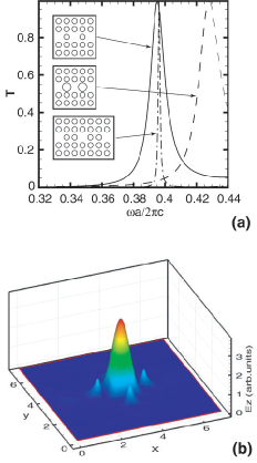
Figure 7: (color online) (a) Transmission coefficient of three cavity structures versus frequency. (b) Intensity of the $E_{z}$-component of the electromagnetic field in the double-wall cavity at the resonance ($\omega a/2\pi c=0.3952$).

The fundamental parameter of cavity resonances is their $Q$-factor defined as $Q$=2$\pi\omega$*(stored energy)/(energy lost per cycle), which can be rewritten in the following form:

$$Q=\omega\frac{\Omega}{4\int S_{in}dy}$$

where $\Omega_{TM}=\int[\varepsilon\varepsilon_{0}|E_{z}|^{2}+\mu_{0}(|H_{x}|^{2}+|H_{y}|^{2})]dxdy$  and $\Omega_{TE}=\int[\mu_{0}|H_{z}|^{2}+\varepsilon\varepsilon_{0}(|E_{x}|^{2}+|E_{y}|^{2})]dxdy$ characterizes the energy stored in the system respectively for TM and TE polarizations and the integral over $S_{in}$ is the incoming energy flux. Eq. (IV.1) can be also expressed as a well-known relation $Q=\omega/\Delta\omega$ where $\omega$ is the resonant frequency and $\Delta\omega$ is the width of the resonant peak at half-maximum.

The resonance peak for the single-wall cavity is centered at $\omega a/2\pi c=0.3952$ and has $Q$ factor 35.5. As expected, the highest $Q$ factor (327.7) is achieved for the case of double-rod walls. Resonance peak in the case of larger rods is shifted to the higher energy values ($\omega a/2\pi c=0.4281$) because of the decrease of the effective size of the cavity. The lower $Q$ factor in this case (25.07) is because the larger rods disrupt destructive interference in a bandgap of the PC.

Note that the width of the supercell used in the computations has to be large enough to ensure that the intensity of the field decays to zero at the domain boundaries. At the same time, it is desirable to have the size of the computational domain as small as possible. For the present computations, keeping this trade-off in mind, we have chosen a supercell consisting of 7 unit cells in the $y$-direction. This choice seems to be sufficient, as the field intensity decreases by 5 orders of magnitude within the length of two lattice constants from the waveguide towards the supercell boundaries.

Finally, to confirm our results and to verify the developed method, we performed calculations for the cavities and waveguides in PC studied by Li et al.Li2 and found a full agreement with their results.

IV.2 Surface states

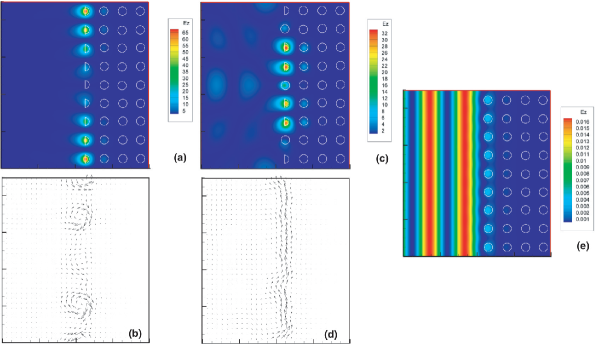
Figure 8: (color online) $E_{z}$ field and Poynting vector distributions for the structure 1 ((a),(b)) and for the structure 2 ((c),(d)) at the resonant frequencies (marked by arrows in Fig. 9). (e) $E_{z}$ field distributions for the structure that does not support surface modes (a semi-infinite photonic crystal with all identical cylindrical rods). In all cases the structures are illuminated by the incoming wave with the incidence angle $\alpha=\arctan{k_{y}/k_{x}=34.7}^{\circ}$.

In the previous section we considered wave propagation in an infinite photonic crystal. Another aspect of interest is the effect of the surface in semi-infinite photonic crystals that can accommodate a localized state (surface mode) decaying both into air and into a space occupied by the photonic crystalJP ; Elson_OPTE_2004 . In the present section we study the coupling between an incident radiation and the surface states. Note that a surface mode residing on the surface of an infinite (in the $y$-direction) photonic crystal represents a truly bound state with the infinite lifetime. However, because of the used cyclic boundary conditions, our system is effectively confined in the transverse direction. As the result, the translation symmetry is broken, and the surface mode turns into a resonant state with a finite lifetime. Using the developed method, we calculate the $Q$ factor of the surface modes. Our findings indicate that the surface modes, thanks to their high $Q$ factors, can be used for lasing and sensing applications.

We study two semi-infinite photonic crystal structures that support localized surface modes. In the first case a surface row of cylinders is composed of half-truncated rodsJP (structure 1), and in the second case the cylindrical and half-truncated rods in the surface row are interchanged as shown in Fig. 8 (structure 2). In order to calculate the $Q$ factor of the structures at hand, we illuminate the semi-infinite photonic crystal by an incidence wave (that excites the surface modes) and compute the intensity of the field distribution. Note that the calculated field distribution includes the contributions from both the surface mode exited by the incident light, as well as the incident and reflected waves. This leads to a nearly constant off-resonance background in the dependence $Q=Q(\omega)$ that is caused by the contribution of the incident and reflected waves in the total field intensity in Eq. (IV.1). To remove this background we calculate the $Q$ factor of a structure without surface states. We choose this structure as a semi-infinite photonic crystal with all identical cylindrical rods, which is known not to support surface modes JP . Then the obtained value is subtracted from the calculated value of the $Q$ factor of the system under study. Note that in the calculation of the $Q$ factor, the surface integration in Eq. (IV.1) is performed over the area depicted in Fig. 8.

Figure 9 shows a $Q$ factor of structures 1 and 2 as a function of the frequency of the illuminating light. For both structures the $Q$ factor reaches $\sim 10^{4}$. Figures 8 (a),(c) show $E_{z}$-field distribution for structures 1 and 2 at the resonance. For a comparison, a field distribution for a structure that does not support a surface mode (a semi-infinite photonic crystal with all identical cylindrical rods) is shown in Figure 8 (e). In the latter case the field intensity rapidly decays into the bulk of the photonic crystal, whereas for the structures supporting the surface modes, the intensity is strongly localized at the boundary row of rods. It is also worth to mention that for the latter case the intensity of the field in the surface mode exceeds the incoming light intensity by 4 orders of magnitude, such that the light intensity in the air region is not visible in the figures (compare 8 (a),(c) with (e)).

One can easily estimate the position of the resonant frequency for the surface modes. Indeed, the outermost row of the cylinders (where the surface state resides) can be considered as a resonator with the characteristic resonant wavelengths following from the cyclic boundary conditions and given by $\lambda_{\alpha}=2\pi/k_{\alpha}$, where

$$k_{\alpha}=\frac{2\pi\alpha}{w},$$ (51)

$\alpha$ is the mode number and $w$ is the width of the waveguide. The surface state for structure 1 exists only in a limited frequency interval, $0.33\lesssim\omega a/2\pi c\lesssim 0.37$ (the dispersion relation of the surface mode of this structure is given in Ref. JP, ). It follows from this dispersion relation that all the modes given by Eq. (51), except $\alpha=4,$ are situated outside this interval, whereas the mode $\alpha=4$ corresponds to the frequency $\omega a/2\pi c=0.365$. This estimated frequency agrees very well with the actual calculated resonant frequency $\omega a/2\pi c\approx 0.359$, see Fig. 9. Note that the calculated field distribution, Fig. 8 (a), is fully consistent with the expected pattern for 4th mode in the system of $n=9$ cylinders. (This field distribution is determined by the overlap of the eigenstate corresponding to the eigenfrequency (51) with the actual positions of the cylinders in the outermost row). Note that we performed calculations for different numbers of cylinders in the transverse directions ($n=5,...,11$), and we always find an excellent agreement with the predicted value of the resonant frequency $\omega_{\alpha}.$

Figures 8 (b),(d) show Poynting vector distribution for both structures at the resonance. For the structure 1 the Poynting vector is “curling” along the boundary, showing a low speed of the surface state. In contrast, for the structure 2, the Poynting vector exhibits a rapid flow of energy along the boundary. Another difference between these structures is a very broad and rather strong “background” peak in the structure 2 in the region $0.34\lesssim\omega a/2\pi c\lesssim 0.35$ (with $Q$ factor up to $\sim 100$). The presence of such the peak indicates that the corresponding surface state can be rather robust to various kinds of imperfections that are always present in real structures and which are known to broaden the resonances and lead to decrease of the $Q$ factor Q . These two examples of photonic crystals illustrate, that with proper structure design one can engineer and tailor properties of the surface states into the required needs.

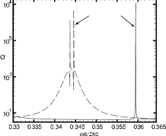
Figure 9: Dependencies $Q=Q(\omega)$ for structures 1 and 2 (solid and dashed lines respectively). Arrows indicate the resonances for which the field intensities and Poynting vectors are visualized in Fig. 8

High values of the $Q$ factors of the surface modes residing at the interface of the photonic crystal structures indicate that these systems can be used for lasing and sensing applications. The lasing effect has been demonstrated for different photonic crystal structures including band-gap defect mode lasersdefect_mode , distributed feedback lasers feedback , and bandedge lasersbandedge . Utilization of the high-Q factor of the surface modes represent a novel way to sustain lasing emission. To achieve lasing effect careful design of the surface and surface mode engineering should be performed and the developed method seems to be a suitable tool for this purpose. A detailed study of the surface modes for various surface terminations, their $Q$-values, and dispersion relations will be reported elsewhere.

IV.3 Waveguide coupled to the open space

The last example of application of the method presented here is a semi-infinite photonic crystal with a waveguide coupled to the surface, see Fig. 10. It has been recently demonstrated that a surface of a photonic crystal can serve as a kind of antenna to beam the light emitted from the waveguide in a single directionKramper_PRL_2004 ; Moreno_PRB_2004 . These findings outline the importance of investigation of the surface modes in the photonic band-gap structures that can eventually open up the possibilities to integrate such the devices with conventional fiber optic devices.

In the present section we consider two different crystal terminations to illustrate the effect of the surface on propagation of the light emitted from the waveguide. In the first case the surface is composed of cylinders with parameters identical to those in the bulk of the crystal, and in the second case the surface cylinders are two times smaller than the cylinders in the bulk.

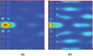
Figure 10: (color online) $E_{z}$ field distributions at the surface of a truncated photonic crystal with a waveguide. (a) The surface is composed of cylinders with parameters identical to those in the bulk of the crystal, and (b) the surface cylinders are two times smaller than the cylinders in the bulk.

The Bloch state propagating in a waveguide in the photonic crystal couples with the states in air and the resulting field distributions is shown in Fig. 10. The first structure does not support the surface mode, and hence the light intensity distribution in the air region exhibits a typical diffraction pattern. However, for the case of the second structure the field distribution in the air region is drastically different. In this case the Bloch state in the waveguide couples with the surface state localized at the crystal termination, such that the whole surface acts as a source of radiation.

V Conclusions

We have developed a method based on the recursive Green’s function technique for the numerical study of photonic crystal structures. The method is proven to be an effective and numerically stable tool for design and simulation of both infinite photonic crystals and photonic crystals with boundaries. In the present method the Green’s function of the photonic structure is calculated recursively by adding slice by slice on the basis of Dyson’s equation. In order to account for the infinite extension of the structure both into air and into the space occupied by the photonic crystal we make use of the so-called “surface Green’s functions” that propagate the electromagnetic fields into infinity. This eliminates the spurious solutions (often present in the conventional FDTD methods) related to e.g. waves reflected from the boundaries defining the computational domain. The developed method has been applied to scattering and propagation of electromagnetic waves in photonic band-gap structures including cavities and waveguides. In particularly, we have shown that coupling of the surface states with incoming radiation may result in enhanced intensity of the electromagnetic field on the termination of the photonic crystal and very high $Q$-factor of the surface modes localized at this termination. This effect can be employed as an operational principle for surface-mode lasers and sensors.

Appendix A Calculation of the transmission coefficient

In this appendix we provide a detailed derivation of Eqs. (23), (24). Consider first an infinite periodic structure in a waveguide (supersell) geometry. The $\alpha$-th Bloch state in the lattice can be written in the form

$$|\psi_{\alpha}\rangle=\sum_{m,n}e^{ik_{\alpha}^{+}m}\phi_{m,n}^{\alpha}\,a_{m,n}^{+}|0\rangle,$$ (52)

where summation is performed over all lattice sites and the function $\phi_{m,n}^{\alpha}$ satisfies the conditions (18). Substituting Eq. (52) into Eq. (14), we arrive to the finite difference equation valid for all sites $m,n$

$$v_{m,n}\phi_{m,n}^{\alpha}-u_{m,m+1;n,n}e^{ik_{\alpha}^{+}}\phi_{m+1,n}^{\alpha}-u_{m,m-1;n,n}e^{-ik_{\alpha}^{+}}\phi_{m-1,n}^{\alpha}-$$ (53)

$$-u_{m,m;n,n+1}\phi_{m,n+1}^{\alpha}-u_{m,m;n,n-1}\phi_{m,n-1}^{\alpha}=\left(\frac{\omega\Delta}{c}\right)^{2}\phi_{m,n}^{\alpha}.$$

Consider now the incoming state $|\psi_{\alpha}^{\mathrm{i}}\rangle,$ Eq. (17). Substituting Eq. (17) into Eq. (14) and using Eq. (53) we obtain

$$\left(\widehat{\mathcal{L}}-\left(\frac{\omega\Delta}{c}\right)^{2}\right)|\psi_{\alpha}\rangle =e^{ik_{\alpha}^{+}}\sum_{n}u_{0,1;n,n}\phi_{1,n}^{\alpha}a_{0,n}^{+}|0\rangle-$$ (54)

$$-\sum_{n}u_{1,0;n,n}\phi_{0,n}^{\alpha}a_{1,n}^{+}|0\rangle.$$

Substituting this equation into Eq. (22), calculating the matrix elements $\langle M+1,n|\psi\rangle$ and $\langle 0,n|\psi\rangle,$ and using the relations

$$G^{M+1,0} =-G^{M+1,1}U_{1,0}\Gamma_{l},$$ (55)

$$G^{0,0} =\Gamma_{l}-G^{0,1}U_{1,0}\Gamma_{l},$$ (56)

that follow from Dyson’s equation, we arrive to Eqs. (23),(24) determinig the transmission and reflection amplitudes.

Appendix B Derivation of the Dyson’s equation

Let $\widehat{\mathcal{L}}^{0}$ be the operator describing an unperturbed system and $\widehat{\mathcal{V\,}}$ be a perturbation. In our case the unperturbed system consists of several subsystems, e.g. $m$ slices of the internal structure and $(m+1)$th slice, and the perturbation corresponds to the coupling (hopping) between them (see Fig. 2). The operator of the total (perturbed) system reads

$$\widehat{\mathcal{L}}=\widehat{\mathcal{L}}^{0}+\widehat{\mathcal{V\,}}.$$ (57)

Let $G^{0}$ and $G$ be the Green’s functions of the unperturbed and the total (perturbed) systems respectively. Starting with the definition of the Green’s function (21), we obtain

$$G^{-1}=(\omega\Delta/c)^{2}-\widehat{\mathcal{L}}=(\omega\Delta/c)^{2}-\widehat{\mathcal{L}}^{0}-\widehat{\mathcal{V\,}}=(G^{0})^{-1}-\widehat{\mathcal{V\,}}.$$ (58)

Multiplying this expression from the left with $G$ and from the right with $G^{0}$ we arrive to Dyson’s equations

$$G^{0}G^{-1}G =G^{0}(G^{0})^{-1}G-G^{0}\widehat{\mathcal{V\,}}G\Rightarrow$$

$$G =G^{0}+G^{0}\widehat{\mathcal{V\,}}G.$$ (59)

Similarly one can also show that

$$G=G^{0}+G\widehat{\mathcal{V\,}}G^{0}.$$ (60)

Appendix C The Green’s function for a single slice

The operator describing the $m$-th slice has the form

$$~{}\widehat{l_{m}} =\sum_{n=1}^{N}(v_{m,n}a_{m,n}^{+}a_{m,n}-$$ (61)

$$-u_{m,m;n,n+1}a_{m,n}^{+}a_{m,n+1}-u_{m,m;n+1,n}a_{m,n+1}^{+}a_{m,n}).$$

Using this operator in the definition of Green’s function (21), and calculating the matrix elements $(...)_{m,m;n,n^{\prime}}\equiv\langle 0|a_{m,n}...\,a_{m,n^{\prime}}^{+}|0\rangle,$ we arrive to the $N\times N$ system of linear equations for the matrix elements of the Green’s function of a single slice $g_{m},$

$$\sum_{n^{\prime\prime}=1}^{N}\left(\left(\frac{\omega\Delta}{c}\right)^{2}\delta_{n,n^{\prime\prime}}-l_{m,m;n,n^{\prime\prime}}\right)g_{m,m;n^{\prime\prime},n^{\prime}}=\delta_{n,n^{\prime}},$$ (62)

where the matrix element of the operator $\widehat{l}_{m}$ reads,

$$l_{m,m;n,n^{\prime\prime}}=v_{m,n}\delta_{n,n^{\prime\prime}}-$$ (63)

$$-u_{m,m;n^{\prime\prime}-1,n^{\prime\prime}}\delta_{n,n^{\prime\prime}-1}-u_{m,m;n^{\prime\prime}+1,n^{\prime\prime}}\delta_{n,n^{\prime\prime}+1}.$$ (64)

Note that because of the cyclic boundary conditions in the $n$-direction, the matrix elements $u_{m,m;1,N}$ and $u_{m,m;N,1}$ are distinct from zero and defined according to $u_{m,m;N,1}=u_{m,m;0,1},$ and $u_{m,m;1,N}=u_{m,m;N+1,N}.$

References

- (1) J. D. Joannopoulos, R. D. Meade, and J. N. Winn, “Molding the Flow of Light”, (Princeton University Press, Princeton, 1995).
- (2) K. Sakoda, “Optical properties of photonic crystalls” (Springer, Berlin, 2001).
- (3) L. Thylen, M. Qiu, S. Anand, Chem. Phys. Chem. 5, 1268-1283 (2004).
- (4) K. K. Yee, IEEE Trans. Antennas Propag. 14, 302 (1966).
- (5) J.-P. Berenger, J. Comput. Phys. 114, 185 (1994).
- (6) A. Mekis, J. C. Chen, I. Kurland, S. Fan, P. R. Villeneuve, and J. D. Joannopoulos, Phys. Rev. Lett. 77, 3787 (1996).
- (7) X. Yu and S. Fan, Appl. Phys. Lett. 83, 3251 (2003).
- (8) D. Felbacq, G. Tayeb, and D. Maystre, J. Opt. Soc. Am. A 11, 2526 (1994); G. Tayeb and D. Maystre, J. Opt. Soc. Am. A 12, 3323 (1997).
- (9) D. M. Whittaker and I. S. Culshaw, Phys. Rev. B 60, 2610 (1999).
- (10) Z.-Y. Li and K.-M. Ho, Phys. Rev. B 68, 045201 (2003).
- (11) Z.-Y. Li and K.-M. Ho, Phys. Rev. B 68, 155101 (2003).
- (12) A. I. Rahachou and I. V. Zozoulenko, J. Appl. Phys. 94, 7929 (2003); A. I. Rahachou and I. V. Zozoulenko, Applied Optics 43, 1761 (2004).
- (13) E. Moreno, D. Erni, and C. Hafner, Phys. Rev. E 66, 036618 (2002).
- (14) O. J. F. Martin, C. Girard, and A. Dereux, Phys. Rev. Lett. 74, 526 (1995); O. J. F. Martin and N. B. Piller, Phys. Rev. E 58, 3909 (1998).
- (15) S. Datta, “Electronic Transport in Mesoscopic Systems” (Cambridge University press, Cambridge, 1995).
- (16) D. K. Ferry, S. M. Goodnik, “Transport in Nanostructures” (Cambridge University press, Cambridge, 1997).
- (17) F. Sols, M. Macucci, U. Ravaioli, and K. Hess, J. Appl. Phys. 66, 3892 (1989).
- (18) I. V. Zozoulenko, F. A. Maaø and E. H. Hauge, Phys. Rev. B 53, 7975 (1996); ibid., 7987 (1996).
- (19) W. H. Press, S. A. Teukolsky, W. T. Vetterling, and B. P. Flannery, “Numerical Recipes. The art of scientific computing” (Cambridge University press, Cambridge, 1992).
- (20) E. N. Economou, “Green’s Functions in Quantum Physics” (Springer-Verlag, Berlin, 1990).
- (21) J. M. Elson and K. Halterman, Opt. Express 12, 4855 (2004).
- (22) O. Painter, R. K. Lee, A. Scherer, A. Yariv, J. D. O’Brien, P. D. Dapkus, and I. Kim, Science 284, 1819 (1999).
- (23) M. Meier, A. Mekis, A. Dodabalapur, A. Timko, R. E. Slusher, J. D. Joannopoulos, and O. Nalamasu, Appl. Phys. Lett. 74, 7 (1999)
- (24) S.-H. Kwon, H.-Y Ryu, G.-H. Kim, Y.-H. Lee, and S.-B. Kim, Appl. Phys. Lett. 83, 3870 (2003).
- (25) E. Moreno, F. J. Garcia-Vidal, and L. Martin-Moreno, Phys. Rev. B 69, 121402 (2004).
- (26) P. Kramper et al., Phys. Rev. Lett. 92, 113903 (2004).