Numerical simulation of lava flows based on depth-averaged equations

Abstract

Risks and damages associated with lava flows propagation (for instance the most recent Etna eruptions) require a quantitative description of this phenomenon and a reliable forecasting of lava flow paths. Due to the high complexity of these processes, numerical solution of the complete conservation equations for real lava flows is often practically impossible. To overcome the computational difficulties, simplified models are usually adopted, including 1-D models and cellular automata. In this work we propose a simplified 2D model based on the conservation equations for lava thickness and depth-averaged velocities and temperature which result in first order partial differential equations. The proposed approach represents a good compromise between the full 3-D description and the need to decrease the computational time. The method was satisfactorily applied to reproduce some analytical solutions and to simulate a real lava flow event occurred during the 1991-93 Etna eruption.

COSTA AND MACEDONIO DEPTH AVERAGED EQUATIONS FOR LAVA FLOWS agu2004 A. Costa, Osservatorio Vesuviano - INGV, Via Diocleziano 328, I-80124 Napoli, Italy. (e-mail: costa@ov.ingv.it) G. Macedonio, Osservatorio Vesuviano - INGV, Via Diocleziano 328, I-80124 Napoli, Italy. (e-mail: macedon@ov.ingv.it)

1 Introduction

Depth averaged flow models based on the so-called shallow water equations (SWE) were firstly introduced by De Saint Venant in 1864 and Boussinesq in 1872. Nowdays, applications of the shallow water equations include a wide range of problems which have important implications for hazard assessment, from flood simulation (Burguete et al., 2002) to tsunamis propagation (Heinrich et al., 2001).
In this paper we propose a generalized set of depth averaged equations, including an energy equation, to describe lava flow propagation. We considered lava flow as channelized, i.e. moving lava has a non-continuous roof and the top represents a free surface open to the atmosphere.

2 Model description

The model is based on depth-averaged equations obtained by integrating mass, momentum and energy equations over the fluid depth, from the bottom up to the free surface. This approach is valid in the limit $H_{*}^{2}/L_{*}^{2}\ll 1$ (where $H_{*}$ is the undisturbed fluid height and $L_{*}$ the characteristic wave length scale in the flow direction). This means that we are dealing with very long waves or with “shallow water”.
Assuming an incompressible homogeneous fluid and a hydrostatic pressure distribution, the shallow water equations for an uniform or gradually varied flow are given by:

$$\frac{\partial h}{\partial t}+\frac{\partial(Uh)}{\partial x}+\frac{\partial(Vh)}{\partial y}=0$$ (1)

$$\begin{array}[]{l}\displaystyle\frac{\partial(Uh)}{\partial t}+\frac{\partial(\beta_{xx}U^{2}h+gh^{2}/2)}{\partial x}+\frac{\partial(\beta_{yx}UVh)}{\partial y}=\displaystyle-gh\frac{\partial H}{\partial x}-\gamma U\end{array}$$ (2)

$$\begin{array}[]{l}\displaystyle\frac{\partial(Vh)}{\partial t}+\frac{\partial(\beta_{xy}UVh)}{\partial x}+\frac{\partial(\beta_{yy}V^{2}h+gh^{2}/2)}{\partial y}=\displaystyle-gh\frac{\partial H}{\partial y}-\gamma V\end{array}$$ (3)

where $h$ is the fluid depth measured from the altitude of the terrain surface $H$ (bed), $(U,V)=1/h\int_{H}^{H+h}{\bf u}(x,y,z)dz$ are the depth-averaged fluid velocity components, $\beta_{ij}$ are correction factors (in the range 0.5-1.5) and $\gamma$ is a dimensionless friction coefficient depending on the fluid rheology and on the properties of both flow and bed. The gradients $\partial H/\partial x_{i}$ indicate the channel bottom slopes in both directions $x$ and $y$ ($x_{i}=x,y$). The terms on the right sides represent the so-called source terms.
In the case of lava, the viscosity is strongly temperature dependent. For this reason, besides the equations (1), (2) and (3), it is necessary to solve the equation for the energy conservation. From a computational point of view, the temperature equation is similar to the pollutant transport equation (Monthe et al., 1999; LeVeque, 2002). We propose the following heuristic equation for the depth-averaged temperature $T(x,y)=1/h\int_{H}^{H+h}T(x,y,z)dz$:

$$\begin{array}[]{l}\displaystyle\frac{\partial(Th)}{\partial t}+\frac{\partial(\beta_{Tx}UTh)}{\partial x}+\frac{\partial(\beta_{Ty}VTh)}{\partial y}=-{\mathcal{E}}(T^{4}-T_{env}^{4})+\\ \vspace{0.2cm}-{\mathcal{W}}(T-T_{env})-{\mathcal{H}}(T-T_{c})+{\mathcal{K}}(U^{2}+V^{2})\exp{[-b(T-T_{r})]}\end{array}$$ (4)

where $T_{c}$ and $T_{env}$ are the temperatures of the lava-ground interface and of the external environment respectively, and $\beta_{Ti}$, ${\mathcal{E}}$, ${\mathcal{W}}$, ${\mathcal{H}}$ and ${\mathcal{K}}$ are a set of semi-empirical parameters. Terms on the right side of the equation (4) represent the radiative, convective and conductive exchanges respectively, while the last term is due to the viscous heating. Moreover, a simple exponential relationship between magma viscosity and temperature was assumed (Costa and Macedonio, 2002):

$$\mu=\mu_{r}\exp{[-b(T-T_{r})]}$$ (5)

where $b$ is an appropriate rheological parameter and $\mu_{r}$ is the viscosity value at the reference temperature $T_{r}$ (for instance, $T_{r}=T_{0}$ with $T_{0}$ equal to the emission temperature at the vent). For the description of a thermal balance in lava flows, similar to the equation (4) see Keszthely and Self (1998). We do not explicitly accounted for crystallization and crystallinity-dependence of the viscosity, but they are implicitly considered in the determination of the rheological parameters in (5). Concerning the coefficient $\gamma$ which appears in the equations (2) and (3), we propose a relationship similar to that used in the viscous regime (Gerbeau and Perthame, 2001; Ferrari and Saleri, 2004): $\gamma=\kappa_{*}/[1+\kappa_{*}h/(3\nu_{r})]$, where $\kappa_{*}$ is the Navier friction coefficient, $\nu_{r}=\mu_{r}/\rho$ and $\rho=\mbox{fluid density}$. This relationship permits in principle to consider different and general wall friction conditions and, for instance, the possibility to include viscous heating effects on lava flow velocity (Costa and Macedonio, 2003) by choosing the appropriate $\kappa_{*}$ parameterization. By considering the viscosity dependence on temperature(5) and, for simplicity, the limit ${\kappa_{*}h/(3\nu_{r})~{}\gg~{}1}$, we obtain:

$$\gamma=\frac{3\nu_{r}}{h}\exp{[-b(T-T_{r})]}$$ (6)

In the following, we estimate the other parameters introduced in (4) evaluating the corresponding terms of the complete averaged energy equation. The heat transfer coefficient ${\mathcal{H}}$ is roughly estimated from the term $\kappa\int_{H}^{H+h}\nabla^{2}T(x,y,z)dz$:

$${\mathcal{H}}\approx n\kappa/h$$ (7)

where $\kappa=k/(\rho c_{p})$ is the thermal diffusivity ($k$ is the thermal conductivity and $c_{p}$ the specific heat) and we approximated the characteristic thermal boundary layer length as a fraction of the total thickness: $\delta_{T}\approx h/n$ where $n$ depends on the temperature profile ($n\sim 4\div\sqrt{\nu/\kappa}$).
According to Pieri and Baloga (1986)’s study, for the radiative term, we assumed:

$${\mathcal{E}}\approx\epsilon\sigma f/(\rho c_{p})$$ (8)

where $\epsilon$ is the emissivity, $\sigma$ the Stephan-Boltzmann constant ($\sigma=5.67\cdot 10^{-8}$Wm^-2K^-4) and $f$ is the fractional area of the exposed inner core (Crisp and Baloga, 1990). For simplicity, in this version of the model we assumed $f$ as a constant. In real lava flows $f$ may change with time and space $f=f({\bf x},t)$ and, in principle, it can be estimated from field measurements or remote sensing. Further studies should investigate the sensivity of the model with the temporal and spatial changes of this quantity.
For the convective term, we adopted (Keszthely and Self, 1998):

$${\mathcal{W}}\approx\lambda f/(\rho c_{p})$$ (9)

where $\lambda$ is the atmospheric heat transfer coefficient.
Finally, for the viscous heating term, we approximate the order of magnitude of the quantity $\Phi=1/(\rho c_{p})\int_{H}^{H+h}\mu(\partial v/\partial z)^{2}dz$ as $\mu_{r}e^{-b(T-T_{r})}(U^{2}+V^{2})m/h$, where we approximated the characteristic velocity boundary layer as $\delta_{v}\approx h/m$; hence:

$${\mathcal{K}}\approx m\mu_{r}/(\rho c_{p}h)$$ (10)

where in the case of a parabolic velocity profile $m=12$ (Shah and Pearson, 1974).
By using the approximations and parameterizations described above, we obtain the final system of equations we solve by means of the numerical method described in the Section 3.

3 The numerical method

The numerical solution of the equations (1), (2), (3) and (4), was achieved by using an algorithm based on the software package CLAWPACK (available on the web at http://www.amath.washington.edu/~rlj/clawpack.html). CLAWPACK is a public domain software package designed to compute numerical solutions to hyperbolic partial differential equations using a wave propagation approach (LeVeque, 2002).
The CLAWPACK routines were generalized in order to treat the viscous friction source term and to solve the energy equation (4). The modelling of lava flow over an initially dry downstream region (dry bed problem) was approached following the method described in Monthe et al. (1999). All the source terms in the governing equations were treated using a Godunov splitting method and, since as a simple explicit discretization leads to numerical instabilities (e.g.  Ambrosi, 1999; Monthe et al., 1999), all terms were discretized using a semi-implicit scheme. For instance, the source term in the equation (2) was discretized as below:

$$\frac{q_{n+1}-q_{n}}{\Delta t}=-gh_{n}\frac{\partial H}{\partial x}-\frac{3\nu_{r}q_{n+1}}{h_{n}^{2}}e^{-b(T_{n}-T_{r})}$$

where pedice $n$ indicates the quantities at the time $t_{n}$, and $q_{n}=U_{n}h_{n}$. The other source terms were discretized by using a similar approach.

Before the application, the algorithm was tested by simulating some cases for which analytical solutions are known. In fact, considering the flow of a quasi-unconfined layer of viscous liquid on an inclined plane, with the energy and the momentum equations decoupled (i.e. with $b=0$ K^-1) and in the steady state limit, the equations (1), (2), (3) and (4) admit the following analytical relationships (Keszthely and Self, 1998; Pieri and Baloga, 1986):

$$q_{2}=-q_{1}^{3}g\sin\alpha/(3\nu_{r})\quad q_{3}=q_{1}[T_{0}^{-3}+3{\mathcal{E}}(y-y_{0})/q_{2}]^{-1/3}$$ (11)

where $q_{1}=h$, $q_{2}=hV$, $q_{3}=hT$, $\alpha$ is the channel slope and $(y-y_{0})$ represents the distance from the vent. Figure 1 shows the comparison between the analytical and numerical relationships.

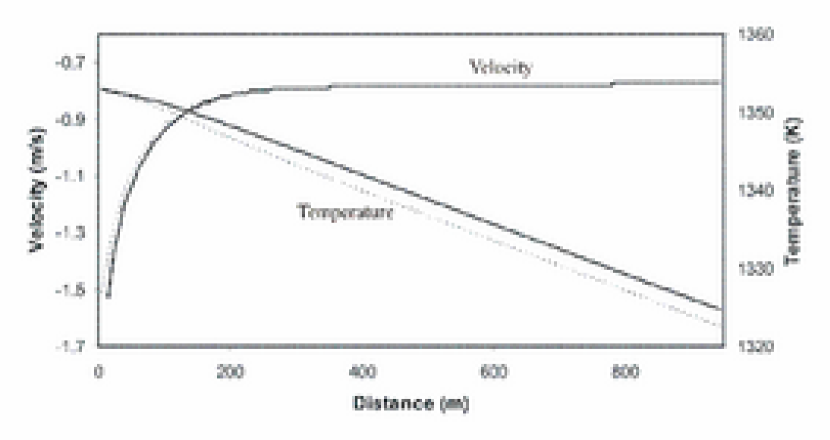
Figure 1: Longitudinal profiles of the channel center velocity and temperature, at $t=2500$ s. Dashed and continuous lines indicate analytical and numerical results, respectively. Channel dimensions: 50 m wide, 1000 m long; Slope: 0.1, $T_{env}=0$ K; $T_{0}=1353$ K, Flow rate: $Q=12.5$ m³/s; $\Delta x=\Delta y=5$ m.

Simulation results have shown a good agreement with an error less than 1% for the conservative variables $h$, $hV$ and $hT$ and, within a few % for the non-conservative variable $V$ and $T$. Moreover, in order to estimate the importance of each term on the right side of the equation (4), we considered the same geometry of the simple slope flow as above and the typical values reported in the caption of the Figure 2. Results, plotted in the Figure 2, show that radiative cooling is the main heat loss mechanism, while conductive and atmospheric convective cooling is less important but, for the parameter values used here, conductive loss is comparable with convection cooling. Viscous heating effect can be neglected in terms of mean lava temperature (in the simulated case it produces a increase of a few ^oC for a distance of 1 km), although, in certain conditions, it could be more important and determinant in the choosing the appropriate wall conditions and exchange coefficients for both momentum and energy (Costa and Macedonio, 2003).

Figure 2: Longitudinal temperature profiles at $t=2500$ s obtained using the same parameters of Figure 1 and $T_{env}=300$ K, $T_{c}=1173$ K, $f=0.5$, $\epsilon=0.8$, $n=4$, $m=12$. V.H. = Viscous Heating.

About effects of the coupling between momentum and energy equations, we can see a non-zero $b$ is important to determine the longitudinal variation of the lava flow thickness (see Figure 3), although it increases slightly the cooling beyond certain distances. Figure 3 shows as the velocity decrease due to the longitudinal viscosity increase is able to cause a longitudinal rise of the lava thickness because of the viscosity temperature dependence.

Figure 3: Longitudinal thickness profiles at $t=1200$ s obtained considering the same parameters reported in Figure 2.

4 Application to Etna lava flows

In this section, as an application, we reported simulation results of the initial phases of the 1991-1993 Etna eruption for which some field data for input and comparison are available (Calvari et al., 1994). In particular we simulated the second phase occurred from the $3^{rd}$ up to the $10^{th}$ January 1992. In order to estimate previously introduced semi-empirical parameters, we considered the typical magma parameters reported in Table 1 partially derived from data of Calvari et al. (1994). We assumed as representative an effective viscosity of 10³ Pa$\cdot$s at an estimated vent temperature of about 1353 K and $b\approx 0.02$ K^-1 that, for a cooling of about 100 K, reproduces the observed viscosities of the order of 10⁴ Pa$\cdot$s (Calvari et al., 1994). Other parameters were chosen within typical ranges: $f=0.1$ (between 0.01 and 1 (Keszthely and Self, 1998)), and $\epsilon=0.8$ (between 0.6 and 0.9 (Neri, 1998)). $T_{c}$ is set higher than its typical values since, for numerical reasons, we need to limit the maximum viscosity value.
The parameters reported in Table 1 give the following typical values:

$$\begin{array}[]{l}\displaystyle{\mathcal{H}}\sim 3/h\times 10^{-6}\,\mbox{m s}^{-1}\\ {\mathcal{E}}\approx 1.5\times 10^{-15}\,\mbox{m s}^{-1}\mbox{K}^{-3}\\ {\mathcal{W}}\approx 2\times 10^{-6}\,\mbox{m s}^{-1}\\ {\mathcal{K}}\sim 4/h\times 10^{-3}\,\mbox{m s}^{-1}\mbox{K}\\ \end{array}$$ (12)

where, for our aim in this application, we set $T_{env}=300$ K, $n=4$, $m=12$ and $\beta_{ij}=1$.

Table 1: Parameters characteristic of Etna lava.

$\rho$	2500	kg/m3
$b$	0.02	K-1
$c_{p}$	1200	J kg-1K-1
$k$	2.0	W m-1K-1
$\lambda$	70	Wm-2K-1
$T_{c}$	1253	K
$T_{0}$	1353	K
$\mu_{r}=\mu(T_{0})$	$10^{3}$	Pa s

As topographic basis, we used the digital data files of the Etna maps with a 1:10000 scale available at the Osservatorio Vesuviano-INGV web site at http://venus.ov.ingv.it (the used spatial grid resolution was $\Delta~{}x~{}=~{}\Delta~{}y~{}=~{}25$ m). For the second phase, we considered an ephemeral vent sited in Piano del Trifoglietto at the UTM coordinates (503795; 4174843). Finally, for the period 3-10 January 1992, we considered a constant average lava flow rate of 16 m³/s (ranging from 8 to 25 m³/s) (Calvari et al., 1994; Barberi et al., 1993).
The first phase of the eruption corresponded with the initial spreading of the lava flows on Piano del Trifoglietto. On the $3^{rd}$ January 1992 a new lava flow that overlapped the older lava lows, became an independent branch. By the evening it covered more than 1 km. The day after the front reached Mt. Calanna. One branch continued to move to the south of Mt. Calanna and one branch turned to the north then to the east (see Figure 3 of Calvari et al. (1994)). Because of a significantly decrease of lava supply, the southern lava flow stopped in Val Calanna. On January $7^{th}$ the northern lava lobe touched the southern one and then merged (Calvari et al., 1994).
In Figure 4 the simulated lava flow at the end of the second phase is shown. The model is able to reproduce semi-quantitatively the behaviour of the real lava flow and the order of magnitude of the quantities involved such as thickness, temperature and the time of front propagation of the lava flow. Although we introduced different simplifications and we considered an arduous case encompassing both a large viscous friction term and complex rough topography, the simulation and real lava flows show strikingly similar dynamics and thermal pattern evolution. Nevertheless the model presented in this paper remains an initial model of lava flow emplacement using SWE. Future improvements are expected by refining the the computational performance of the model and the formulation of the parameters.

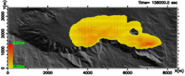
Figure 4: Simulated lava thickness of the $3^{rd}$ and $4^{th}$ January Etna lava flow.

5 Limitations

This methodology is based on vertical averages and therefore it cannot be rigorously valid for every conceivable application. We stress that the model is based on the basic assumptions of (1) small vertical scale relative to horizontal ($H_{*}^{2}/L_{*}^{2}\ll 1$), (2) homogeneous incompressible fluid, (3) hydrostatic pressure distribution, (4) slow vertical variations.
Concerning the computational method, the principal limit is related to the numerical treatment we used here for the source terms arising from topography and viscous friction. In particular since the actual topographies may contain abrupt variations, the slope term that appears in the equations (2) and (3) can become infinite in correspondence of discontinuities leading to numerical oscillations, diffusion, smearing and non-physical solutions (LeVeque, 1998; Alcrudo and Benkhaldoun, 2001; Chinnayya et al., 2004). Also the friction term must be carefully treated. In fact, if the characteristic time of the source term is much smaller than the characteristic time of the convective part of the equations, the problem is said to be stiff and the classical splitting method may provide erroneous physical solutions on coarse meshes (Chinnayya et al., 2004). To avoid these problems a trivial solution is using a very small time step, which results in long computational times. In the next version of the model, this limit could be overcome by applying directly a method based on the solution of the inhomogeneous Riemann problem with source term instead of applying the splitting method (Chinnayya et al., 2004; George, 2004).

6 Conclusion

A new general computational model for lava flow propagation based on the solution of depth-averaged equations for mass, momentum and energy equation was described. This approach appears to be a robust physical description and a good compromise between the full 3-D simulation and the necessity to decrease the computational time. The model was satisfactorily applied to reproduce some analytical solutions and to simulate a real lava flow event occurred during the 1991-93 Etna eruption. The good performance obtained in this preliminary version of the model makes this approach a potential tool to forecast reliably lava flow paths to use for risk mitigation, although the used algorithm should be improved for a better treatment of the source terms. This work was partially supported by the Gruppo Nazionale per la Vulcanologia-INGV and the Italian Department of the Civil Protection. This study was partially developed during the first author’s PhD at University of Bologna, Italy.

References

- Alcrudo and Benkhaldoun (2001) Alcrudo, F., and F. Benkhaldoun, Exact solutions to the Riemann of the shallow water equations with a step, Computers & Fluids, 30, 643–671, 2001.
- Ambrosi (1999) Ambrosi, D., Approximation of shallow water equations by Riemann solvers, Int. J. for Numer. Meth. in Fluids, 20, 157–168, 1999.
- Barberi et al. (1993) Barberi, F., M. Carapezza, M. Valenza, and L. Villari, The control of lava flow during the 1991-1992 eruption of Mt. Etna, J. Volcanol. Geotherm. Res., 56, 1–34, 1993.
- Burguete et al. (2002) Burguete, J., P. Garcia-Navarro, and R. Aliod, Numerical simulation of runoff from extreme rainfall events in a mountain water catchment, Nat. Haz. Earth Syst. Sci., 2, 109–117, 2002.
- Calvari et al. (1994) Calvari, S., M. Coltelli, M. Neri, M. Pompilio, and V. Scribano, The 1991-93 Etna eruption: chronology and flow-field evolution, Acta Vulcanol., pp. 1–15, 1994.
- Chinnayya et al. (2004) Chinnayya, A., A. LeRoux, and N. Seguin, A well-balanced numerical scheme for the approximation of the shallow-water equations with topography: the resonance phenomenon, International Journal on Finite Volumes, 2004.
- Costa and Macedonio (2002) Costa, A., and G. Macedonio, Nonlinear phenomena in fluids with temperature-dependent viscosity: an hysteresis model for magma flow in conduits, Geophys. Res. Lett., 29, 2002.
- Costa and Macedonio (2003) Costa, A., and G. Macedonio, Viscous heating in fluids with temperature-dependent viscosity: implications for magma flows, Nonlinear Proc. Geophys., 10, 545–555, 2003.
- Crisp and Baloga (1990) Crisp, J., and S. Baloga, A model for lava flows with two thermal components, J. Geophys. Res., 95, 1255–1270, 1990.
- Ferrari and Saleri (2004) Ferrari, S., and F. Saleri, A new two-dimensional shallow water model including pressure effects and slow varying bottom topography, ESAIM: Mathematical Modelling and Numerical Analisys, 38, 211–234, 2004.
- George (2004) George, D., Numerical Approximation of the Nonlinear Shallow Water Equations with Topography and Dry Beds: A Godunov-Type Scheme, Master’s thesis, University of Washington, 2004.
- Gerbeau and Perthame (2001) Gerbeau, J., and B. Perthame, Derivation of viscous Saint-Venant system for laminar shallow water; numerical validation, Discret. Contin. Dyn.-B, 1, 89–102, 2001.
- Heinrich et al. (2001) Heinrich, P., A. Piatanesi, and H. Hébert, Numerical modelling of tsunami generation and propagation from submarine slumps: the 1998 Papua New Guinea event, Geophys. J. Int., 145, 97–111, 2001.
- Keszthely and Self (1998) Keszthely, L., and S. Self, Some physical requirements for the emplacement of long basaltic lava flows, J. Geophys. Res., 103, 27,447–27,464, 1998.
- LeVeque (1998) LeVeque, R., Balancing source terms and flux gradients in high-resolution Godunov methods: the quasi-steady wave-propagation algorithm, J. Comput. Phys., 146, 346–365, 1998.
- LeVeque (2002) LeVeque, R., Finite Volume Methods for Hyperbolic Problems, Cambridge University Press, 2002.
- Monthe et al. (1999) Monthe, L., F. Benkhaldoun, and I. Elmahi, Positivity preserving finite volume Roe schemes for transport-diffusion equations, Comput. Methods Appl. Mech. Engrg., 178, 215–232, 1999.
- Neri (1998) Neri, A., A local heat transfer analysis of lava cooling in the atmosphere: application to thermal diffusion-dominated lava flows, J. Volcanol. Geotherm. Res., 81, 215–243, 1998.
- Pieri and Baloga (1986) Pieri, D., and S. Baloga, Eruption rate, area, and length relationships for some Hawaiian lava flows, J. Volcanol. Geotherm. Res., 30, 29–45, 1986.
- Shah and Pearson (1974) Shah, Y., and J. Pearson, Stability of non-isothermal flow in channels - III. Temperature-dependent pawer-law fluids with heat generation, Chem. Engng. Sci., 29, 1485–1493, 1974.